Numerical Study of the Pyrolysis of Wood Chips for Biocharcoal Production: Influence of Chips Geometry and Initial Moisture Content

Abstract

This study presents the modeling of wood chips pyrolysis, considering the initial moisture content and taking into account the near-parallelepiped geometry of common wood chips, which is not available among the simulated shapes of wood in the literature. The goal is to extend the research and generate useful data on how different varieties of shapes and initial moisture contents influence wood chips pyrolysis. The effects of temperature and thickness variation on the pressure of volatile products, core temperature, and densities of pyrolysis products were studied. The model was validated with the mass fraction of experimental data obtained from beechwood chips with a density of 700 kg/m³ and thickness of 10 mm–30 mm at 973.15 K–1273.15 K. The mean absolute error (MAE) and mean relative error (MRE) values were, respectively, 0.066 and 10.376% at 973.15 K, and 0.065 and 22.632% at 1273.15 K. High temperature favored the rate of biocharcoal production from the surface to the core, though part of the biocharcoal was lost at the surface.

1. Introduction

Wood products are used in building, packaging, furnishing, energy generation, and more [1]. Wood is constituted of three main chemical components: cellulose, hemicelluloses, and lignin. Some studies show that wood composition depends on the origin, maturity, and species type [2,3,4]. The composition of wood is also influenced by the type of wood (hardwood, softwood, pine back, husks, peat, etc.) [5]. During the production of wood products, a lot of biomass is produced in the form of wood chips, sawdust, ash, and so on. Wood, as lignocellulosic biomass, is efficient in the production of clean, renewable, and sustainable fuels [6,7]. This can be achieved by applying different energy-harnessing methods. The most common method applied is the controlled thermal decomposition of the biomass at different temperature ranges to yield biogas, bio-oil, and biocharcoal for different applications [8,9]. The technologies available to do this include combustion, gasification, and pyrolysis processes. However, pyrolysis is the only process capable of collectively producing condensable gas, liquid fuel, and charcoal at a temperature ranging between 400 and 600 °C [9,10]. Pyrolysis has been proven to be an efficient conversion process for producing alternative fuel and biocharcoal with low greenhouse gas emissions [11]. Among the byproducts of pyrolysis, biocharcoal can be easily utilized in most African countries for agricultural purposes, since the technology to refine the gas and liquid oil as energy is lacking. Applications of biocharcoal in the co-firing of plants and metallurgical processes have also been reported [12,13].

In most cases, the challenge in adopting the pyrolysis method to generate energy and biocharcoal is the cost of building the plant, which first requires the study of operating parameters [14]. These parameters are usually generated through costly experimental studies. The setback is that the data required for optimization purposes are limited in the literature for different biomass compositions. Nevertheless, the advent of different computational software has presented powerful tools to numerically simulate all operational conditions, which can be brought to reality in physical designs of pyrolysis [15]. Several numerical simulation studies for biomass including wood chips are available in the literature [16,17]. Successful modeling of the process depends on knowledge of the reaction scheme, which is a complex process. This reaction scheme depends on the mechanism of the heat and mass transfer between the reactor and the product. The dynamics of heat flux surrounding the wood chips, as heat is transferred from the surface to the core, are related to their shape [18,19]. Investigating some possible shapes of wood chips, the authors of [18,19] showed that the pyrolysis duration and the final mass fraction are shape dependent. The intra-particle structural dynamics of the wood chips are also affected by the shapes. The shape of the biomass during pyrolysis can lead to differences in the characteristic length of the transport phenomenon for heat and mass transfer [20]. However, the authors of [18] simplified their choice of shapes for ease of numerical simulations. Considering the effect of the shape of wood chips on heat and mass transport phenomenon and product yield, Atreya et al. [19] studied cuboids, cylinders, and spherical shapes. They found that the duration for completion of the pyrolysis processes, mass loss measurement, iso-surface for internal pressure, and heat generation was highest for spheres and lowest for cubic shapes, and that these measures are affected by the shortest distance for heat and mass transfer. Okekunle et al. [18] considered cylindrical, rectangular, equant, and disc-shaped wood chips in their pyrolysis studies. They observed high biochar yield for rectangular shapes at a lower temperature. Park et al. [21] considered spherical shapes and observed sample splitting due to the weakness of the structure and the generation of internal pressure. However, they suggested that moisture content, which they did not study, might have the same effects as the internal pressure and structural weakness on the wood chips during pyrolysis. Although these simplified shapes of wood chips have been studied for ease of numerical simulations, a closer observation of wood chips can present diverse shapes. In Africa and some developing countries, wood processing is still dominated by traditional semi-automatic and economical wood saw methods. As a result, it suffers from positioning errors, which include non-central alignment of saw pattern and non-parallel direction of the infeed, thus commonly producing near-parallelepiped-shaped chips [22], as shown in Figure 1.

A thorough search of the literature showed that no study has adopted a near-parallelepiped shape in the numerical simulation of wood chips pyrolysis to study the heat and mass transport phenomena. This is important, as this shape might be the predominant shape of wood chips generated in Africa and other countries, and it can be central to the optimum design of pyrolysis plants in Africa. Therefore, this work aimed to extend the study of Park et al. [21] and Atreya et al. [19] to include parallelepiped-shaped chips, with more emphasis on producing more biocharcoal. This will include the influence of initial moisture content omitted by Park et al. [21], because of its importance in modifying the thermo-physical properties of the wood [24,25,26,27].

2. Model Developments

The multi-reaction approach proposed by Di-Blasi and Russo [28] was used in this study (Figure 2a). Two scenarios were followed in the simulation process. In the first case, the wood is considered dry (Figure 2a), while in the second case (Figure 2b), the wood is considered not dry but humid, and it has a high initial moisture content. The second case is taken to integrate the suggestion of Park et al. [21]. Vapor is considered to be generated during the primary reactions. During these reactions, gas, tar, and charcoal are produced. The secondary reactions allow for the transformation of a part of the produced tar into gas and biocharcoal.

In the first case, because the wood is considered completely dry, the drying process is neglected, and the heat balance and mass conservation equations for solids, gases, steam, and liquid are written as follows [21,28,29,30]:

$$\{\begin{array}{c}\left({\mathsf{\rho }}_{\mathrm{b}}{\mathrm{C}}_{\mathrm{pb}}+{\mathsf{\rho }}_{\mathrm{c}}{\mathrm{C}}_{\mathrm{pc}}+{ϵ}_{\mathrm{por}}\left({\mathsf{\rho }}_{\mathrm{g}}{\mathrm{C}}_{\mathrm{pg}}+{\mathsf{\rho }}_{\mathrm{t}}{\mathrm{C}}_{\mathrm{pt}}\right)\right)\frac{\partial \mathrm{T}}{\partial \mathrm{t}}=-\left({\mathsf{\rho }}_{\mathrm{g}}{\mathrm{C}}_{\mathrm{pg}}+{\mathsf{\rho }}_{\mathrm{t}}{\mathrm{C}}_{\mathrm{pt}}\right)\mathrm{u}\frac{\partial \mathrm{T}}{\partial \mathrm{x}}+\mathsf{\lambda }\frac{{\partial }^2\mathrm{T}}{\partial {\mathrm{x}}^2}+{\mathrm{Q}}_{\mathrm{r}}^{″}\\ \frac{\partial {\mathsf{\rho }}_{\mathrm{b}}}{\partial \mathrm{t}}=-\left({\mathrm{k}}_{\mathrm{c}}+{\mathrm{k}}_{\mathrm{g}}+{\mathrm{k}}_{\mathrm{t}}\right){\mathsf{\rho }}_{\mathrm{b}}\\ \frac{\partial {\mathsf{\rho }}_{\mathrm{c}}}{\partial \mathrm{t}}={\mathrm{k}}_{\mathrm{c}}{\mathsf{\rho }}_{\mathrm{b}}+{ϵ}_{\mathrm{por}}{\mathrm{k}}_{\mathrm{c}2}{\mathsf{\rho }}_{\mathrm{t}}\\ \frac{\partial \left({ϵ}_{\mathrm{por}}{\mathsf{\rho }}_{\mathrm{g}}\right)}{\partial \mathrm{t}}+\frac{\partial \left({\mathsf{\rho }}_{\mathrm{g}}\mathrm{u}\right)}{\partial \mathrm{x}}={\mathrm{k}}_{\mathrm{g}}{\mathsf{\rho }}_{\mathrm{b}}+{ϵ}_{\mathrm{por}}{\mathrm{k}}_{\mathrm{g}2}{\mathsf{\rho }}_{\mathrm{t}}\\ \frac{\partial \left({ϵ}_{\mathrm{por}}{\mathsf{\rho }}_{\mathrm{t}}\right)}{\partial \mathrm{t}}+\frac{\partial \left({\mathsf{\rho }}_{\mathrm{t}}\mathrm{u}\right)}{\partial \mathrm{x}}={\mathrm{k}}_{\mathrm{t}}{\mathsf{\rho }}_{\mathrm{b}}-{ϵ}_{\mathrm{por}}\left({\mathrm{k}}_{\mathrm{c}2}+{\mathrm{k}}_{\mathrm{g}2}\right){\mathsf{\rho }}_{\mathrm{t}}\end{array}$$

(1)

$${\mathrm{Q}}_{\mathrm{r}}^{″}={\mathrm{Q}}_{\mathrm{end}}^{″}+{\mathrm{Q}}_{\mathrm{exo}}^{″}$$

(2)

$${\mathrm{Q}}_{\mathrm{end}}^{″}={\mathsf{\rho }}_{\mathrm{b}}\left({\mathrm{k}}_{\mathrm{g}}{\mathsf{\Delta }\mathrm{h}}_{\mathrm{g}}+{\mathrm{k}}_{\mathrm{t}}{\mathsf{\Delta }\mathrm{h}}_{\mathrm{t}}+{\mathrm{k}}_{\mathrm{c}}{\mathsf{\Delta }\mathrm{h}}_{\mathrm{c}}\right);{\mathrm{Q}}_{\mathrm{exo}}^{″}={ϵ}_{\mathrm{por}}{\mathsf{\rho }}_{\mathrm{t}}\left({\mathrm{k}}_{\mathrm{g}2}{\mathsf{\Delta }\mathrm{h}}_{\mathrm{g}2}+{\mathrm{k}}_{\mathrm{c}2}{\mathsf{\Delta }\mathrm{h}}_{\mathrm{c}2}\right)$$

(3)

Parameters k_i are given in

Table 1. Constants used [28,29].

Parameters	${\mathbf{E}}_{\mathbf{i}} \left(\mathbf{J}/\mathbf{m}\mathbf{o}\mathbf{l}\right)$	${\mathbf{A}}_{\mathbf{i}}$$\left({\mathbf{s}}^{-1}\right)$
${\mathrm{k}}_1$(${\mathrm{s}}^{-1}$)	$88.6\times {10}^3$	$5.16\times {10}^6$
${\mathrm{k}}_2$(${\mathrm{s}}^{-1}$)	$112.7\times {10}^3$	$1.48\times {10}^{10}$
${\mathrm{k}}_3$(${\mathrm{s}}^{-1}$)	$106.5\times {10}^3$	$2.66\times {10}^{10}$
${\mathrm{k}}_{\mathrm{g}2}$(${\mathrm{s}}^{-1}$)	$108\times {10}^3$	$4.28\times {10}^6$
${\mathrm{k}}_{\mathrm{c}2}$(${\mathrm{s}}^{-1}$)	$108\times {10}^3$	$1.00\times {10}^6$

. To add the influence of vapor for the second case, where the wood is not dry, the heat transfer (first equation of the set 1) is modified as follows:

$$\left({\mathsf{\rho }}_{\mathrm{b}}{\mathrm{C}}_{\mathrm{pb}}+{\mathsf{\rho }}_{\mathrm{c}}{\mathrm{C}}_{\mathrm{pc}}+{ϵ}_{\mathrm{por}}\left({\mathsf{\rho }}_{\mathrm{g}}{\mathrm{C}}_{\mathrm{pg}}+{\mathsf{\rho }}_{\mathrm{t}}{\mathrm{C}}_{\mathrm{pt}}\right)\right)\frac{\partial \mathrm{T}}{\partial \mathrm{t}}=-\left({\mathsf{\rho }}_{\mathrm{g}}{\mathrm{C}}_{\mathrm{pg}}+{\mathsf{\rho }}_{\mathrm{t}}{\mathrm{C}}_{\mathrm{pt}}\right)\mathrm{u}\frac{\partial \mathrm{T}}{\partial \mathrm{x}}+\mathsf{\lambda }\frac{{\partial }^2\mathrm{T}}{\partial {\mathrm{x}}^2}+{\mathrm{Q}}_{\mathrm{r}}^{″}-{\mathrm{k}}_{\mathrm{v}}{\mathsf{\rho }}_{\mathrm{m}}{ϵ}_{\mathrm{por}}{\mathrm{HL}}_{\mathrm{v}}$$

(4)

Mass transfer of vapor is given by:

$$\frac{\partial \mathrm{H}}{\partial \mathrm{t}}={\mathrm{D}}_{\mathrm{H}}\left(\frac{{\partial }^2\mathrm{H}}{\partial {\mathrm{x}}^2}\right)$$

(5)

The boundary equation of humidity is given by:

$${\mathrm{D}}_{\mathrm{H}}\frac{\partial \mathrm{H}}{\partial \mathrm{x}}\overrightarrow{\mathrm{n}}={\mathrm{h}}_{\mathrm{m}}\left({\mathrm{X}}_{\mathrm{eq}}-\mathrm{H}\right){\overrightarrow{\mathrm{n}}}_1$$

(6)

To consider the presence of water in wood, the equilibrium moisture content, X_eq, is calculated according to the relation of Simpson and TenWolde [31]:

$${\mathrm{X}}_{\mathrm{eq}}=\frac{18}{\mathrm{A}}\left(\frac{\mathrm{B}\times \mathrm{RH}}{1-\mathrm{B}\times \mathrm{RH}}+\frac{\mathrm{C}\times \mathrm{B}\times \mathrm{RH}+2\times \mathrm{C}\times \mathrm{D}\times {\mathrm{B}}^2\times {\mathrm{RH}}^2}{1+\mathrm{C}\times \mathrm{B}\times \mathrm{RH}+\mathrm{C}\times \mathrm{D}\times {\mathrm{B}}^2\times {\mathrm{RH}}^2}\right)$$

(7)

Coefficients A, B, C, and D are given in

Table 2. Material properties and kinetic parameters for model equations.

Parameters	Values	References
${\rho }_g$	${\mathsf{\rho }}_{\mathrm{G}}+{\mathsf{\rho }}_{\mathrm{t}}$	[16]
${ϵ}_{por}$	$1-\frac{{\mathsf{\rho }}_{\mathrm{b}}}{1500}$	[24]
$\lambda$	${\mathsf{\eta }\mathsf{\lambda }}_{\mathrm{b}}+\left(1-\mathsf{\eta }\right){\mathsf{\lambda }}_{\mathrm{c}}+{ϵ}_{\mathrm{por}}{\mathsf{\lambda }}_{\mathrm{g}}+{\mathsf{\sigma }\mathrm{T}}^3\mathrm{d}/\mathsf{\epsilon }$	[16]
d	$4\times {10}^{-5}\mathrm{m}$ a	[16]
$\epsilon$	$1$	[16]
${\lambda }_b$	$0.1046\mathrm{W}/\left(\mathrm{m}.\mathrm{K}\right)$	[32]
${\lambda }_c$	$0.071\mathrm{W}/\left(\mathrm{m}.\mathrm{K}\right)$	[32]
${\lambda }_g$	$0.025\mathrm{W}/\left(\mathrm{m}.\mathrm{K}\right)$	[32]
$\sigma$	$5.67\times {10}^{-8}\mathrm{J}{\mathrm{s}}^{-1}{\mathrm{m}}^{-2}{\mathrm{K}}^{-4}$	[24]
$\eta$	${\mathsf{\rho }}_{\mathrm{b}}/{\mathsf{\rho }}_{\mathrm{b}0}$	[16]
$\Delta h_g; \Delta h_t;\Delta h_c$	$-418\times {10}^3\mathrm{J}/\mathrm{kg}$	[16]
$\Delta h_{g\mathbf{2}}; \Delta h_{c\mathbf{2}}$	$42\times {10}^3\mathrm{J}/\mathrm{kg}$	[16]
$C_{pb}$	$1400+0.3\mathrm{T}$	[32]
$C_{pc}$	$\left(0.42+0.09\times {10}^{-3}\mathrm{T}+6.85\times {10}^{-7}{\mathrm{T}}^2\right)\times {10}^3$	[32]
$C_{pt}$	$\left(-0.1+4.4\times {10}^{-3}\mathrm{T}-1.57\times {10}^{-6}{\mathrm{T}}^2\right)\times {10}^3$	[32]
$C_{pg}$	$\left(0.77+6.29\times {10}^{-4}\mathrm{T}-1.91\times {10}^{-7}{\mathrm{T}}^2\right)\times {10}^3$	[32]
$K_b$	$1.18\times {10}^{-19}{\mathrm{m}}^2$ (tangential)	[32]
$K_c$	$1.28\times {10}^{-18}{\mathrm{m}}^2$ (radial)	[32]
$\mu$	$8.5\times {10}^{-6}+0.0296\times {10}^{-6}\mathrm{T}\left(\mathrm{kg}/\left(\mathrm{m}.\mathrm{s}\right)\right)$	[32]
$M_g$	$75\times {10}^{-3}\mathrm{kg}/\mathrm{mol}$	[32]
$k_v$	${\mathrm{A}}_{{\mathrm{H}}_2\mathrm{O}}{\mathrm{T}}^{\frac{-1}{2}}\exp \left(-\frac{{\mathrm{E}}_{{\mathrm{H}}_2\mathrm{O}}}{\mathrm{R}.\mathrm{T}}\right)$	[4,24,25,26,27,33,34,35,36,37]
$A_{H_{\mathbf{2}}O}$	$6\times {10}^5{\mathrm{s}}^{-1}{\mathrm{K}}^{1/2}$	[4,24,25,26,27,33,34,35,36,37]
$E_{H_{\mathbf{2}}O}$	$48.22\times {10}^3\mathrm{J}.{\mathrm{mol}}^{-1}$	[4,24,25,26,27,33,34,35,36,37]
$A$	$349+1.29{\mathrm{T}}_{\mathrm{a}}+0.0135{\mathrm{T}}_{\mathrm{a}}{}^2$	[24]
$B$	$0.805+0.000736{\mathrm{T}}_{\mathrm{a}}-0.00000273{\mathrm{T}}_{\mathrm{a}}{}^2$	[24]
$C$	$6.27-0.00938{\mathrm{T}}_{\mathrm{a}}-0.000303{\mathrm{T}}_{\mathrm{a}}{}^2$	[24]
$D$	$1.93+0.0407{\mathrm{T}}_{\mathrm{a}}-0.000293{\mathrm{T}}_{\mathrm{a}}{}^2$	[24]
$D_H$	$\exp \left(-9.9+9.8{\mathrm{X}}_{\mathrm{eq}}-\frac{4300}{{\mathrm{T}}_{\mathrm{a}}}\right)$	[24]
Lv	(3335$-$2.91 T) × 103 (J/kg)	[24]
${\lambda }_b$	$\frac{{\mathsf{\rho }}_{\mathrm{b}}}{{\mathsf{\rho }}_{\mathrm{l}}}\left(0.2003+0.00548\mathrm{H}\right)+0.02378$ (W/(m.K)	[24]
$C_{pb}$	$\frac{{\mathrm{C}}_{\mathrm{po}}+{\mathrm{HC}}_{\mathrm{pw}}}{1+\mathrm{H}}+\mathrm{H}\left(-0.06191+2.36\times {10}^{-4}\mathrm{T}-1.33\times {10}^{-4}\mathrm{H}\right)$ (kJ/(kg. K)	[24]
$C_{po}$	$0.1031+0.003867\mathrm{T}$ (kJ/(kg. K)	[24]
$C_{pw}$	4.19 (kJ/(kg. K)	[24]

, with T in °C. RH is the relative humidity of air in %/100. To add the influence of moisture in the second case, the mass conservation Equation (1) in the first case for gas is modified to add water vapor as follows:

$$\{\begin{array}{c}\frac{\partial {\mathsf{\rho }}_{\mathrm{v}}}{\partial \mathrm{t}}={\mathrm{k}}_{\mathrm{v}}{\mathsf{\rho }}_{\mathrm{b}}\\ \frac{\partial {\mathsf{\rho }}_{\mathrm{b}}}{\partial \mathrm{t}}=-\left({\mathrm{k}}_{\mathrm{v}}+{\mathrm{k}}_{\mathrm{c}}+{\mathrm{k}}_{\mathrm{g}}+{\mathrm{k}}_{\mathrm{t}}\right){\mathsf{\rho }}_{\mathrm{b}}\end{array}$$

(8)

Initial values and boundary equations are described below.

Initial conditions are as follows:

$\mathrm{T}={\mathrm{T}}_{\mathrm{o}}=293.15\mathrm{K}$, ${\mathsf{\rho }}_{\mathrm{b}}={\mathsf{\rho }}_{{\mathrm{b}}_{\mathrm{o}}}=700\mathrm{kg}/{\mathrm{m}}^3$, ${\mathsf{\rho }}_{\mathrm{c}}={\mathsf{\rho }}_{\mathrm{t}}={\mathsf{\rho }}_{\mathrm{g}}=0\mathrm{kg}/{\mathrm{m}}^3$, $\mathrm{u}=0$.

The boundary equation of heat transfer is given by:

$$\mathsf{\lambda }\frac{\partial \mathrm{T}}{\partial \mathrm{x}}\overrightarrow{\mathrm{n}}=\left({\mathrm{q}}_{\mathrm{i}}+\mathsf{\sigma }\left({{\mathrm{T}}_{\mathrm{fi}}}^4-{{\mathrm{T}}_{\mathrm{i}=0,\max }}^4\right)+{\mathrm{h}}_{\mathrm{conv}}{}_{\mathrm{i}}\left({\mathrm{T}}_{\mathrm{a}}{}_{\mathrm{i}}-{\mathrm{T}}_{\mathrm{i}=0,\max }\right)\right){\overrightarrow{\mathrm{n}}}_1$$

(9)

The intensity of the radiative heat flux qi was taken as 0 kW.m⁻²–45 kW.m⁻², depending on the situation. Parameters, such as activation energies and frequency constant, are given by Di-Blasi and Russo [28] and Gronli [29] and are presented in Table 1.

Pressure Evolution

Assuming a perfect gas, the pressure evolution equation gives:

$$\frac{\partial }{\partial \mathrm{t}}\left(\frac{{ϵ}_{\mathrm{por}}\mathrm{P}}{\mathrm{T}}\right)=\frac{1}{2}\frac{\partial }{\partial \mathrm{x}}\left(\frac{\mathrm{K}}{\mathsf{\mu }\mathrm{T}}\frac{\partial {\mathrm{P}}^2}{\partial \mathrm{x}}\right)+\frac{{\mathrm{Rw}}_{\mathrm{g}}}{{\mathrm{M}}_{\mathrm{g}}}$$

(10)

$${\mathrm{W}}_{\mathrm{g}}=\frac{\partial \left[{ϵ}_{\mathrm{por}}\left({\mathsf{\rho }}_{\mathrm{G}}+{\mathsf{\rho }}_{\mathrm{t}}\right)\right]}{\partial \mathrm{t}}+\frac{\partial \left[\mathrm{u}\left({\mathsf{\rho }}_{\mathrm{g}}+{\mathsf{\rho }}_{\mathrm{t}}\right)\right]}{\partial \mathrm{x}}$$

(11)

The perfect gases constant is given by R = 8.314 J/(mol.K). Using Darcy’s law, the velocity of total gases (tar + gas) can be estimated. Thus, we have:

$$\mathrm{u}=-\frac{\mathrm{K}}{\mathsf{\mu }}\frac{\partial \mathrm{P}}{\partial \mathrm{x}}$$

(12)

Intrinsic permeabilities (K) of wood have been taken from Gronli [29] and are given by:

$$\mathrm{K}={\mathsf{\eta }\mathrm{K}}_{\mathrm{b}}+\left(1-\mathsf{\eta }\right){\mathrm{K}}_{\mathrm{c}}$$

(13)

The material properties and kinetic parameters for all the model equations are presented in Table 2 below.

Numerical Simulation Procedure

The numerical equations were solved using the finite differences method in Fortran 90, and the iteration time steps is 0.05 s, and each sample divided in 61 parts. To incorporate the geometry of the shape in the simulation, the i and j nodes indicating space and time were used to obtain convergency of the simulated results. The simulation algorithm is shown in Figure 3.

Heat transfer is given by:

$${\mathrm{T}}_{\mathrm{i}}^{\mathrm{j}+1}={\mathrm{A}}_{\mathrm{i}}^{\mathrm{j}}{\mathrm{T}}_{\mathrm{i}}^{\mathrm{j}}+{\mathrm{B}}_{\mathrm{i}}^{\mathrm{j}}{\mathrm{T}}_{\mathrm{i}+1}^{\mathrm{j}}+{\mathrm{C}}_{\mathrm{i}}^{\mathrm{j}}{\mathrm{T}}_{\mathrm{i}-1}^{\mathrm{j}}+{\mathrm{D}}_{\mathrm{i}}^{\mathrm{j}}$$

(14)

$${\mathrm{A}}_{\mathrm{i}}^{\mathrm{j}}=1+\frac{\left[\left({\mathsf{\rho }}_{\mathrm{g}}{}_{\mathrm{i}}^{\mathrm{j}}{\mathrm{C}}_{\mathrm{pg}}{}_{\mathrm{i}}^{\mathrm{j}}+{\mathsf{\rho }}_{\mathrm{t}}{}_{\mathrm{i}}^{\mathrm{j}}{\mathrm{C}}_{\mathrm{pt}}{}_{\mathrm{i}}^{\mathrm{j}}\right){\mathrm{u}}_{\mathrm{i}}^{\mathrm{j}}-\frac{2{\mathsf{\lambda }}_{\mathrm{i}}^{\mathrm{j}}}{\mathsf{\Delta }\mathrm{x}}\right]\mathsf{\Delta }\mathrm{t}}{\mathsf{\Delta }\mathrm{x}\left({\mathsf{\rho }}_{\mathrm{b}}{}_{\mathrm{i}}^{\mathrm{j}}{\mathrm{C}}_{\mathrm{pb}}{}_{\mathrm{i}}^{\mathrm{j}}+{\mathsf{\rho }}_{\mathrm{c}}{}_{\mathrm{i}}^{\mathrm{j}}{\mathrm{C}}_{\mathrm{pc}}{}_{\mathrm{i}}^{\mathrm{j}}+{ϵ}_{\mathrm{por}}{}_{\mathrm{i}}^{\mathrm{j}}\left({\mathsf{\rho }}_{\mathrm{g}}{}_{\mathrm{i}}^{\mathrm{j}}{\mathrm{C}}_{\mathrm{pg}}{}_{\mathrm{i}}^{\mathrm{j}}+{\mathsf{\rho }}_{\mathrm{t}}{}_{\mathrm{i}}^{\mathrm{j}}{\mathrm{C}}_{\mathrm{pt}}{}_{\mathrm{i}}^{\mathrm{j}}\right)\right)}$$

(15)

$${\mathrm{B}}_{\mathrm{i}}^{\mathrm{j}}=\frac{\left[\frac{{\mathsf{\lambda }}_{\mathrm{i}}^{\mathrm{j}}}{\mathsf{\Delta }\mathrm{x}}-\left({\mathsf{\rho }}_{\mathrm{g}}{}_{\mathrm{i}}^{\mathrm{j}}{\mathrm{C}}_{\mathrm{pg}}{}_{\mathrm{i}}^{\mathrm{j}}+{\mathsf{\rho }}_{\mathrm{t}}{}_{\mathrm{i}}^{\mathrm{j}}{\mathrm{C}}_{\mathrm{pt}}{}_{\mathrm{i}}^{\mathrm{j}}\right){\mathrm{u}}_{\mathrm{i}}^{\mathrm{j}}\right]\mathsf{\Delta }\mathrm{t}}{\mathsf{\Delta }\mathrm{x}\left({\mathsf{\rho }}_{\mathrm{b}}{}_{\mathrm{i}}^{\mathrm{j}}{\mathrm{C}}_{\mathrm{pb}}{}_{\mathrm{i}}^{\mathrm{j}}+{\mathsf{\rho }}_{\mathrm{c}}{}_{\mathrm{i}}^{\mathrm{j}}{\mathrm{C}}_{\mathrm{pc}}{}_{\mathrm{i}}^{\mathrm{j}}+{ϵ}_{\mathrm{por}}{}_{\mathrm{i}}^{\mathrm{j}}\left({\mathsf{\rho }}_{\mathrm{g}}{}_{\mathrm{i}}^{\mathrm{j}}{\mathrm{C}}_{\mathrm{pg}}{}_{\mathrm{i}}^{\mathrm{j}}+{\mathsf{\rho }}_{\mathrm{t}}{}_{\mathrm{i}}^{\mathrm{j}}{\mathrm{C}}_{\mathrm{pt}}{}_{\mathrm{i}}^{\mathrm{j}}\right)\right)}$$

(16)

$${\mathrm{C}}_{\mathrm{i}}^{\mathrm{j}}=\frac{{\mathsf{\lambda }}_{\mathrm{i}}^{\mathrm{j}}\Delta \mathrm{t}}{\left({\mathsf{\rho }}_{\mathrm{b}}{}_{\mathrm{i}}^{\mathrm{j}}{\mathrm{C}}_{\mathrm{pb}}{}_{\mathrm{i}}^{\mathrm{j}}+{\mathsf{\rho }}_{\mathrm{c}}{}_{\mathrm{i}}^{\mathrm{j}}{\mathrm{C}}_{\mathrm{pc}}{}_{\mathrm{i}}^{\mathrm{j}}+{ϵ}_{\mathrm{por}}{}_{\mathrm{i}}^{\mathrm{j}}\left({\mathsf{\rho }}_{\mathrm{g}}{}_{\mathrm{i}}^{\mathrm{j}}{\mathrm{C}}_{\mathrm{pg}}{}_{\mathrm{i}}^{\mathrm{j}}+{\mathsf{\rho }}_{\mathrm{t}}{}_{\mathrm{i}}^{\mathrm{j}}{\mathrm{C}}_{\mathrm{pt}}{}_{\mathrm{i}}^{\mathrm{j}}\right)\right){\left(\Delta \mathrm{x}\right)}^2}$$

(17)

$${\mathrm{D}}_{\mathrm{i}}^{\mathrm{j}}=\frac{{\mathrm{Q}}_{\mathrm{r}}^{″}{}_{\mathrm{i}}^{\mathrm{j}}\Delta \mathrm{t}}{\left({\mathsf{\rho }}_{\mathrm{b}}{}_{\mathrm{i}}^{\mathrm{j}}{\mathrm{C}}_{\mathrm{pb}}{}_{\mathrm{i}}^{\mathrm{j}}+{\mathsf{\rho }}_{\mathrm{c}}{}_{\mathrm{i}}^{\mathrm{j}}{\mathrm{C}}_{\mathrm{pc}}{}_{\mathrm{i}}^{\mathrm{j}}+{ϵ}_{\mathrm{por}}{}_{\mathrm{i}}^{\mathrm{j}}\left({\mathsf{\rho }}_{\mathrm{g}}{}_{\mathrm{i}}^{\mathrm{j}}{\mathrm{C}}_{\mathrm{pg}}{}_{\mathrm{i}}^{\mathrm{j}}+{\mathsf{\rho }}_{\mathrm{t}}{}_{\mathrm{i}}^{\mathrm{j}}{\mathrm{C}}_{\mathrm{pt}}{}_{\mathrm{i}}^{\mathrm{j}}\right)\right)}$$

(18)

When moisture content is considered, only ${\mathrm{D}}_{\mathrm{i}}^{\mathrm{j}}$ is changed to give:

$${\mathrm{D}}_{\mathrm{i}}^{\mathrm{j}}=\frac{\left({\mathrm{Q}}_{\mathrm{r}}^{″}{}_{\mathrm{i}}^{\mathrm{j}}-{\mathrm{k}}_{\mathrm{v}}{}_{\mathrm{i}}^{\mathrm{j}}{\mathsf{\rho }}_{\mathrm{m}}{}_{\mathrm{i}}^{\mathrm{j}}{\mathrm{L}}_{\mathrm{v}}{}_{\mathrm{i}}^{\mathrm{j}}\right)\Delta \mathrm{t}}{\left({\mathsf{\rho }}_{\mathrm{b}}{}_{\mathrm{i}}^{\mathrm{j}}{\mathrm{C}}_{\mathrm{pb}}{}_{\mathrm{i}}^{\mathrm{j}}+{\mathsf{\rho }}_{\mathrm{c}}{}_{\mathrm{i}}^{\mathrm{j}}{\mathrm{C}}_{\mathrm{pc}}{}_{\mathrm{i}}^{\mathrm{j}}+{ϵ}_{\mathrm{por}}{}_{\mathrm{i}}^{\mathrm{j}}\left({\mathsf{\rho }}_{\mathrm{g}}{}_{\mathrm{i}}^{\mathrm{j}}{\mathrm{C}}_{\mathrm{pg}}{}_{\mathrm{i}}^{\mathrm{j}}+{\mathsf{\rho }}_{\mathrm{t}}{}_{\mathrm{i}}^{\mathrm{j}}{\mathrm{C}}_{\mathrm{pt}}{}_{\mathrm{i}}^{\mathrm{j}}\right)\right)}$$

(19)

Mass transfer is given by:

$$\{\begin{array}{c}{\mathsf{\rho }}_{\mathrm{b}}{}_{\mathrm{i}}^{\mathrm{j}+1}=\left[1-\left({\mathrm{k}}_{\mathrm{c}}{}_{\mathrm{i}}^{\mathrm{j}}+{\mathrm{k}}_{\mathrm{g}}{}_{\mathrm{i}}^{\mathrm{j}}+{\mathrm{k}}_{\mathrm{t}}{}_{\mathrm{i}}^{\mathrm{j}}\right)\Delta \mathrm{t}\right]{\mathsf{\rho }}_{\mathrm{b}}{}_{\mathrm{i}}^{\mathrm{j}}\\ {\mathsf{\rho }}_{\mathrm{c}}{}_{\mathrm{i}}^{\mathrm{j}+1}={\mathsf{\rho }}_{\mathrm{c}}{}_{\mathrm{i}}^{\mathrm{j}}+\left[{\mathrm{k}}_{\mathrm{c}}{}_{\mathrm{i}}^{\mathrm{j}}{\mathsf{\rho }}_{\mathrm{bi}}^{\mathrm{j}}+{ϵ}_{\mathrm{por}}{}_{\mathrm{i}}^{\mathrm{j}}{\mathrm{k}}_{\mathrm{c}2}{}_{\mathrm{i}}^{\mathrm{j}}{\mathsf{\rho }}_{\mathrm{t}}{}_{\mathrm{i}}^{\mathrm{j}}\right]\Delta \mathrm{t}\\ {\mathsf{\rho }}_{\mathrm{g}}{}_{\mathrm{i}}^{\mathrm{j}+1}=\frac{\Delta \mathrm{t}}{{ϵ}_{\mathrm{por}}{}_{\mathrm{i}}^{\mathrm{j}+1}}\left[\frac{{ϵ}_{\mathrm{por}}{}_{\mathrm{i}}^{\mathrm{j}}{\mathsf{\rho }}_{\mathrm{g}}{}_{\mathrm{i}}^{\mathrm{j}}}{\Delta \mathrm{t}}+\frac{{\mathsf{\rho }}_{\mathrm{g}}{}_{\mathrm{i}}^{\mathrm{j}}{\mathrm{u}}_{\mathrm{i}}^{\mathrm{j}}-{\mathsf{\rho }}_{\mathrm{g}}{}_{\mathrm{i}+1}^{\mathrm{j}}{\mathrm{u}}_{\mathrm{i}+1}^{\mathrm{j}}}{\Delta \mathrm{x}}+{\mathrm{k}}_{\mathrm{g}}{}_{\mathrm{i}}^{\mathrm{j}}{\mathsf{\rho }}_{\mathrm{b}}{}_{\mathrm{i}}^{\mathrm{j}}+{ϵ}_{\mathrm{por}}{}_{\mathrm{i}}^{\mathrm{j}}{\mathrm{k}}_{\mathrm{g}2}{}_{\mathrm{i}}^{\mathrm{j}}{\mathsf{\rho }}_{\mathrm{t}}{}_{\mathrm{i}}^{\mathrm{j}}\right]\\ {\mathsf{\rho }}_{\mathrm{t}}{}_{\mathrm{i}}^{\mathrm{j}+1}=\frac{\Delta \mathrm{t}}{{ϵ}_{\mathrm{por}}{}_{\mathrm{i}}^{\mathrm{j}+1}}\left[\frac{{\mathsf{\rho }}_{\mathrm{t}}{}_{\mathrm{i}}^{\mathrm{j}}{ϵ}_{\mathrm{por}}{}_{\mathrm{i}}^{\mathrm{j}}}{\Delta \mathrm{t}}+\frac{{\mathsf{\rho }}_{\mathrm{t}}{}_{\mathrm{i}}^{\mathrm{j}}{\mathrm{u}}_{\mathrm{i}}^{\mathrm{j}}-{\mathsf{\rho }}_{\mathrm{t}}{}_{\mathrm{i}+1}^{\mathrm{j}}{\mathrm{u}}_{\mathrm{i}+1}^{\mathrm{j}}}{\Delta \mathrm{x}}+{\mathrm{k}}_{\mathrm{t}}{}_{\mathrm{i}}^{\mathrm{j}}{\mathsf{\rho }}_{\mathrm{b}}{}_{\mathrm{i}}^{\mathrm{j}}-{ϵ}_{\mathrm{por}}{}_{\mathrm{i}}^{\mathrm{j}}\left({\mathrm{k}}_{\mathrm{c}2}{}_{\mathrm{i}}^{\mathrm{j}}+{\mathrm{k}}_{\mathrm{g}2}{}_{\mathrm{i}}^{\mathrm{j}}\right){\mathsf{\rho }}_{\mathrm{t}}{}_{\mathrm{i}}^{\mathrm{j}}\right]\end{array}$$

(20)

According to the first adaptation, we have:

$$\{\begin{array}{c}{\mathsf{\rho }}_{\mathrm{b}}{}_{\mathrm{i}}^{\mathrm{j}+1}=\left[1-\left({\mathrm{k}}_{\mathrm{v}}{}_{\mathrm{i}}^{\mathrm{j}}+{\mathrm{k}}_{\mathrm{c}}{}_{\mathrm{i}}^{\mathrm{j}}+{\mathrm{k}}_{\mathrm{g}}{}_{\mathrm{i}}^{\mathrm{j}}+{\mathrm{k}}_{\mathrm{t}}{}_{\mathrm{i}}^{\mathrm{j}}\right)\Delta \mathrm{t}\right]{\mathsf{\rho }}_{\mathrm{b}}{}_{\mathrm{i}}^{\mathrm{j}}\\ {\mathsf{\rho }}_{\mathrm{v}}{}_{\mathrm{i}}^{\mathrm{j}+1}={\mathsf{\rho }}_{\mathrm{v}}{}_{\mathrm{i}}^{\mathrm{j}}+{\mathrm{k}}_{\mathrm{v}}{}_{\mathrm{i}}^{\mathrm{j}}{\mathsf{\rho }}_{\mathrm{b}}{}_{\mathrm{i}}^{\mathrm{j}}\Delta \mathrm{t}\end{array}$$

(21)

Pressure evolution is given by:

$$\begin{gathered} {\mathrm{P}}_{\mathrm{i}}^{\mathrm{j}+1}={\mathrm{P}}_{\mathrm{i}}^{\mathrm{j}}\left[1+\frac{{\mathrm{T}}_{\mathrm{i}}^{\mathrm{j}+1}}{{\mathrm{T}}_{\mathrm{i}}^{\mathrm{j}}}-\frac{{ϵ}_{\mathrm{por}}{}_{\mathrm{i}}^{\mathrm{j}+1}}{{ϵ}_{\mathrm{por}}{}_{\mathrm{i}}^{\mathrm{j}}}+\frac{\mathrm{K}\Delta \mathrm{t}}{\mathsf{\mu }{ϵ}_{\mathrm{por}}{}_{\mathrm{i}}^{\mathrm{j}}{\left(\Delta \mathrm{x}\right)}^2}\left({\mathrm{P}}_{\mathrm{i}+1}^{\mathrm{j}}-2{\mathrm{P}}_{\mathrm{i}}^{\mathrm{j}}+{\mathrm{P}}_{\mathrm{i}-1}^{\mathrm{j}}-\left({\mathrm{P}}_{\mathrm{i}+1}^{\mathrm{j}}-{\mathrm{P}}_{\mathrm{i}}^{\mathrm{j}}\right)\frac{{\mathrm{T}}_{\mathrm{i}+1}^{\mathrm{j}}-{\mathrm{T}}_{\mathrm{i}}^{\mathrm{j}}}{{\mathrm{T}}_{\mathrm{i}}^{\mathrm{j}}}\right)\right] \\ +\frac{\mathrm{K}\Delta \mathrm{t}{\left({\mathrm{P}}_{\mathrm{i}+1}^{\mathrm{j}}-{\mathrm{P}}_{\mathrm{i}}^{\mathrm{j}}\right)}^2}{\mathsf{\mu }{ϵ}_{\mathrm{por}}{}_{\mathrm{i}}^{\mathrm{j}}{\left(\Delta \mathrm{x}\right)}^2}+\frac{\mathrm{R}\Delta \mathrm{t}}{{\mathrm{M}}_{\mathrm{g}}}\frac{{\mathrm{T}}_{\mathrm{i}}^{\mathrm{j}}{\mathrm{W}}_{\mathrm{g}}{}_{\mathrm{i}}^{\mathrm{j}}}{{ϵ}_{\mathrm{por}}{}_{\mathrm{i}}^{\mathrm{j}}} \end{gathered}$$

(22)

$${\mathrm{W}}_{\mathrm{g}}{}_{\mathrm{i}}^{\mathrm{j}}=\frac{{ϵ}_{\mathrm{por}}{}_{\mathrm{i}}^{\mathrm{j}+1}\left({\mathsf{\rho }}_{\mathrm{g}}{}_{\mathrm{i}}^{\mathrm{j}+1}+{\mathsf{\rho }}_{\mathrm{t}}{}_{\mathrm{i}}^{\mathrm{j}+1}\right)-{ϵ}_{\mathrm{por}}{}_{\mathrm{i}}^{\mathrm{j}}\left({\mathsf{\rho }}_{\mathrm{g}}{}_{\mathrm{i}}^{\mathrm{j}}+{\mathsf{\rho }}_{\mathrm{t}}{}_{\mathrm{i}}^{\mathrm{j}}\right)}{\Delta \mathrm{t}}+\frac{{\mathrm{u}}_{\mathrm{i}+1}^{\mathrm{j}}\left({\mathsf{\rho }}_{\mathrm{g}}{}_{\mathrm{i}+1}^{\mathrm{j}}+{\mathsf{\rho }}_{\mathrm{t}}{}_{\mathrm{i}+1}^{\mathrm{j}}\right)-{\mathrm{u}}_{\mathrm{i}}^{\mathrm{j}}\left({\mathsf{\rho }}_{\mathrm{g}}{}_{\mathrm{i}}^{\mathrm{j}}+{\mathsf{\rho }}_{\mathrm{t}}{}_{\mathrm{i}}^{\mathrm{j}}\right)}{\Delta \mathrm{x}}$$

(23)

The velocity of total gas is given by:

$${\mathrm{u}}_{\mathrm{i}}^{\mathrm{j}}=-\frac{\mathrm{K}}{\mathsf{\mu }}\frac{{\mathrm{P}}_{\mathrm{i}+1}^{\mathrm{j}}-{\mathrm{P}}_{\mathrm{i}}^{\mathrm{j}}}{\Delta \mathrm{x}}$$

(24)

Discretization of a tropical wood sample in parallelepiped form:

At i = 0:

$${\mathsf{\lambda }}_0^{\mathrm{j}}\frac{{\mathrm{T}}_1^{\mathrm{j}}-{\mathrm{T}}_0^{\mathrm{j}}}{\Delta \mathrm{x}}=\left[{\mathrm{h}}_{\mathrm{conv}1}+\mathsf{\sigma }\left({\mathrm{T}}_0^{\mathrm{j}-1}{}^2+{\mathrm{T}}_{\mathrm{f}1}^2\right)\left({\mathrm{T}}_0^{\mathrm{j}-1}+{\mathrm{T}}_{\mathrm{f}1}{}^{\mathrm{j}-1}\right)\right]\left({\mathrm{T}}_0^{\mathrm{j}}-{\mathrm{T}}_{\mathrm{f}1}{}^{\mathrm{j}}\right)-{\mathrm{q}}_1{}^{\mathrm{j}}$$

(25)

If we have:

$${\mathrm{h}}_{\mathrm{cr}1}^{\mathrm{j}}={\mathrm{h}}_{\mathrm{conv}1}+\mathsf{\sigma }\left({\mathrm{T}}_0^{\mathrm{j}-1^2}+{\mathrm{T}}_{\mathrm{f}1}^{\mathrm{j}-1^2}\right)\left({\mathrm{T}}_0^{\mathrm{j}-1}+{\mathrm{T}}_{\mathrm{f}1}{}^{\mathrm{j}-1}\right)$$

(26)

Then:

$${\mathrm{T}}_0^{\mathrm{j}}=\frac{{\mathsf{\lambda }}_0^{\mathrm{j}}{\mathrm{T}}_1^{\mathrm{j}}+\Delta \mathrm{x}.{\mathrm{h}}_{\mathrm{cr}1}^{\mathrm{j}}{\mathrm{T}}_{\mathrm{f}1}{}^{\mathrm{j}}+\Delta \mathrm{x}.{\mathrm{q}}_1{}^{\mathrm{j}}}{{\mathsf{\lambda }}_0^{\mathrm{j}}+\Delta \mathrm{x}.{\mathrm{h}}_{\mathrm{cr}1}^{\mathrm{j}}}$$

(27)

$${\mathrm{P}}_{\mathrm{i}=0}^{\mathrm{j}}={\mathrm{P}}_{\mathrm{atm}}={10}^5\mathrm{Pa}\mathrm{and}{\mathrm{u}}_{\mathrm{i}=0}^{\mathrm{j}}=0\mathrm{m}/\mathrm{s}$$

(28)

At i = i_max:

$${\mathsf{\lambda }}_{\mathrm{imax}}^{\mathrm{j}}\frac{{\mathrm{T}}_{\mathrm{imax}}^{\mathrm{j}}-{\mathrm{T}}_{\mathrm{imax}-1}^{\mathrm{j}}}{\Delta \mathrm{x}}={\mathrm{h}}_{\mathrm{conv}2}\left({\mathrm{T}}_{\mathrm{f}2}{}^{\mathrm{j}-1}-{\mathrm{T}}_{\mathrm{imax}}{}^{\mathrm{j}-1}\right)+\mathsf{\sigma }\left({\mathrm{T}}_{\mathrm{f}2}^{\mathrm{j}-1^4}-{{\mathrm{T}}_{\mathrm{fimax}}^{\mathrm{j}-1}}^4\right)$$

(29)

If we have:

$${\mathrm{h}}_{\mathrm{cr}2}^{\mathrm{j}}={\mathrm{h}}_{\mathrm{conv}2}+\mathsf{\sigma }\left({\mathrm{T}}_{\mathrm{imax}}^{\mathrm{j}-1^2}+{\mathrm{T}}_{\mathrm{f}2}^{\mathrm{j}-1^2}\right)\left({\mathrm{T}}_{\mathrm{imax}}^{\mathrm{j}-1}+{\mathrm{T}}_{\mathrm{f}2}{}^{\mathrm{j}-1}\right)$$

(30)

Then:

$${\mathrm{T}}_{\mathrm{imax}}^{\mathrm{j}}=\frac{{\mathsf{\lambda }}_{\mathrm{imax}}^{\mathrm{j}}{\mathrm{T}}_{\mathrm{imax}-1}^{\mathrm{j}}+\Delta \mathrm{x}.{\mathrm{h}}_{\mathrm{cr}2}^{\mathrm{j}}{\mathrm{T}}_{\mathrm{f}2}{}^{\mathrm{j}}+\Delta \mathrm{x}.{\mathrm{q}}_2{}^{\mathrm{j}}}{{\mathsf{\lambda }}_{\mathrm{imax}}^{\mathrm{j}}+\Delta \mathrm{x}.{\mathrm{h}}_{\mathrm{cr}2}^{\mathrm{j}}}$$

(31)

$${\mathrm{P}}_{\mathrm{i}={\mathrm{i}}_{\mathrm{m}\mathrm{a}\mathrm{x}}}^{\mathrm{j}}={\mathrm{P}}_{\mathrm{i}={\mathrm{i}}_{\mathrm{m}\mathrm{a}\mathrm{x}}-1}^{\mathrm{j}}\mathrm{and}{\mathrm{u}}_{\mathrm{i}={\mathrm{i}}_{\mathrm{m}\mathrm{a}\mathrm{x}}}^{\mathrm{j}}={\mathrm{u}}_{\mathrm{i}={\mathrm{i}}_{\mathrm{m}\mathrm{a}\mathrm{x}}-1}^{\mathrm{j}}$$

(32)

When humidity is taken into account, we have:

$${\mathrm{H}}_{\mathrm{i}}^{\mathrm{j}+1}={\mathrm{H}}_{\mathrm{i}}^{\mathrm{j}}+\frac{{\mathrm{D}}_{\mathrm{H}}{}_{\mathrm{i}}^{\mathrm{j}}\Delta \mathrm{t}}{{\left(\Delta \mathrm{x}\right)}^2}\left[{\mathrm{H}}_{\mathrm{i}+1}^{\mathrm{j}}–2{\mathrm{H}}_{\mathrm{i}}^{\mathrm{j}}+{\mathrm{H}}_{\mathrm{i}-1}^{\mathrm{j}}\right]$$

(33)

$${\mathrm{H}}_0^{\mathrm{j}}=\frac{\frac{{\mathrm{D}}_{\mathrm{H}1}}{\Delta \mathrm{x}}{\mathrm{H}}_1^{\mathrm{j}}+{\mathrm{h}}_{\mathrm{m}1}{\mathrm{X}}_{\mathrm{eq}}{}_1^{\mathrm{j}}}{{\mathrm{h}}_{\mathrm{m}1}+\frac{{\mathrm{D}}_{\mathrm{H}1}}{\Delta \mathrm{x}}}$$

(34)

$${\mathrm{H}}_{\mathrm{N}}^{\mathrm{j}}=\frac{\frac{{\mathrm{D}}_{\mathrm{H}2}}{\Delta \mathrm{x}}{\mathrm{H}}_{\mathrm{N}-1}^{\mathrm{j}}+{\mathrm{h}}_{\mathrm{m}2}{\mathrm{X}}_{\mathrm{eq}}{}_2^{\mathrm{j}}}{{\mathrm{h}}_{\mathrm{m}2}+\frac{{\mathrm{D}}_{\mathrm{H}2}}{\Delta \mathrm{x}}}$$

(35)

$${\mathsf{\rho }}_{\mathrm{b}}{}_{\mathrm{i}}^{\mathrm{j}}={\mathsf{\rho }}_{\mathrm{bo}}\left(1+{\mathrm{H}}_{\mathrm{i}}^{\mathrm{j}}\right)$$

(36)

$$\frac{{\mathrm{h}}_{\mathrm{m}1}}{{\mathrm{h}}_{\mathrm{cr}1}}=\frac{{\mathrm{h}}_{\mathrm{m}2}}{{\mathrm{h}}_{\mathrm{cr}2}}=\frac{{\mathrm{D}}_{\mathrm{a}}}{{\mathsf{\lambda }}_{\mathrm{a}}}{\left(\frac{{\mathsf{\alpha }}_{\mathrm{a}}}{{\mathrm{D}}_{\mathrm{a}}}\right)}^{1/3}$$

(37)

With [4]:

$${\mathsf{\lambda }}_{\mathrm{a}}=0.024\mathrm{W}/\left(\mathrm{m}.\mathrm{K}\right);{\mathrm{D}}_{\mathrm{a}}=2.55\times {10}^{-5}{\mathrm{m}}^2/\mathrm{s};{\mathsf{\alpha }}_{\mathrm{a}}=2.77\times {10}^{-5}{\mathrm{m}}^2/\mathrm{s}$$

(38)

Statistical Analysis

To validate the numerical results, experimental data from Bonnefoy et al. [38] for beechwood was compared with the numerical results. The mean absolute error and mean relative error were used to test the closeness of fit. The mean absolute error and mean relative error formulas are taken from Simo-Tagne et al. [27], and they are given by:

$$\mathrm{MAE}(-)=\frac{1}{\mathrm{N}}{\displaystyle \sum }_{\mathrm{i}=1}^{\mathrm{N}}|\frac{{\mathsf{\rho }}_{\mathrm{bexp}}{}_{\mathrm{i}}}{{\mathsf{\rho }}_{\mathrm{bexp}}{}_0}-\frac{{\mathsf{\rho }}_{\mathrm{btheo}}{}_{\mathrm{i}}}{{\mathsf{\rho }}_{\mathrm{bexp}}{}_0}|$$

(39)

$$\mathrm{MRE}(\%)=\frac{100}{\mathrm{N}}{\displaystyle \sum }_{\mathrm{i}=1}^{\mathrm{N}}\frac{|{\mathsf{\rho }}_{\mathrm{bexp}}{}_{\mathrm{i}}-{\mathsf{\rho }}_{\mathrm{btheo}}{}_{\mathrm{i}}|}{{\mathsf{\rho }}_{\mathrm{bexp}}{}_{\mathrm{i}}}$$

(40)

3. Results and Discussions

The numerical data are first validated using experimental data taken from Bonnefoy et al. [38] for beechwood. Comparisons between experimental and numerical data are given in Figure 4. The graphs of simulations with or without moisture content showed the same qualitative trend as Bonnefoy et al. [38]; however, the mean absolute error and mean relative error values of simulation with moisture content were lower (

Table 3. Mean errors depending on whether moisture content in samples is considered or not.

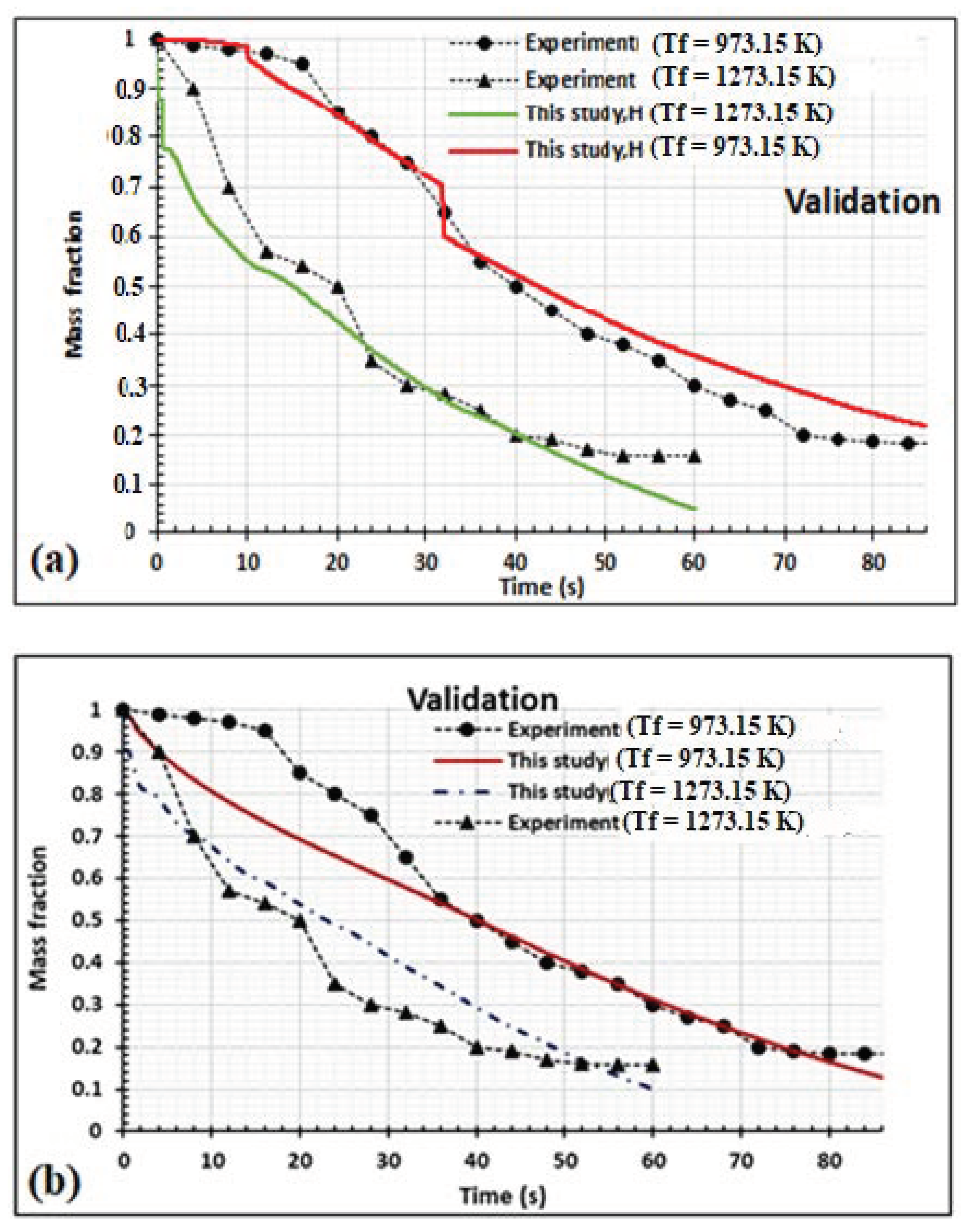
Assumptions	Tf = 973.15 K		Tf = 1273.15 K
	MAE (-)	MRE (%)	MAE (-)	MRE (%)
Dry wood	0.066	10.376	0.065	22.632
Humid wood (0.25 kg/kg moisture content)	0.028	10.181	0.041	14.735

), showing a closer association and better results with the experimental data, as shown in Figure 4b. All the mean absolute error values are lower than 0.1, and the mean relative error value at 973.15 K is close to 10%. When the oven temperature is equal to 1273.15 K, the mean relative error value is greater than 10%, which might be a result of the high volatility of the volatile mass fraction. Again, differences can be explained by the geometrical form of the experimental samples used to generate the experimental data and the parallelepiped geometry modeled, which can be influenced by the assumptions applied in the numerical model. In effect, Bonnefoy et al. [38] used cubic wood samples heated on all six sides; however, in this case, we assumed that the samples were dried and heated on two main axes. The thermo-physical parameters used in our model might also influence the variation obtained. The presence of moisture content in the samples decreases the kinetics of thermal degradation, as shown by the experimental data used [38] and confirmed in previous works [31]. It took about 100 s to complete the pyrolysis of 30 mm parallelepiped wood at 973.15 K, and about 60 s for 1273.15 K. Comparatively, this time is similar to the pyrolysis of 20 mm spherical wood chip in the same temperature range, but lower than the time taken for pyrolysis of 20 mm height and 20 mm diameter cube and cylindrical wood chips, respectively [16,19]. Comparatively, the pyrolysis of parallelepiped wood is shorter because of its higher thickness. However, Areya et al. [19] did not state the type of wood they used, although they stated it was randomly selected.

The temperature evolution is shown in Figure 5. From Figure 5a, the wood core temperature began to increase after 6 s. However, the influence of the initial moisture content on the temperature evolution of the product at the wood core was not seen until 30 s of heating. During this period, temperature propagation at the center was slow, and the reaction was endothermic, leading to high solid mass loss [21]. This corresponds to the decomposition of high volatiles like cellulose in the primary reaction scheme. After 30 s, the heating front generally increased steeply, but the dried samples with lower initial moisture content moved up rapidly compared to samples with higher moisture content. According to Park et al. [21], this exothermic reaction period is when the intermediate solids are converted to biochar. However, the difference in temperature evolution between the samples with lower moisture and those with high moisture is because some of the heat is absorbed by the moisture for evaporation in the case of samples with high moisture content. This has also been observed by Pozlon et al. [39]. Thus, the moisture content in the product decreases the kinetics of the pyrolysis process. Figure 5b shows that moisture content at the center of the product decreased after 80 s, 90 s, and 98 s for all initial temperatures. Thus, using the same energy for the process, samples with high initial moisture content have a kinetic degradation lower than those with lower initial moisture content.

Figure 6 presents the numerical results for the densities of wood decomposed to produce charcoal, tar, and gas. The 30 mm thick samples were heated on two sides at 973.15 K and completely pyrolyzed after 900 s. Some part of tar was transformed into gas and biocharcoal during secondary reactions. At the end of the process, the density of biocharcoal produced was 600 kg/m³,while the density of tar and gas was 44 kg/m³ and 74 kg/m³, respectively. It is important to note that the gas produced is a mixture of gas species, as specified by literature [31,40]. After 675 s of the process, the density of tar becomes constant. Gas and char produced after 675 s are directly due to the decomposition of the wood. Figure 7 presents the evolution of the temperature of wood when the temperature of the oven is equal to 973.15 K. This evolution increases during the process, but the internal temperature of the wood remains lower than the temperature of the oven. In effect, the exterior faces of the samples rapidly reached the value of the temperature of the oven (Figure 8), but the temperature of the interior parts of the samples increased progressively with time, as noticed in the literature [26,31]. This is confirmed in Figure 8, which shows the variation of temperature with time for the wood sample heated to Tf = 973.15 K, at both extremities. The pyrolysis front moves from the surface, through which the sample is heated, towards the center of the sample. The propagation of the conductive wave, through the heated wood, increases the temperature in the center as time passes. The analysis of the curve shows a symmetrical evolution to the center, suggesting the possibility of studying the phenomenon in one half of the sample. From the start of the process to 850 s, the temperature of the center of the sample increases from 293.15 K to 460 K, but at the surfaces, the temperature increases from 293.15 K to 925 K. This is due to the low value of the thermal conductivity of the wood. The pressure distribution of the volatile products is shown in Figure 9 and varies between 1 to 4.5 p/po. The pressure increases from the surfaces to the center once the time of the process reaches 375 s. The pressure of gases in the samples is influenced by the temperature gradients. When the gradients of temperature are neglected, as shown between 0.01 m and 0.02 m of the samples for time duration lower than 375 s, the pressure decreases to zero. As time increases, the wood is fully subjected to pyrolysis, and the pressure increases until it becomes uniform. The reduction of the pressure of the gas in the wood chips increases the degradation of the wood and the degradation of the biochar produced during the process. Park et al. [21] obtained similar results for pressure varying between 1 to 1.6 p/po during pyrolysis of wood biomass at 1180 K. Cai et al. [41] concluded that the reactivity (or activation energy) of biochar decreases when the pressure fraction increases to 20 atm, and then increases when the pressure fraction increases to a higher pressure, up to 15 atm. Thus, to optimize the production of biochar, the pressure fraction during the process must be low.

Figure 8 and Figure 9 show that the temperature and pressure of volatile products vary together.

Figure 10 presents the evolution of the velocity of the gas in the sample during the process when the two main sides of the samples are heated at 973.15 K. We saw that this evolution is not regular and is lower than 7 × 10⁻⁶ m/s. When x = 0.03 m, we assume that the gradients of velocity and pressure are equal to zero, assuming that the samples are not permeable on this side. This condition permits the neglect of the flux of volatile products on this side (x = 0.03 m). Figure 11 presents the distributions of biocharcoal during the process according to the wood thickness when the temperature of the oven is equal to 973.15 K. The biochar is produced from the surface to the core of the wood samples. When the process continues, charcoal is produced in the center but transformed into other products around the surface of the product. Only 5 mm of each side is destroyed.

In Figure 12, Figure 13 and Figure 14, the side x = 0.0 m and side x = 0.03 m are respectively heated at T_f1 = 773.15 K and T_f2 = 973.15 K, but the heat flux density is equal to zero. This non-symmetrical heating is compared to symmetrical heating when the heat flux density is equal to zero. Figure 12 presents the wood temperature evolution at 850 s. As shown in Figure 13, when the temperature increases, the pressure of volatile products also increases in all thicknesses of the samples. The pressure fraction increases from the surface to the center. In effect, as showed by Zeng [41], temperature evolution in the product decreases when the wood pressure increases. Figure 14 shows that when the temperature increases, the biocharcoal production also increases, but a part of the biocharcoal near the surface is also transformed into other products, such as ash. Thus, it is clearly important to have a temperature where the produced biocharcoal is optimal.

Figure 15, Figure 16 and Figure 17 present the influences of temperature and heat flux density on the pyrolysis process and the produced biocharcoal. A comparison is done with the case where the heating is symmetrical and flux heat density is equal to zero. This comparison is done when the processing time is 850 s. Figure 15 shows that the heat flux density increases the value of the temperature on all the thicknesses of the sample. This heat flux density also influences the pressure of the volatile products produced during the pyrolysis process, as shown in Figure 16. Figure 17 showed that the heat flux density influences the production of biocharcoal. When the heat flux density increases, the production of biocharcoal in the inner portion of the sample also increases, but the destruction of the biocharcoal on the surface of the sample is progressive. Cai et al. [42] had obtained the same evolutions of the pressure during the pyrolysis process and concluded that to optimize the production of biochar, the pressure fraction during the process must be weak. Thus, they found that combustion reactivity decreased during hydro-pyrolysis at pressure up to 40 atm and increased at pressures above 40 atm [42]. Sha et al. [43] had noted the decrease of combustion reactivity as pressure increases. Thus, it is clear that the parts in Figure 13 where pressure is high (in the center of the product) have more biochar than the parts where the pressure is weak. Figure 14 confirms this perception, because the density of the biochar is higher in the center of the product than in the surface where the combustion process is high. Figure 15, Figure 16 and Figure 17 confirm the results obtained by Cai et al. [42], Sha et al. [43], and Van Heek and Mühlen [44] for inert conditions of pyrolysis. Variation of pressure must be integrated during the pyrolysis process, because many models did not take into account the effect of pressure during pyrolysis [45].

4. Conclusions

The model of Di-Blasi and Russo [14] was used to explain the pyrolysis process of parallelepiped-shaped wood, and the effect of moisture content was studied using a modified Di-Blasi and Russo model established in this study. Using a modeling and simulation approach to the pyrolysis process, it was shown that the density of wood decreases, while densities of gas, charcoal, and tar increase, showing their production. The average final densities of gas, charcoal, and tar obtained are 74 kg/m³, 600 kg/m³, and 44 kg/m³, respectively. The pressure of volatile products, temperature, and rates of production of charcoal, gas, and tar increased from the heated surface to the center of the sample. The heat flux density increased the degradation of the wood. Results obtained show that the charcoal produced near the surface can be destroyed when the temperature of the oven and the heat flux density are not well chosen.

References

- Simo-Tagne, M.; Ndukwu, M.C.; Ndi-Azese, M. Experimental Modelling of a Solar Dryer for Wood Fuel in Epinal (France). Modelling 2020, 1, 39–52. [Google Scholar] [CrossRef]
- Simo-Tagne, M.; Rémond, R.; Rogaume, Y.; Zoulalian, A.; Perré, P. Characterization of sorption behaviour and mass transfer properties of four central African tropical woods: Ayous, Sapele, frake, lotofa. Maderas. Cienc. Tecnol. 2016, 18, 207–226. [Google Scholar]
- Simo-Tagne, M.; Rémond, R.; Rogaume, Y.; Zoulalian, A.; Bonoma, B. Sorption behaviour of four tropical woods using a dynamic vapour sorption standard analysis system. Maderas Cienc. Tecnol. 2016, 18, 403–412. [Google Scholar]
- Simo-Tagne, M. Experimental characterization of the influence of water content on the density and shrinkage of tropical woods coming from Cameroon and deduction of their fiber saturation points. Int. J. Sci. Res. 2014, 3, 510–515. [Google Scholar]
- Prakash, N.; Karunanithi, T. Kinetic modelling in biomass pyrolysis—A review. J. Appl. Sci. Res. 2008, 4, 1627–1636. [Google Scholar]
- Anca-Couce, A.; Sommersacher, P.; Scharler, R. Online experiments and modelling with a detailed reaction scheme of single particle biomass pyrolysis. J. Anal. Appl. Pyrolysis 2017, 127, 411–425. [Google Scholar] [CrossRef]
- Solanki, S.; Baruah, B.; Tiwari, P. Modeling and simulation of wood pyrolysis process using COMSOL Multiphysics. Bioresour. Technol. Rep. 2022, 17, 100941. [Google Scholar] [CrossRef]
- Ndukwu, M.C.; Horsfall, I.T. Prospects of Pyrolysis Process and Models in Bioenergy Generation: A Comprehensive Review. Polytechnica 2020, 3, 43–53. [Google Scholar] [CrossRef]
- Ndukwu, M.C.; Horsfall, I.T.; Ubouh, E.A.; Orji, F.N.; Ekop, I.E.; Ezejiofor, N.R. Review of solar-biomass pyrolysis systems: Focus on the configuration of thermal-solar systems and reactor orientation. J. King Saud Univ. Eng. Sci. 2021, 33, 413–423. [Google Scholar] [CrossRef]
- Pecha, M.P.; Arbelaez, J.I.M.; Garcia-Perez, M.; Chejne, F.; Ciesielski, P.N. Progress in understanding the four dominant intra-particle phenomena of lignocelluloses pyrolysis: Chemical reactions, heat transfer, mass transfer, and phase change. Green Chem. 2019, 21, 2868–2898. [Google Scholar] [CrossRef] [Green Version]
- Suopajärvi, H.; Umeki, K.; Mousa, E.; Hedayati, A.; Romar, H.; Kemppainen, A.; Chuan Wang, C.; Phounglamcheik, A.; Tuomikoski, S.; Norberg, N.; et al. Use of biomass in integrated steelmaking—Status quo, future needs and comparison to other low-CO2 steel production technologies. Appl. Energy 2018, 213, 384–407. [Google Scholar] [CrossRef] [Green Version]
- Phounglamcheik, A.; Wang, L.; Romar, H.; Kienzl, N.; Broström, M.; Ramser, K.; Skreiberg, Ø; Umeki, K. Effects of Pyrolysis Conditions and Feedstocks on the Properties and Gasification Reactivity of Charcoal from Woodchips. Energy Fuels 2020, 34, 8353–8365. [Google Scholar] [CrossRef]
- Mellin, P.; Kantarelis, E.; Yang, W. Computational fluid dynamics modelling of biomass fast pyrolysis in a fluidized bed reactor, using a comprehensive chemistry scheme. Fuel 2014, 117, 704–715. [Google Scholar] [CrossRef]
- Jin, H.Z.; Zhen, B.W.; Hui, Z.; Yuan, Y.T.; Hong, H.S.; Chao, H.Y. Multi-scale CFD simulation of hydrodynamics and cracking reactions in fixed fluidized bed reactors. Appl. Petrochem. Res. 2015, 5, 255–261. [Google Scholar] [CrossRef] [Green Version]
- Hiroki, H.; Hiroomi, H.; Muhammad, I. Numerical Analysis on Wood Pyrolysis in Pre-Vacuum Chamber. J. Sustain. Bioenergy Syst. 2014, 4, 149–160. [Google Scholar]
- Assoumani, N.; Simo-Tagne, M.; Kifani-Sahban, F.; Tagne Tagne, A.; El Marouani, M.; Obounou Akong, M.B.; Rogaume, Y.; Girods, P.; Zoulalian, A. Numerical study of cylindrical tropical woods pyrolysis using python tool. Sustainability 2021, 13, 13892. [Google Scholar] [CrossRef]
- Pang, S. Advances in thermochemical conversion of woody biomass to energy, fuels and chemicals. Biotechnol. Adv. 2019, 37, 589–597. [Google Scholar] [CrossRef]
- Okekunle, P.O.; Adunola, V.L.; Whanvoh, E.S.; Afolabi, A.P.; Idiok, E.P. Experimental Investigation of the Effect of Sample Shape on Biomass Pyrolysis Characteristics in a Fixed Bed Reactor. J. Nat. Sci. Res. 2015, 5, 120. [Google Scholar]
- Atreya, A.; Olszewski, P.; Chen, Y.; Baum, H.R. The effect of size, shape and pyrolysis conditions on the thermal decomposition of wood particles and firebrands. Int. J. Heat Mass Transf. 2017, 107, 319–328. [Google Scholar] [CrossRef]
- Gentile, G.; Debiagi, P.E.A.; Cuoci, A.; Frassoldati, A.; Ranzi, E.; Faravelli, T. A computational framework for the pyrolysis of anisotropic biomass particles. Chem. Eng. J. 2017, 321, 458–473. [Google Scholar] [CrossRef]
- Park, W.C.; Atreya, A.; Baum, H.R. Experimental and theoretical investigation of heat and mass transfer processes during wood pyrolysis. Combust. Flame 2010, 157, 481–494. [Google Scholar] [CrossRef]
- Baltrušaitis, A.; Pranckevičienė, V. The Influence of Log Offset on Sawn Timber Volume Yield. Mater. Sci. 2005, 11, 403–406. [Google Scholar]
- WoodChipIstock. Available online: https://www.istockphoto.com/photos/wood-chip (accessed on 1 March 2022).
- Simo-Tagne, M. Contribution à L’étude du Séchage des Bois Tropicaux au Cameroun: Aspects Caractérisation, Modélisation Multi-Echelle et Simulation, le Cas des Bois D’ayous (Triplochiton scleroxylon) et D’ébène (Diospyros crassiflora). Ph.D. Thesis, University of Yaoundé I, Yaoundé, Cameroon, 2011. [Google Scholar]
- Oumarou, N.; Kocaefe, D.; Kocaefe, Y. 3D-modelling of conjugate heat and mass transfers: Effects of storage conditions and species on wood high-temperature treatment. Int. J. Heat Mass Transf. 2014, 79, 945–953. [Google Scholar] [CrossRef]
- Thi, V.D. Modélisation du Comportement au Feu des Structures en Bois. Ph.D. Thesis, University of Lorraine, Epinal, France, 2017. [Google Scholar]
- Simo-Tagne, M.; Zoulalian, A.; Rémond, R.; Rogaume, Y. Mathematical modelling and numerical simulation of a simple solar dryer for tropical wood using a collector. Appl. Therm. Eng. 2018, 131, 356–369. [Google Scholar] [CrossRef]
- Di-Blasi, C.; Russo, G. Modelling of transport phenomena and kinetics of biomass pyrolysis. In Advances in Thermochemical Biomass Conversion; Bridgwater, A.V., Ed.; Blackie Academic and Professional: New York, NY, USA, 1994; pp. 906–921. [Google Scholar]
- Di-Blasi, C. Analysis of convection and secondary reaction effects within porous solid fuels undergoing pyrolysis. Combust. Sci. Technol. 1993, 90, 315–340. [Google Scholar] [CrossRef]
- Simpson, W.; Tenwold, A. Physical properties and moisture relations of wood. In Wood Handbook: Wood as an Engineering Material; USDA Forest Service, Forest Product Laboratory: Madison, WI, USA, 1999; Volume 3, pp. 1–23. [Google Scholar]
- Yuen, R.; Casey, R.; De-Vahl-Davis, G.; Leonardi, E.; Yeoh, G.H.; Chandrasekaran, V.; Grubits, S.J. A three-dimensional mathematical model for the pyrolysis of wet wood. Intl. Assoc. Fire Saf. Sci. 1997, 5, 189–200. [Google Scholar] [CrossRef] [Green Version]
- Christodoulou, M. Pyrolyse du Bois dans les Conditions d’un Lit Fruidisé: Étude Expérimentale et Modélisation. Ph.D. Thesis, University of Lorraine, Lorraine, France, 29 November 2013. [Google Scholar]
- Chan, W.C.; Kelbon, M.; Krieger, B.B. Modelling and experimental verification of physical and chemical processes during pyrolysis of a large biomass particle. Fuel 1985, 64, 1505–1513. [Google Scholar] [CrossRef]
- Bryden, K.M.; Hagge, M.J. Modeling the combined impact of moisture and char shrinkage on the pyrolysis of a biomass particle. Fuel 2003, 82, 1633–1644. [Google Scholar] [CrossRef]
- Glaister, D.S. The Prediction of Chemical Kinetics, Heat and Mass Transfer Processes during the One- and Two-Dimensional Pyrolysis of a Large Woof Pellets; Université de Washington: Washington, DC, USA, 1987. [Google Scholar]
- Liedtke, A. Etude Cinétique du Séchage du Bois dans un Four à Image; Rapport de Projet de Fin d’Etude; LSGC, CNRS-Nancy Université: Nancy, France, 2008. [Google Scholar]
- Svenson, J.; Pettersson, J.B.C.; Davidsson, K.O. Fast pyrolysis of the main components of birch wood. Combust. Sci. Technol. 2004, 176, 977–990. [Google Scholar] [CrossRef]
- Bonnefoy, F.; Gilot, P.; Prado, G. A three-dimensional model for the determination of kinetic data from the pyrolysis of beech wood. J. Anal. Appl. Pyrolysis 1993, 2, 387–394. [Google Scholar] [CrossRef]
- Pozzobon, V.; Salvador, S.; Bézian, J.J.; El-Hafi, M.; Le-Maoult, Y.; Flamant, G. Radiative pyrolysis of wet wood under intermediate heat flux: Experiments and modelling. Fuel Processing Technol. 2014, 128, 319–330. [Google Scholar] [CrossRef] [Green Version]
- Horsfall, I.T.; Ndukwu, M.C.; Abam, F.; Simo-Tagne, M.; Nwachukwu, C.C. Parametric studies of heat and mass transfer process for two-stage biochar production from poultry litter pellet biomass. Biomass Convers. Biorefnery 2022, 1–13. [Google Scholar] [CrossRef]
- Zeng, D. Effects of Pressure on Coal Pyrolysis at High Heating Rates and Char Combustion. Ph.D. Thesis, Brigham Young University, Provo, UT, USA, 2005. [Google Scholar]
- Cai, H.Y.; Guell, A.J.; Chatzakis, I.N.; Lim, J.Y.; Dugwell, D.R.; Kandiyoti, R. Combustion Reactivity and Morphological Change in Coal Chars: Effect of Pyrolysis Temperature, Heating Rate and Pressure. Fuel 1996, 75, 15–24. [Google Scholar] [CrossRef]
- Sha, X.Z.; Chen, Y.G.; Cao, J.; Yang, Y.M.; Ren, D.Q. Effects of Operating Pressure on Coal Gasification. Fuel 1990, 69, 293. [Google Scholar] [CrossRef]
- Van-Heek, K.H.; Muhlen, H.-J. Fundamental Issues in Control of Carbon Gasification Reactivity; Kluwer Academic Publishers: Dordrecht, The Netherlands, 1991. [Google Scholar]
- Xia, C.; Cai, L.; Zhang, H.; Zuo, L.; Shi, S.Q.; Lam, S.S. A review on the modeling and validation of biomass pyrolysis with a focus on product yield and composition. Biofuel Res. J. 2021, 29, 1296–1315. [Google Scholar] [CrossRef]