
An Agent-Based Model of Heterogeneous Driver Behaviour and Its Impact on Energy Consumption and Costs in Urban Space

 , , , , , and
Abstract
1. Introduction
2. Background
3. Model Description
3.1. Purpose
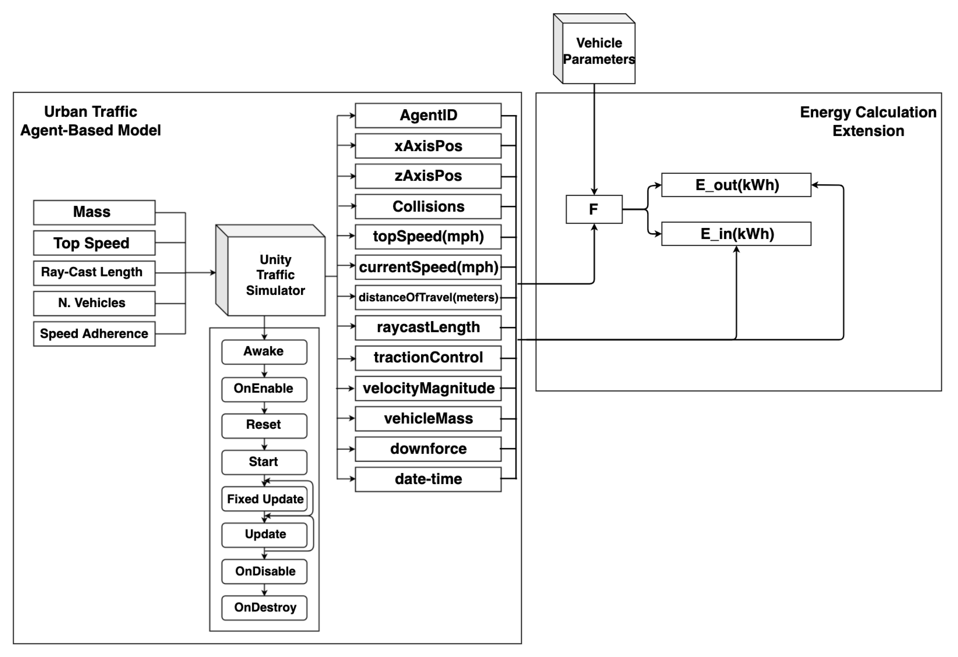
3.2. Variables
- The vehicle mass parameter, drawn from a random uniform distribution between 1000 and 3000 kg (inclusive), allows the model to simulate a wider variety of vehicle types, from sedans to SUVs and hatchback. The rationale behind this distribution was to try intersect the EV and ICEV vehicle types, which larger vehicles such as vans or trucks are not part of; the model distributes vehicles arbitrarily across the environment with varying weights (source [39]).
- The top speed measure is between 30 and 45 mph (48, 72 km/h) and is only applied to vehicles that do not adhere to speed limits. This measure is applied only if Speed Adherence is ≥1 (source [40]).
- The gap acceptance parameter can be between 1 to 10 for each vehicle. The variable assigns a distance between two vehicles in meters. This ensures a wider variety of visual impairment is captured as some people with healthier eyes keep a fair distance from vehicles in front usually adhering to the 2-s rule compared to people with worse vision. Furthermore, the distance had to be relative to the average road distance in the model.
- The number of vehicles generated in the model, N. This can be between 1 and 500. However, this can be adjusted depending on the compute power accessible. The hardware accessible at the time of writing this article could only efficiently simulate up to 500 vehicles in 3D space while yielding valid results (refer to the Conclusions section for more on this limitation).
- The speed adherence variable can be between . This quantifies the proportion of vehicles that will not adhere to the speed limits applied to the road they are driving on.
- The urban road network consists of 1295 roads which vehicles drive on and 354 intersections which consist of traffic rules (Algorithm 1, Ref. [28]). The road network has been designed to depict a small urban town.
3.3. Model Overview
3.4. Agent
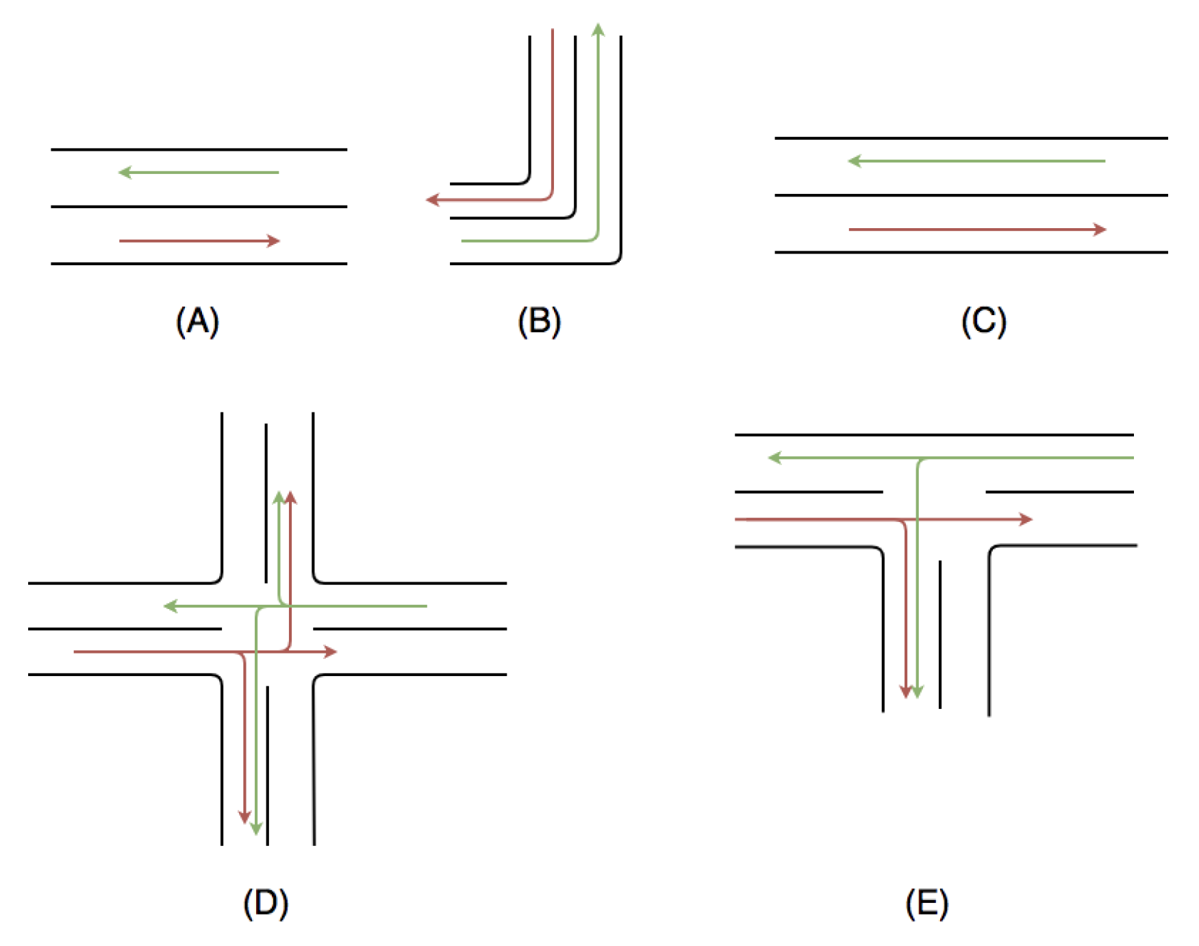
3.5. Environment
- (A) A two-way local road with a speed limit of 20 mph (32 km/h);
- (B) A two-way corner road with a speed limit of 10 mph (16 km/h);
- (C) A two-way fixed road with a speed limit of 30 mph (48 km/h);
- (D) An eight-way intersection. Right-of-way is for traffic on horizontal lanes, and the speed limit is 10 mph (16 km/h);
- (E) A two-way t-junction. Right-of-way is for horizontal lanes, and the speed limit is 10 mph (16 km/h).
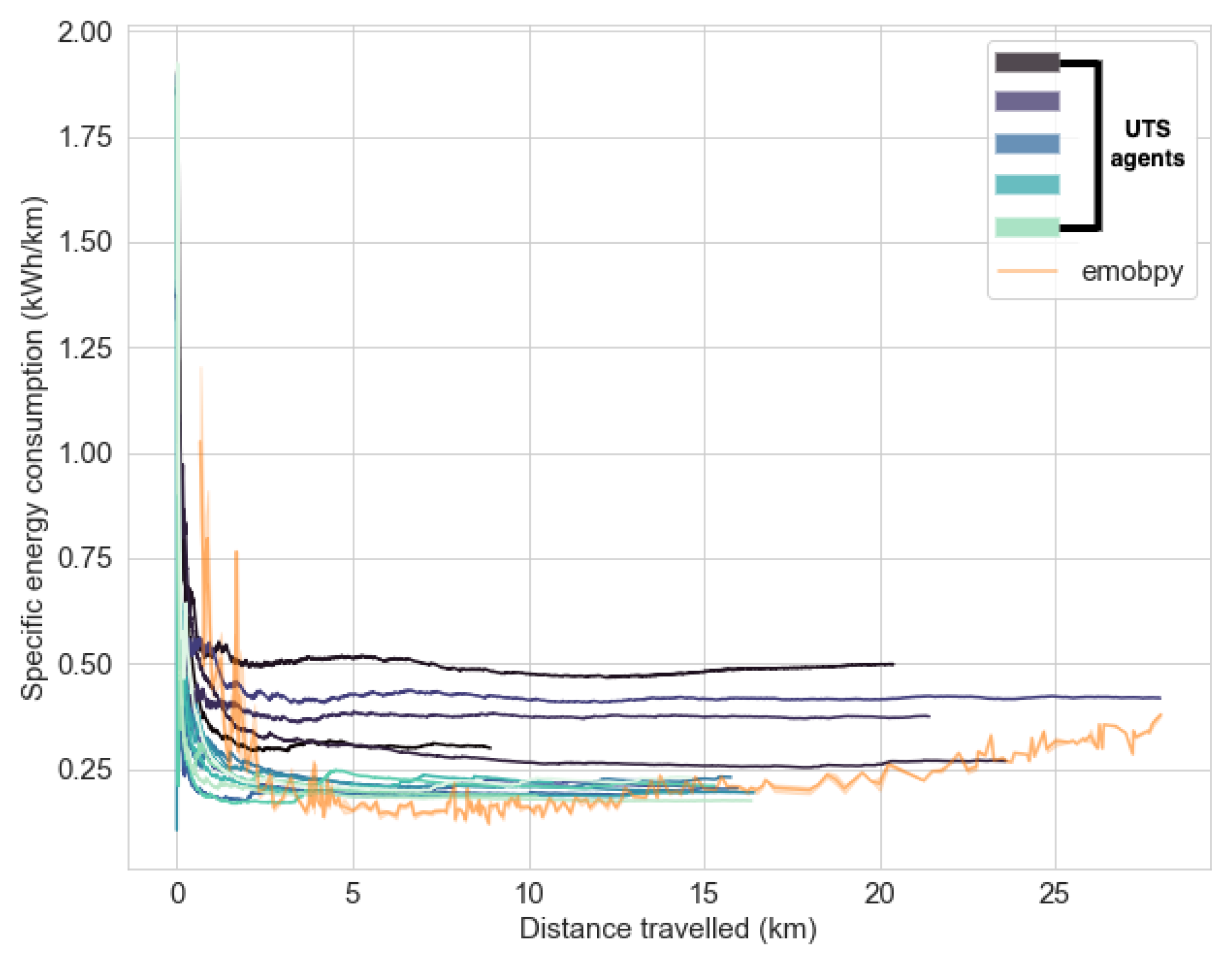
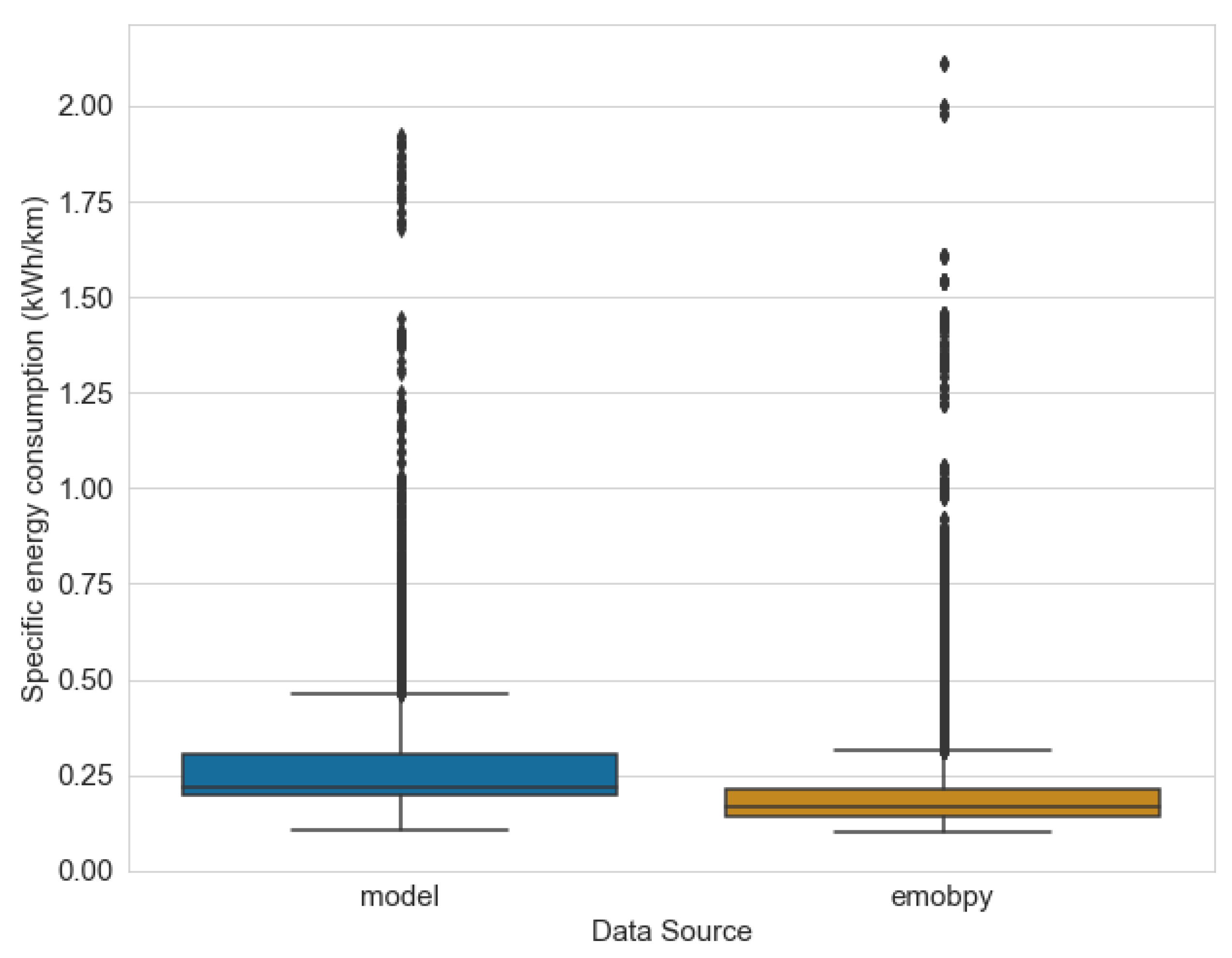
4. Results
- That it produces outputs at a time resolution of 15 min; our model, on the other hand, has a time resolution of 1 s. This way, we can capture finer detail such as the impact of traffic lights on acceleration/deceleration and momentary traffic congestion;
- That it only captures trips that are split into commuters and non-commuters. Thus, the modelled scenarios revolve around two profiles of drivers. Our model manipulates the entire system from the street network to traffic rules and vehicles; thus, no single driver profile is modelled, but a heterogeneous set of behaviours are captured.
4.1. Electric Energy Consumption Calculation
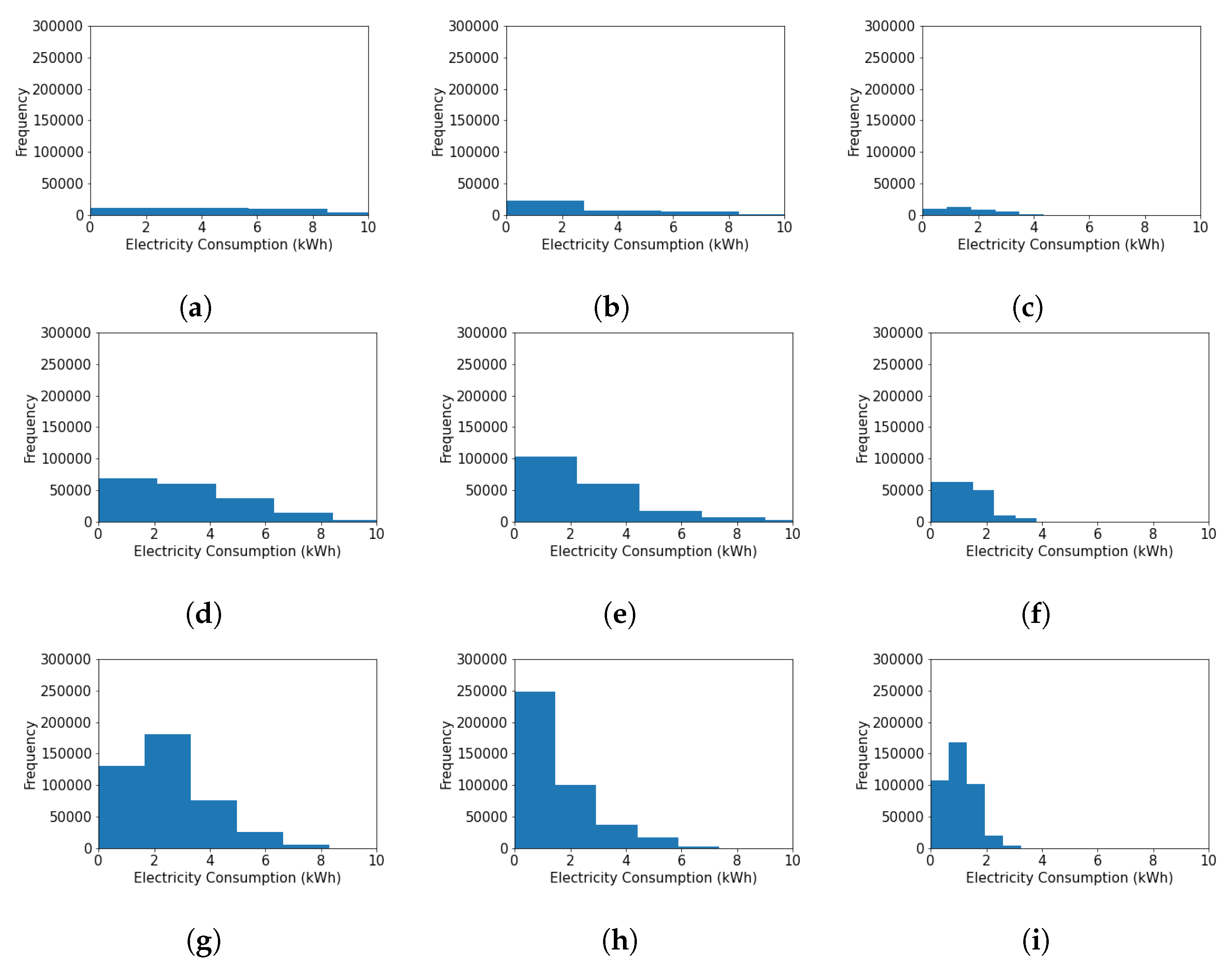
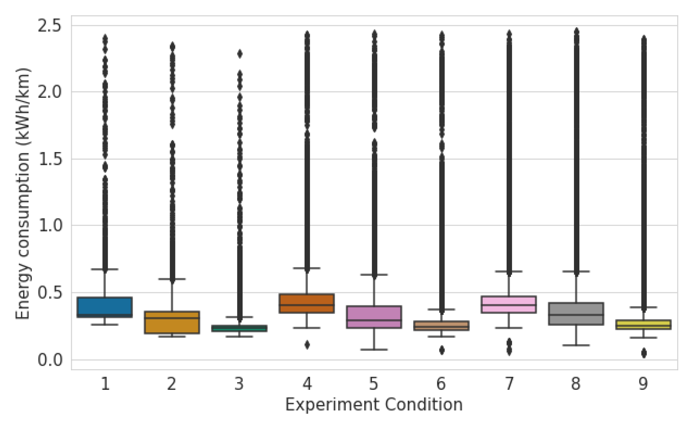
4.2. Experiments
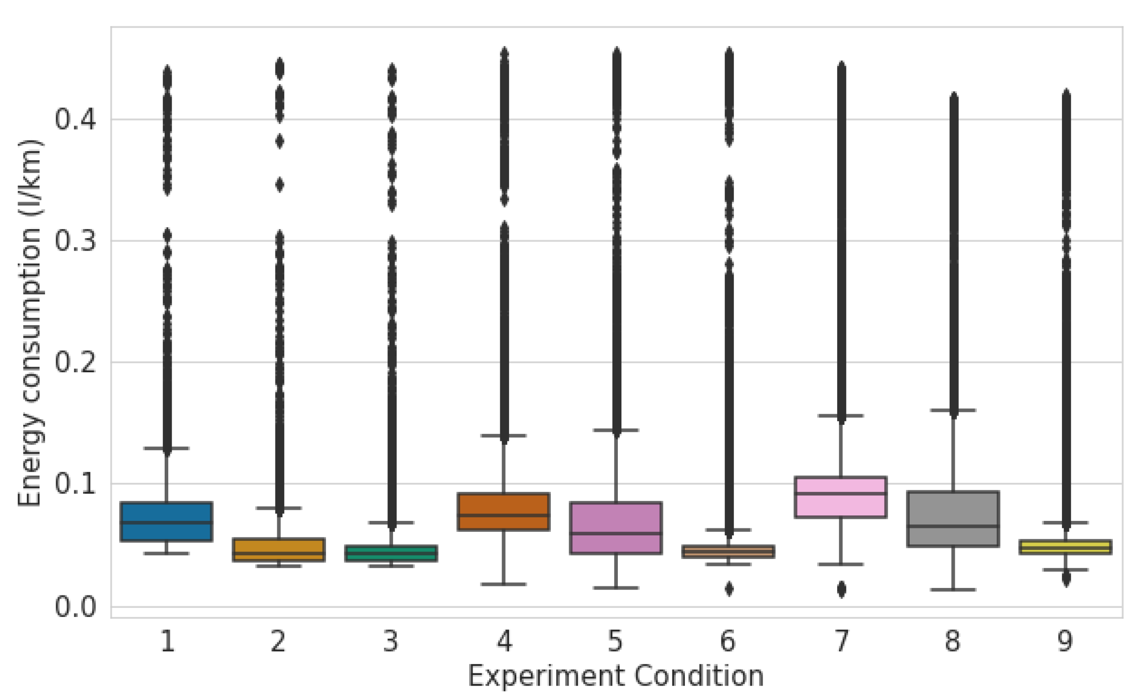
4.2.1. Fuel Consumption of Internal Combustion Engine Vehicle Fleet
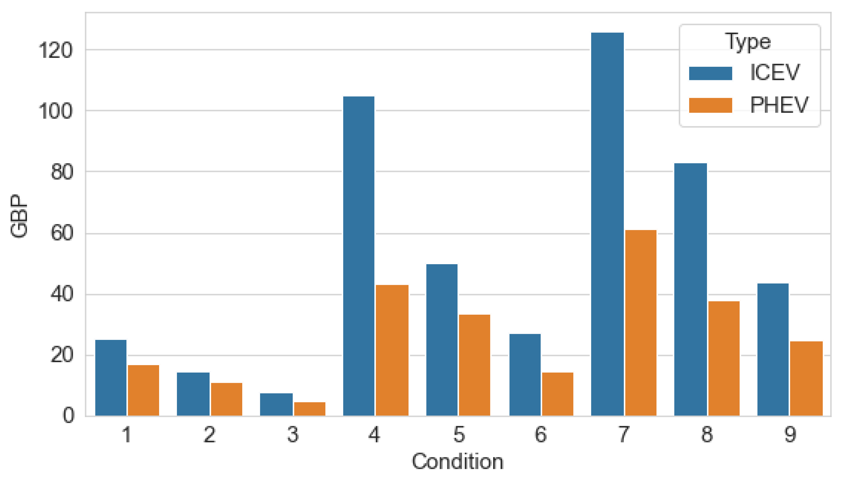
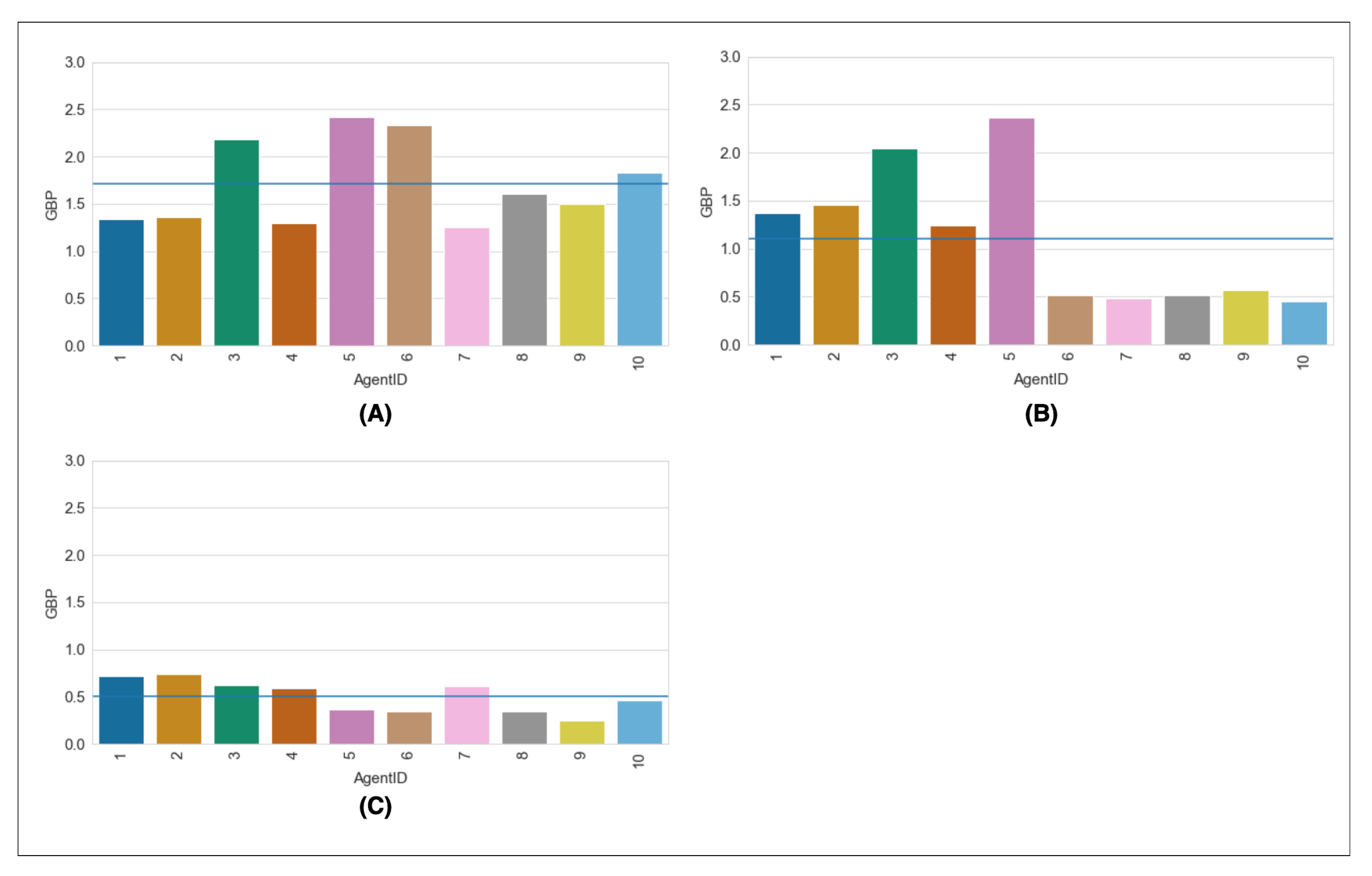
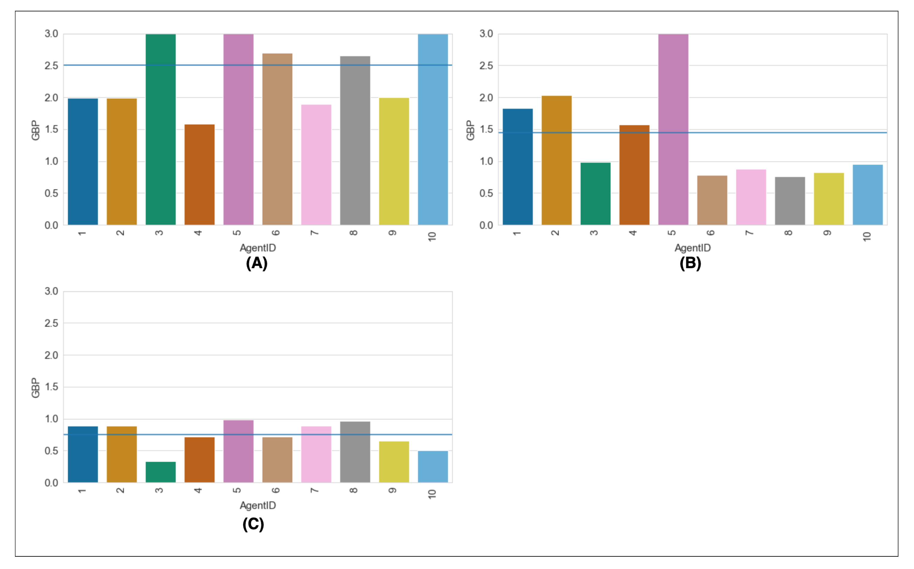
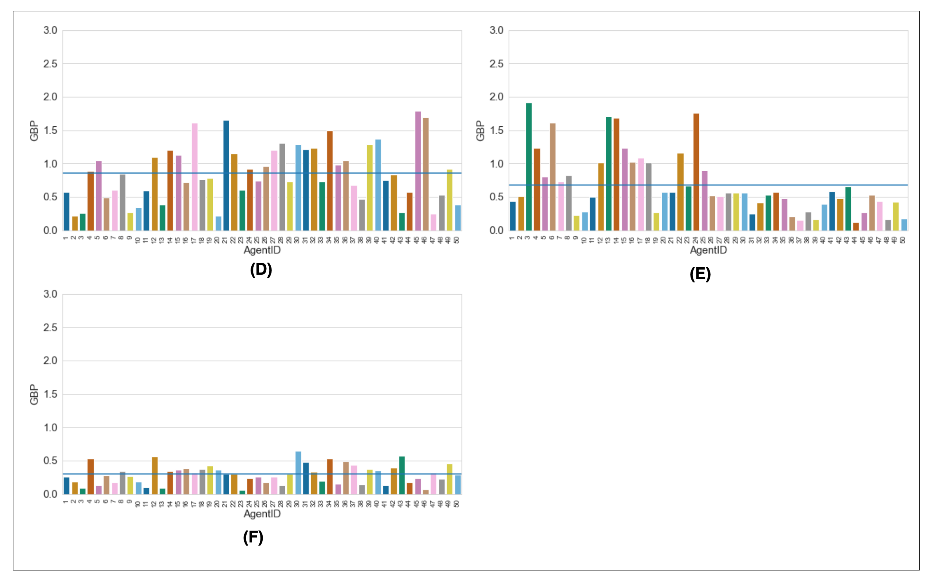
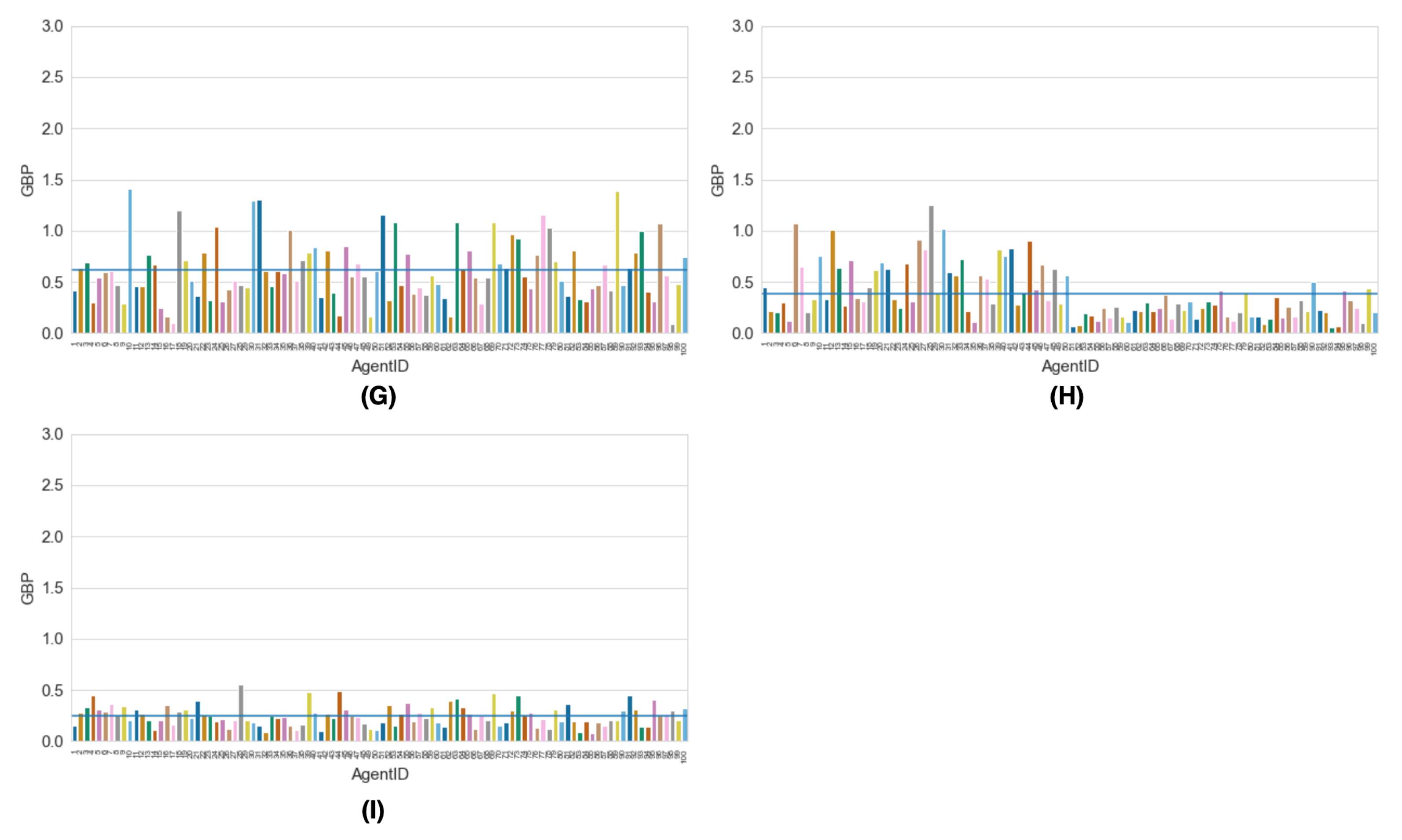
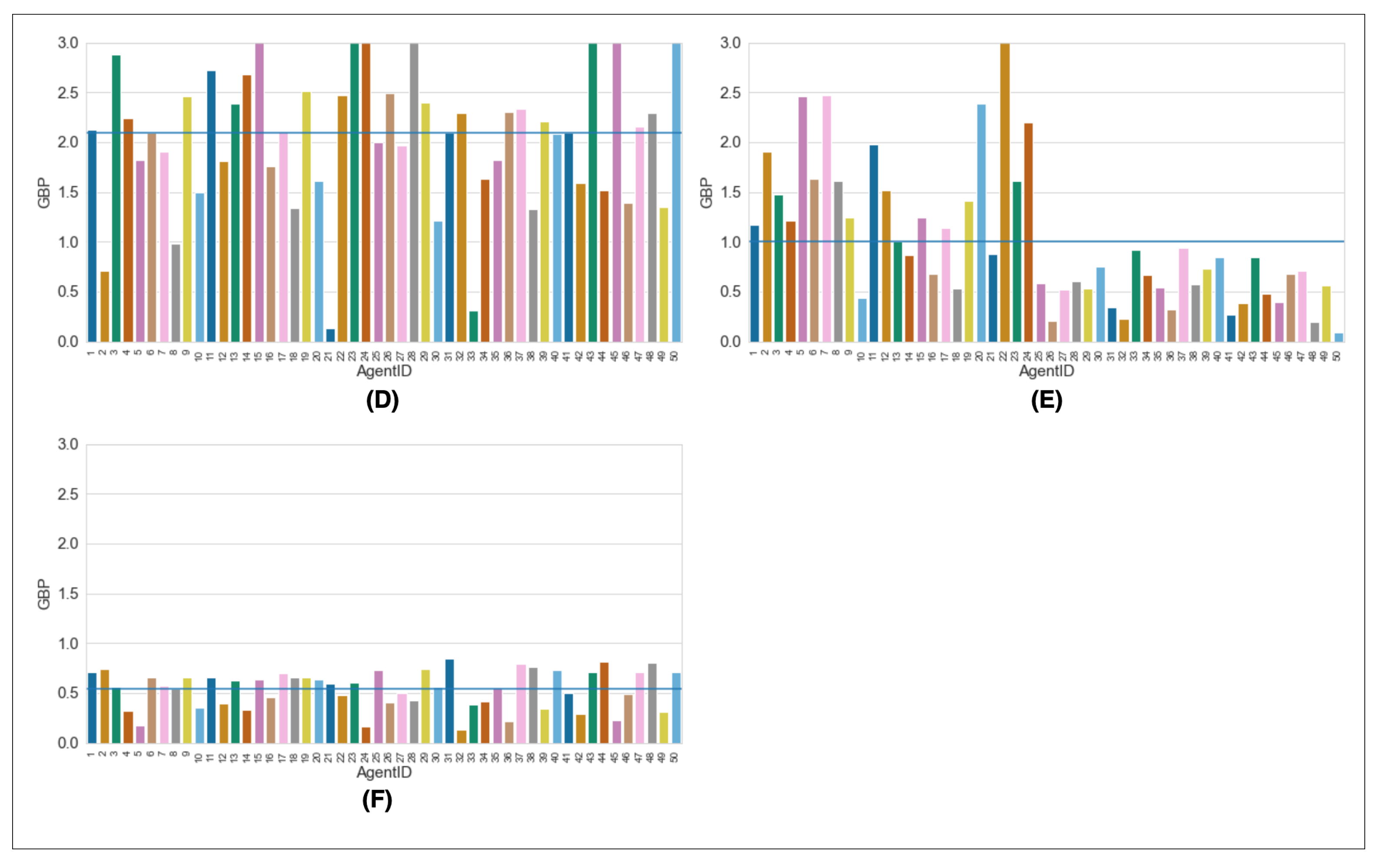
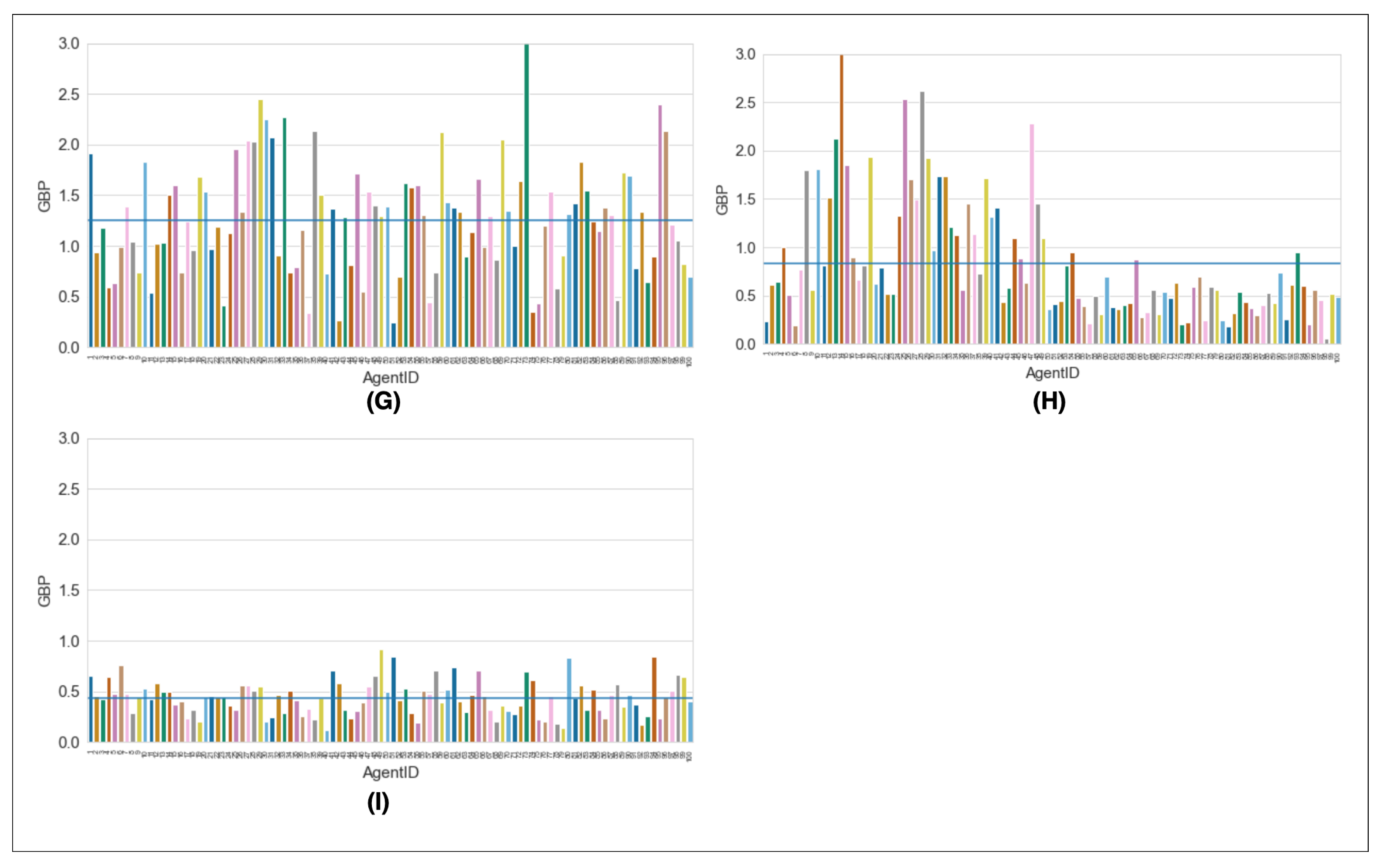
4.2.2. Monetary Costs of Fuel and Electric Consumption
5. Discussion
6. Conclusions
Author Contributions
Funding
Institutional Review Board Statement
Informed Consent Statement
Data Availability Statement
Conflicts of Interest
Appendix A
Appendix A.1. Energy Calculation
- F is the force provided by the engine driving the vehicle forward (N);
- m is the mass of the vehicle (kg);
- g is the gravitational acceleration (m/s2);
- is the angle of the surface on which the vehicle is driving on;
- is the density of air (1.225 kg/m3);
- is the drag coefficient;
- A is the reference area of the vehicle (m2) (width × height);
- v is the velocity (m/s), and;
- is the coefficient of rolling resistance.
Appendix B
Tables

| Variable | Output Type |
|---|---|
| VelocityChange | Float |
| Acceleration | Float |
| Deceleration | Float |
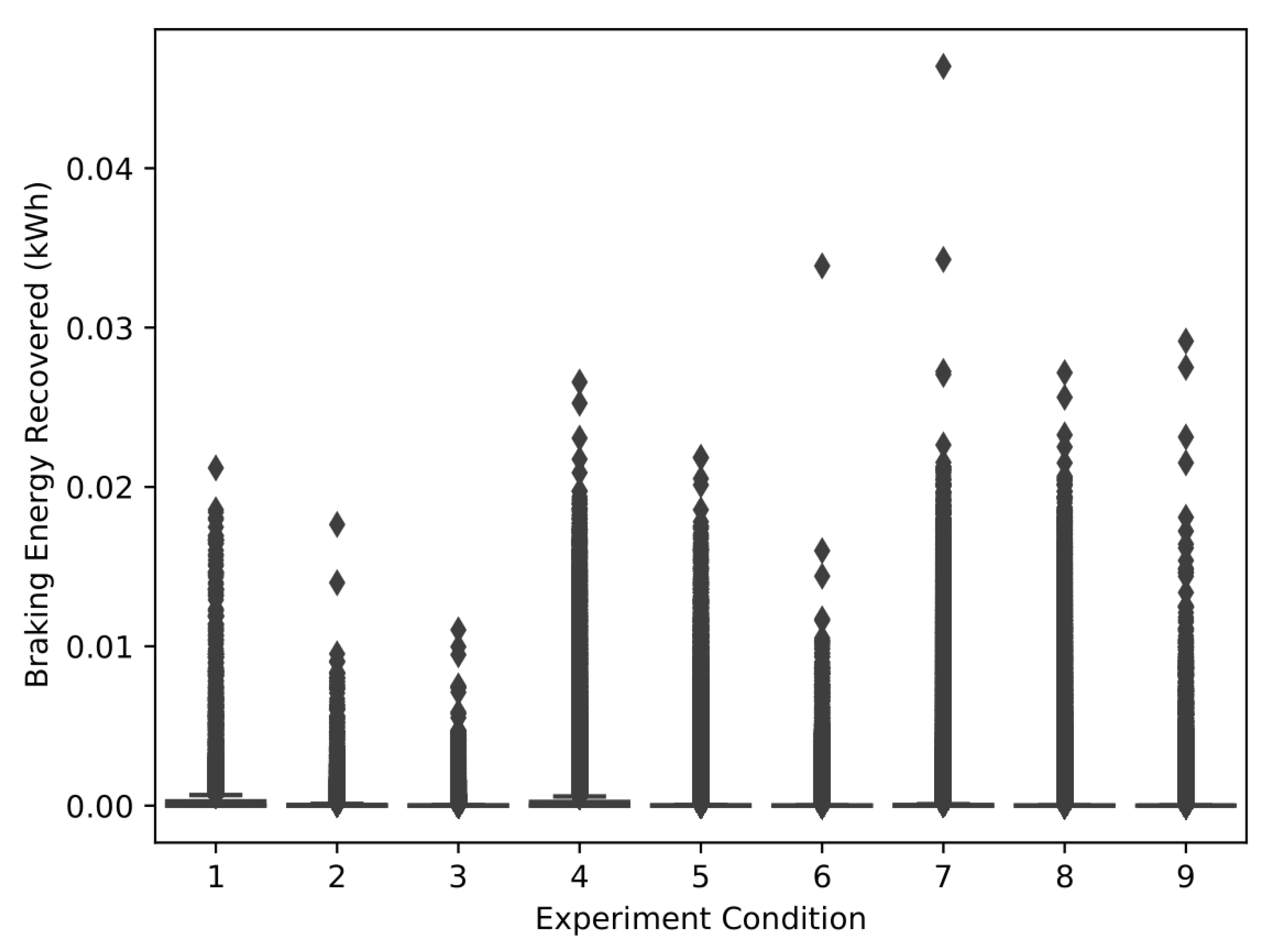
| Braking Energy (kWh) 1 | Float |
| Drag_Force | Float |
| Acceleration_Force | Float |
| Total_Force | Float |
| Drag_Work | Float |
| Acceleration_Work | Float |
| Total_Work | Float |
| Energy_Input (kWh) | Float |
| Energy_Input_Sum (kWh) | Float |
| MC | PHEV | ICEV |
|---|---|---|
| 1 | 0.60 | 0.92 |
| 2 | 0.43 | 0.56 |
| 3 | 0.22 | 0.34 |
| 4 | 1.93 | 4.42 |
| 5 | 1.50 | 2.25 |
| 6 | 0.67 | 1.22 |
| 7 | 2.79 | 5.66 |
| 8 | 1.72 | 3.71 |
| 9 | 1.12 | 1.98 |
Appendix C
Appendix C.1. Figures


References
- Bretzke, W.R. Global urbanization: A major challenge for logistics. Logist. Res. 2013, 6, 57–62. [Google Scholar] [CrossRef]
- Dhakal, T.; Min, K.S. Macro Study of Global Electric Vehicle Expansion. Foresight STI Gov. 2021, 15, 67–73. [Google Scholar] [CrossRef]
- London Assembly. Electric Vehicle Infrastructure|London City Hall. Available online: https://www.london.gov.uk/what-we-do/environment/pollution-and-air-quality/electric-vehicle-infrastructure (accessed on 13 October 2021).
- Albatayneh, A.; Assaf, M.N.; Alterman, D.; Jaradat, M. Comparison of the Overall Energy Efficiency for Internal Combustion Engine Vehicles and Electric Vehicles. Environ. Clim. Technol. 2020, 24, 669–680. [Google Scholar] [CrossRef]
- Sierzchula, W.; Bakker, S.; Maat, K.; Van Wee, B. The competitive environment of electric vehicles: An analysis of prototype and production models. Environ. Innov. Soc. Transit. 2012, 2, 49–65. [Google Scholar] [CrossRef]
- Sarlioglu, B.; Morris, C.T.; Han, D.; Li, S. Driving Toward Accessibility: A Review of Technological Improvements for Electric Machines, Power Electronics, and Batteries for Electric and Hybrid Vehicles. IEEE Ind. Appl. Mag. 2017, 23, 14–25. [Google Scholar] [CrossRef]
- Tan, X.; Zeng, Y.; Gu, B.; Wang, Y.; Xu, B. Scenario Analysis of Urban Road Transportation Energy Demand and GHG Emissions in China—A Case Study for Chongqing. Sustainability 2018, 10, 2033. [Google Scholar] [CrossRef]
- Wang, K.; Ke, Y. Public-Private Partnerships in the Electric Vehicle Charging Infrastructure in China: An Illustrative Case Study. Adv. Civ. Eng. 2018, 2018, 9061647. [Google Scholar] [CrossRef]
- Angus, T. 2021 Australian Energy Statistics (Electricity)|Ministers for the Department of Industry, Science, Energy and Resources; Ministers for the Department of Industry, Science, Energy and Resources 2021. Available online: https://www.minister.industry.gov.au/ministers/taylor/media-releases/2021-australian-energy-statistics-electricity (accessed on 5 October 2021).
- Hawkins, T.R.; Gausen, O.M.; Strømman, A.H. Environmental impacts of hybrid and electric vehicles—A review. Int. J. Life Cycle Assess. 2012, 17, 997–1014. [Google Scholar] [CrossRef]
- Global Warming Potential—An Overview|ScienceDirect Topics. 2021. Available online: https://www.sciencedirect.com/topics/engineering/global-warming-potential (accessed on 30 March 2021).
- Hawkins, T.R.; Singh, B.; Majeau-Bettez, G.; Strømman, A.H. Comparative environmental life cycle assessment of conventional and electric vehicles. Wiley Online Libr. 2013, 17, 53–64. [Google Scholar] [CrossRef]
- Olmez, S.; Sargoni, O.; Heppenstall, A.; Birks, D.; Whipp, A.; Manley, E. 3D Urban Traffic Simulator (ABM) in Unity. Available online: https://www.comses.net/codebases/32e7be8c-b05c-46b2-9b5f-73c4d273ca59/releases/1.1.0/ (accessed on 23 March 2021).
- Xing, Y.; Lv, C.; Cao, D. Driver Behavior Recognition in Driver Intention Inference Systems. Adv. Driv. Intent. Inference 2020, 258, 99–134. [Google Scholar] [CrossRef]
- Huston, M.; DeAngelis, D.; Post, W. New Computer Models Unify Ecological Theory. BioScience 1988, 38, 682–691. [Google Scholar] [CrossRef]
- Birks, D.; Townsley, M.; Stewart, A. Generative explanations of crime: Using simulation to test criminological theory. Criminology 2012, 50, 221–254. [Google Scholar] [CrossRef]
- Malleson, N.; Heppenstall, A.; See, L. Crime reduction through simulation: An agent-based model of burglary. Comput. Environ. Urban Syst. 2010, 34, 236–250. [Google Scholar] [CrossRef]
- Heckbert, S.; Baynes, T.; Reeson, A. Agent-based modeling in ecological economics. Ann. N. Y. Acad. Sci. 2010, 1185, 39–53. [Google Scholar] [CrossRef]
- McLane, A.J.; Semeniuk, C.; McDermid, G.J.; Marceau, D.J. The role of agent-based models in wildlife ecology and management. Ecol. Model. 2011, 222, 1544–1556. [Google Scholar] [CrossRef]
- Filatova, T.; Verburg, P.H.; Parker, D.C.; Stannard, C.A. Spatial agent-based models for socio-ecological systems: Challenges and prospects. Environ. Model. Softw. 2013, 45, 1–7. [Google Scholar] [CrossRef]
- Olner, D.; Evans, A.; Heppenstall, A. An agent model of urban economics: Digging into emergence. Comput. Environ. Urban Syst. 2015, 54, 414–427. [Google Scholar] [CrossRef][Green Version]
- Dawid, H.; Neugart, M. Agent-based models for economic policy design. East. Econ. J. 2011, 37, 44–50. [Google Scholar] [CrossRef]
- Squazzoni, F. Agent-Based Computational Sociology; John Wiley & Sons: New York, NY, USA, 2012. [Google Scholar] [CrossRef]
- Bianchi, F.; Squazzoni, F. Agent-based models in sociology. WIREs Comput. Stat. 2015, 7, 284–306. [Google Scholar] [CrossRef]
- Heppenstall, A.J.; Crooks, A.T.; See, L.M.; Batty, M. Agent-Based Models of Geographical Systems; Springer: Cham, The Netherlands, 2012; pp. 1–759. [Google Scholar] [CrossRef]
- Crooks, A. Agent-Based Models and Geographical Information Systems. In Geocomputation: A Practical Primer; Sage: Thousand Oaks, CA, USA, 2015; pp. 63–77. [Google Scholar]
- Thompson, J.; Read, G.J.; Wijnands, J.S.; Salmon, P.M. The perils of perfect performance; considering the effects of introducing autonomous vehicles on rates of car vs. cyclist conflict. Ergonomics 2020, 63, 981–996. [Google Scholar] [CrossRef]
- Olmez, S.; Douglas-Mann, L.; Manley, E.; Suchak, K.; Heppenstall, A.; Birks, D.; Whipp, A. Exploring the Impact of Driver Adherence to Speed Limits and the Interdependence of Roadside Collisions in an Urban Environment: An Agent-Based Modelling Approach. Appl. Sci. 2021, 11, 5336. [Google Scholar] [CrossRef]
- Davis, G.A.; Morris, P. Statistical versus Simulation Models in Safety: Steps Toward a Synthesis Using Median-Crossing Crashes. Transp. Res. Rec. 2009, 2102, 93–100. [Google Scholar] [CrossRef]
- Kangur, A.; Jager, W.; Verbrugge, R.; Bockarjova, M. An agent-based model for diffusion of electric vehicles. J. Environ. Psychol. 2017, 52, 166–182. [Google Scholar] [CrossRef]
- Eppstein, M.J.; Grover, D.K.; Marshall, J.S.; Rizzo, D.M. An agent-based model to study market penetration of plug-in hybrid electric vehicles. Energy Policy 2011, 39, 3789–3802. [Google Scholar] [CrossRef]
- Hasan, M.A.; Frame, D.J.; Chapman, R.; Archie, K.M. Costs and emissions: Comparing electric and petrol-powered cars in New Zealand. Transp. Res. Part D Transp. Environ. 2021, 90, 102671. [Google Scholar] [CrossRef]
- Palmer, K.; Tate, J.E.; Wadud, Z.; Nellthorp, J. Total cost of ownership and market share for hybrid and electric vehicles in the UK, US and Japan. Appl. Energy 2018, 209, 108–119. [Google Scholar] [CrossRef]
- Bencivenga, C.; Sargenti, G.; D’Ecclesia, R.L. Energy markets: Crucial relationship between prices. Math. Stat. Methods Actuar. Sci. Financ. 2010, 23–32. [Google Scholar] [CrossRef]
- Iea. Electricity Market Report—December 2020—Analysis—IEA. Available online: https://www.iea.org/reports/electricity-market-report-december-2020 (accessed on 8 December 2021).
- Letmathe, P.; Suares, M. A consumer-oriented total cost of ownership model for different vehicle types in Germany. Transp. Res. Part D Transp. Environ. 2017, 57, 314–335. [Google Scholar] [CrossRef]
- Grimm, V.; Berger, U.; Bastiansen, F.; Eliassen, S.; Ginot, V.; Giske, J.; Goss-Custard, J.; Grand, T.; Heinz, S.K.; Huse, G.; et al. A standard protocol for describing individual-based and agent-based models. Ecol. Model. 2006, 198, 115–126. [Google Scholar] [CrossRef]
- Speed Limits—GOV.UK. 2021. Available online: https://www.gov.uk/speed-limits (accessed on 30 March 2021).
- How Much Does a Car Weigh? [Average by Car Model & Type]. 2021. Available online: https://mechanicbase.com/cars/car-weight/ (accessed on 30 March 2021).
- Balendra, P. Vehicle Speed Compliance Statistics, Great Britain: January–June 2020; Technical Report; Department for Transport: London, UK, 2020. [Google Scholar]
- Juliani, A.; Berges, V.P.; Vckay, E.; Gao, Y.; Henry, H.; Mattar, M.; Lange, D. Unity: A general platform for intelligent agents. arXiv 2018, arXiv:1809.02627. [Google Scholar]
- Han, B.; Sun, D.; Yu, X.; Song, W.; Ding, L. Classification of urban street networks based on tree-like network features. Sustainability 2020, 12, 628. [Google Scholar] [CrossRef]
- Boeing, G. A multi-scale analysis of 27,000 urban street networks: Every US city, town, urbanized area, and Zillow neighborhood. Environ. Plan. B Urban Anal. City Sci. 2020, 47, 590–608. [Google Scholar] [CrossRef]
- Porta, S.; Crucitti, P.; Latora, V. The network analysis of urban streets: A dual approach. Phys. Stat. Mech. Its Appl. 2006, 369, 853–866. [Google Scholar] [CrossRef]
- Filocamo, B.; Ruiz, J.A.; Sotelo, M.A. Efficient management of road intersections for automated vehicles-the FRFP system applied to the various types of intersections and roundabouts. Appl. Sci. 2020, 10, 316. [Google Scholar] [CrossRef]
- Thompson, J.; Stevenson, M.; Wijnands, J.S.; Nice, K.A.; Aschwanden, G.D.; Silver, J.; Nieuwenhuijsen, M.; Rayner, P.; Schofield, R.; Hariharan, R.; et al. A global analysis of urban design types and road transport injury: An image processing study. Lancet Planet. Health 2020, 4, e32–e42. [Google Scholar] [CrossRef]
- Department for Transport. Setting Local Speed Limits; Technical Report July; UK Government Department for Transport: London, UK, 2006. Available online: https://www.gov.uk/government/publications/setting-local-speed-limits/setting-local-speed-limits (accessed on 20 October 2021).
- Heppenstall, A.; Evans, A.; Birkin, M. Using hybrid agent- based systems to model spatially—Influenced retail markets. J. Artif. Soc. Soc. Simul. 2006, 9. [Google Scholar]
- Kothari, V.; Blythe, J.; Smith, S.; Koppel, R. Agent-Based Modeling of User Circumvention of Security; ACM International Conference Proceeding Series; ACM: Paris, France, 2014. [Google Scholar] [CrossRef]
- Benenson, I.; Martens, K.; Birfir, S. PARKAGENT: An agent-based model of parking in the city. Comput. Environ. Urban Syst. 2008, 32, 431–439. [Google Scholar] [CrossRef]
- Sert, E.; Bar-Yam, Y.; Morales, A.J. Segregation dynamics with reinforcement learning and agent based modeling. Sci. Rep. 2020, 10, 11771. [Google Scholar] [CrossRef]
- Thompson, J.H.; Wijnands, J.S.; Mavoa, S.; Scully, K.; Stevenson, M.R. Evidence for the ‘safety in density’ effect for cyclists: Validation of agent-based modelling results. Inj. Prev. 2019, 25, 379–385. [Google Scholar] [CrossRef]
- Gaete-Morales, C.; Kramer, H.; Schill, W.P.; Zerrahn, A. An open tool for creating battery-electric vehicle time series from empirical data—Emobpy. Sci. Data 2020, 8, 152. [Google Scholar] [CrossRef]
- Gaete-Morales, C. Emobpy: Application for the German Case, 2021, Open Access, Dataset. Available online: https://zenodo.org/record/4514928 (accessed on 23 March 2021).
- Electric Vehicle Market Statistics 2021—How Many Electric Cars in UK? 2021. Available online: https://www.nextgreencar.com/electric-cars/statistics/ (accessed on 22 September 2021).
- Brslica, V. Plug-in Hybrid Vehicles. Electr. Veh. Benefits Barriers 2011. [Google Scholar] [CrossRef]
- Moriarty, P.; Wang, S.J. Can Electric Vehicles Deliver Energy and Carbon Reductions? Energy Procedia 2017, 105, 2983–2988. [Google Scholar] [CrossRef]
- Wager, G.; Whale, J.; Braunl, T. Driving electric vehicles at highway speeds: The effect of higher driving speeds on energy consumption and driving range for electric vehicles in Australia. Renew. Sustain. Energy Rev. 2016, 63, 158–165. [Google Scholar] [CrossRef]
- Outlander, M. Running Costs—Mitsubishi Outlander PHEV|Cut your Costs. 2021. Available online: https://www.mitsubishi-motors.ie/cars/outlander-phev/cost (accessed on 30 September 2021).
- Best-Selling Cars in the UK 2020|Auto Express. 2021. Available online: https://www.autoexpress.co.uk/news/354230/best-selling-cars-uk-2020 (accessed on 20 October 2021).
- All-New Ford Fiesta st Specifications Performance and Economy. Available online: https://media.ford.com/content/dam/fordmedia/Europe/documents/productReleases/Fiesta/2018FordFiesta_ST_TechSpecs_EU.pdf (accessed on 20 October 2021).
- How Efficient Is Your Cars Engine|AAA Automotive. 2021. Available online: https://www.aaa.com/autorepair/articles/how-efficient-is-your-cars-engine (accessed on 27 October 2021).
- Shafiei, E.; Leaver, J.; Davidsdottir, B. Cost-effectiveness analysis of inducing green vehicles to achieve deep reductions in greenhouse gas emissions in New Zealand. J. Clean. Prod. 2017, 150, 339–351. [Google Scholar] [CrossRef]
- United Kingdom Gasoline Prices, 25-October-2021|GlobalPetrolPrices.com. 2021. Available online: https://www.globalpetrolprices.com/United-Kingdom/gasoline{_}prices/ (accessed on 27 October 2021).
- Cost of Charging an Electric Car|Pod Point. 2021. Available online: https://pod-point.com/guides/driver/cost-of-charging-electric-car (accessed on 27 October 2021).
- Prud’homme, R.; Koning, M. Electric vehicles: A tentative economic and environmental evaluation. Transp. Policy 2012, 23, 60–69. [Google Scholar] [CrossRef]
- Lee, J.; Kockelman, K.M. Energy implications of self-driving vehicles. In Proceedings of the 98th Annual Meeting of the Transportation Research Board, Washington, DC, USA, 13–17 January 2019. [Google Scholar]
- Butler, K.L.; Ehsani, M.; Kamath, P. A matlab-based modeling and simulation package for electric and hybrid electric vehicle design. IEEE Trans. Veh. Technol. 1999, 48, 1770–1778. [Google Scholar] [CrossRef]
- Places Catapult, C. Connected Places Catapult Market Forecast For Connected and Autonomous Vehicles; Catapult: UK. Available online: https://assets.publishing.service.gov.uk/government/uploads/system/uploads/attachment_data/file/919260/connected-places-catapult-market-forecast-for-connected-and-autonomous-vehicles.pdf (accessed on 30 October 2021).
- Li, S.E.; Zheng, Y.; Li, K.; Wu, Y.; Hedrick, J.K.; Gao, F.; Zhang, H. Dynamical Modeling and Distributed Control of Connected and Automated Vehicles: Challenges and Opportunities. IEEE Intell. Transp. Syst. Mag. 2017, 9, 46–58. [Google Scholar] [CrossRef]
- Talebpour, A.; Mahmassani, H.S. Influence of connected and autonomous vehicles on traffic flow stability and throughput. Transp. Res. Part C Emerg. Technol. 2016, 71, 143–163. [Google Scholar] [CrossRef]
- New Level 3 Autonomous Vehicles Hitting the Road in 2020—IEEE Innovation at Work. Available online: https://innovationatwork.ieee.org/new-level-3-autonomous-vehicles-hitting-the-road-in-2020/ (accessed on 22 October 2021).
- Olmez, S.; Heppenstall, A. Drive Cycle Data from the 3D Urban Traffic Simulator (ABM) in Unity (Version 1.1.0); Figshare: London, UK, 2021. [Google Scholar] [CrossRef]
- Kibble, T.; Berkshire, F. Classical Mechanics; World Scientific Publishing Company: Singapore, 2004. [Google Scholar]
- Batchelor, C.; Batchelor, G. An Introduction to Fluid Dynamics; Cambridge University Press: Cambridge, UK, 2000. [Google Scholar]
- Pałasz, B.; Waluś, K.J.; Warguła, L. The determination of the rolling resistance coefficient of a passenger vehicle with the use of roller test bench method. MATEC Web Conf. 2019, 254, 04007. [Google Scholar] [CrossRef]
- Ram, A. Braking Energy Calculation for a Given Drive Cycle and Different Methods of Regenerative Braking: Skill-Lync. Available online: https://skill-lync.com/student-projects/week-11-challenge-braking-6 (accessed on 22 December 2021).


| Entity | Parameter | Values |
|---|---|---|
| Vehicle | Mass | [1000, 3000] (kg) |
| Top speed | [30, 45] (mph), [48, 72] (km/h) | |
| Gap acceptance | [1, 10] (m) | |
| Environment | N. of vehicles | [1, 500] |
| Speed adherence | [0, N] | |
| Roads | 1295 | |
| Intersections | 354 |
| Variable | Output Type |
|---|---|
| AgentID | Integer |
| xAxisPos | Float |
| zAxisPos | Float |
| collisions | Integer |
| topSpeed (mph) | Float |
| currentSpeed (mph) | Float |
| distanceOfTravel (meters) | Float |
| gapAcceptance (raycastLength) | Integer |
| tractionControl | Bool |
| velocityMagnitude | Float |
| vehicleMass | Integer |
| downforce | Float |
| date-time | DateTime |
| Parameter | Value |
|---|---|
| Height (m) | 1.71 |
| Width (m) | 1.80 |
| k | 65% (source [56]) 1 |
| m (kg) | 1925 |
| 0.33 |
| Variable | Low Adherence | Medium Adherence | High Adherence |
|---|---|---|---|
| Low Density | Condition 1, 10 vehicles, 10 non-adherence | Condition 2, 10 vehicles, 5 non-adherence | Condition 3, 10 vehicles, 0 non-adherence |
| Mid Density | Condition 4, 50 vehicles, 50 non-adherence | Condition 5, 50 vehicles, 25 non-adherence | Condition 6, 50 vehicles, 0 non-adherence |
| High Density | Condition 7, 100 vehicles, 100 non-adherence | Condition 8, 100 vehicles, 50 non-adherence | Condition 9, 100 vehicles, 0 non-adherence |
Publisher’s Note: MDPI stays neutral with regard to jurisdictional claims in published maps and institutional affiliations. |
© 2022 by the authors. Licensee MDPI, Basel, Switzerland. This article is an open access article distributed under the terms and conditions of the Creative Commons Attribution (CC BY) license (https://creativecommons.org/licenses/by/4.0/).
Share and Cite
Olmez, S.; Thompson, J.; Marfleet, E.; Suchak, K.; Heppenstall, A.; Manley, E.; Whipp, A.; Vidanaarachchi, R. An Agent-Based Model of Heterogeneous Driver Behaviour and Its Impact on Energy Consumption and Costs in Urban Space. Energies 2022, 15, 4031. https://doi.org/10.3390/en15114031
Olmez S, Thompson J, Marfleet E, Suchak K, Heppenstall A, Manley E, Whipp A, Vidanaarachchi R. An Agent-Based Model of Heterogeneous Driver Behaviour and Its Impact on Energy Consumption and Costs in Urban Space. Energies. 2022; 15(11):4031. https://doi.org/10.3390/en15114031
Chicago/Turabian StyleOlmez, Sedar, Jason Thompson, Ellie Marfleet, Keiran Suchak, Alison Heppenstall, Ed Manley, Annabel Whipp, and Rajith Vidanaarachchi. 2022. "An Agent-Based Model of Heterogeneous Driver Behaviour and Its Impact on Energy Consumption and Costs in Urban Space" Energies 15, no. 11: 4031. https://doi.org/10.3390/en15114031
APA StyleOlmez, S., Thompson, J., Marfleet, E., Suchak, K., Heppenstall, A., Manley, E., Whipp, A., & Vidanaarachchi, R. (2022). An Agent-Based Model of Heterogeneous Driver Behaviour and Its Impact on Energy Consumption and Costs in Urban Space. Energies, 15(11), 4031. https://doi.org/10.3390/en15114031