A Photovoltaic System Fault Identification Method Based on Improved Deep Residual Shrinkage Networks

Abstract

With the increasing installed capacity of photovoltaic (PV) power generation, it has become a significant challenge to detect abnormalities and faults of PV modules in a timely manner. Considering that all the fault information of the PV module is contained in the current-voltage (I-V) curve, this pioneering study takes the I-V curve as the input and proposes a PV-fault identification method based on improved deep residual shrinkage networks (DRSN). This method can not only identify single faults (e.g., short-circuit, partial-shading, and abnormal aging), but also effectively identify the simultaneous existence of hybrid faults. Moreover, it can achieve end-to-end fault diagnosis. The diagnostic accuracy of the proposed method on the measured data reaches 97.73%, is better than the convolutional neural network (CNN), the support vector machine (SVM), the deep residual network (ResNet), and the stage-wise additive modeling using multi-class exponential loss function based on the classification and regression tree (SAMME-CART). In addition, the possibility of the aforementioned method running on the Raspberry Pi has been verified in this study, which is of great significance for realizing the edge diagnosis of PV fault.

1. Introduction

Due to global concerns about climate change, the need to integrate renewable energy into the power system is increasing [1]. Compared with traditional power generation modes, photovoltaic (PV) power generation has rich advantages because it is safe, reliable, noiseless, environmentally friendly, unlimited in resource distribution, and has a high energy quality and short construction period. PV energy generation has grown in many countries with the reduction of its costs [2]. According to a report from the Renewable Energy Policy Network for the 21st century [3], the global installed capacity of PV power generation in 2020 was 760 GW in total. At the same time, [3] also pointed out that 54.1% of the recently added global renewable energy installed capacity in the past year was PV power generation, followed by wind power (about 93 GW, accounting for 36.2%) and hydropower (about 20 GW, accounting for 7.8%). The remaining new energy comes from biomass energy, geothermal energy, and concentrated solar energy (CSP). At the same time, base station operators deploy a large number of distributed photovoltaics to solve the problems of high energy consumption and high electricity costs of 5G base stations. As time goes by, PV power generation has drawn increasing global interest.

The reliability of the PV system greatly influences the investment cost. When the PV system operates under severe weather conditions, it will not only experience performance degradation [4], but also encounter various faults [5,6,7], which will greatly reduce its output power and even cause fire accidents in serious cases [8,9].

In recent years, many PV fault detection algorithms have been developed, which can be mainly divided into two categories, namely, the visual and thermal method and the electrical method. Common visual and thermal method mainly include electroluminescence (EL) detection and infrared thermal imaging (IRT) detection which is under steady-state conditions. EL analysis reveals the healthy or defective area of the PV module under examination in a qualitative, fast, and direct way, and is usually used to detect faults such as microcracks and contact degradation in PV cells [10,11]. Infrared thermography performs fault detection by judging whether there are abnormal bright spots in the thermal imaging image of the module [12]. Ali et al. [13] proposed a support vector machine (SVM) model based on mixed features, and the data fusion methods are used to form mixed feature vectors whose features are red-green-blue (RGB), texture, oriented gradient histogram (HOG), and local binary pattern (LBP). After that, the obtained thermal images of the PV panels are classified into three different categories of healthy, non-faulty hotspot, and faulty by SVM. However, the measuring devices should be moved when the infrared thermal imaging technology detects different PV modules. To address this defect, a more advanced thermal-imaging-technology-based unmanned aerial vehicle [14] has been developed.

The electrical method can be further divided into three categories, namely power loss diagnosis, measured voltage, and current diagnosis, and the current-voltage (I-V) curve diagnosis. For power loss diagnosis, a simulation power model is first established [15], and then the output power of it is compared with that of the actual PV system for fault diagnosis [16]. Dhimish et al. [17] proposed a fuzzy inference system (FIS) using a Mamdani-type fuzzy controller. FIS uses three input variables of power loss percentage, open-circuit voltage, and short-circuit current to accurately diagnose six different types of hotspot faults of PV modules. Kuo [18] et al. quantified energy degradation by determining fractional order dynamic errors (FODEs), and then investigated the hue–saturation–value (HSV) color model and color relationship analysis (CRA) to separate normal conditions from PV module faults.

The diagnostic method of measured voltage and current refers to the real-time reading of the output voltage and current by the PV array when the PV system is connected to the grid. Then, the similarity and difference between the output voltage and current of the PV array in the normal state and the fault state are used as criterion to further analyze whether the PV array is faulty. Miao et al. [19] analyzed the characteristics of line–line faults and string-current behavior under various fault conditions and developed line–line fault detection technology based on string-current behavior. With this technology, the occurrence, type, location, and percentage of line–line faults can be determined. Lu et al. [20] converted the sequence current and voltage of the PV array into a two-dimensional electrical time-series diagram, which was sent in different fault states to the convolutional neural network for learning. After that, the learned neural network model was investigated to classify the fault.

The I-V curve of the PV system contains rich fault-characteristic information, which can be used to classify and identify faults by extracting fault feature quantities contained in the I-V curve. Huang et al. [21] analyzed the I-V curves of different faults, extracted the optimal fault features, and then, combined with the particle swarm optimization algorithm, proposed a trust-region reflection (TRR) deterministic algorithm, which standardized the fault features under standard constraints. After that, the stage-wise additive modeling, using a multi-class exponential loss function based on the classification and regression tree (SAMME-CART) algorithm, was applied to realize the PV fault classification. Distinctively, Gao et al. [22] did not extract the internal and external parameters of the I-V curve, but directly adopted the I-V curve, temperature, and irradiance as inputs, and a one-dimensional convolutional neural network and residual gate recurrent unit were fused so that an end-to-end shallow PV model was built, and finally, the identification of single and hybrid faults of the PV system was implemented.

In our previous research [22], Matlab/Simulink was used to build a numerical simulation model. Under standard test conditions (STC, G = 1000 W/m², T = 25 °C), a controlled voltage source was adopted to control the linear variation of the output voltage from 0 to V_oc. Then, voltage and current sensors were applied to record the voltage and current output of the PV array, respectively. Thus, I-V curves of the PV array under different fault states can be obtained. The results in [22] are shown in Figure 1; it could be found that the I-V curves of the PV array operated at various states—e.g., the normal state, the short-circuit (SC) fault, the partial-shading with bypass-diode on (PS-BO) fault, the partial-shading with bypass-diode reversed (PS-BR) fault, the abnormal aging (Aa) fault, and the hybrid faults composed of any two faults—have different shapes. When the PV array is in the SC state, the open circuit voltage V_oc and the maximum power point voltage V_m decrease. Under the PS-BO state, the I-V curve presents a double-peak shape, and the maximum power point is at the left peak. The shape of the I-V curve in the PS-BR state also shows a double-peak, but the maximum power point is at the right peak. As for the Aa state, the slope near the open-circuit voltage point changes. In fact, most of the features extracted in the literature are obtained from the I-V curve; that is, the I-V curve contains the abundant PV state information. However, researchers inevitably need to use temperature and irradiance data, for which additional sensors should be installed. The literature [23] has pointed out that the irradiance is proportional to the short-circuit current, and the temperature is inversely proportional to the open-circuit voltage; that is, the information of irradiance and temperature is also reflected in the I-V curve. This information prompted us to choose the I-V curve as the input feature in this study, so that the proposed identification method can be applied to PV power plants without environmental sensors.

On the other hand, with the development of artificial intelligence technology, more and more deep learning algorithms have been applied to fault diagnosis. Deep learning algorithms, including the residual neural network [24], convolutional neural network [25], and semi-supervised ladder network [26], play an important role in PV-system fault diagnosis. The most significant advantage is that it can automatically mine the fault feature information contained in the data.

Based on the review and summary of previous work, an improved deep residual shrinkage network (DRSN) has been constructed in this paper. There is no need to extract the fault features manually; as an alternative, the I-V output of the PV array is directly used as an input. Then, the trained lightweight network is applied to identify and classify the PV array faults. The main contributions of this study are summarized as follows:

(1)

Only the I-V curve is chosen as the input of the fault diagnosis network, which reduces the dependence of the diagnosis network on environmental characteristics.

(2)

The structure of the DRSN was improved by adding long short term memory (LSTM) branches, so as to explore the dynamic time waveform change rule in the I-V curve.

(3)

The traditional ReLU activation function was replaced by the Mish function, which improved the convergence speed and generalization performance of the model.

(4)

The algorithm has been trained and tested on Raspberry Pi to detect its application capability on edge computing terminals.

This study is organized into five Sections. Following the Introduction, Section 2 briefly introduces the algorithm in this paper. The proposed approach is verified by measured data in Section 3. Section 4 highlights the advantages of the proposed approach by comparing it with other methods. Section 5 proposes an edge diagnosis mode. Finally, the concluding remarks are given in Section 6.

2. Methodology

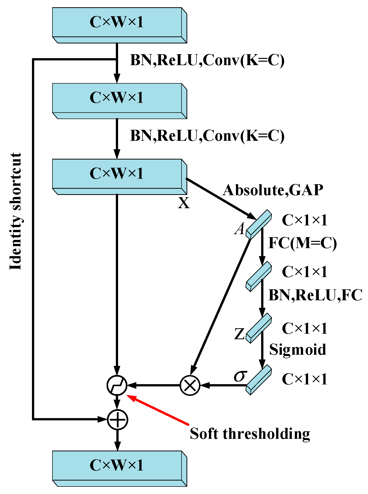
2.1. Deep Residual Shrinkage Network

DRSN is an improved network based on the deep residual network [27]. The principle of DRSN is to focus on the important features that are beneficial to the current task through the attention mechanism, while the non-important features are set to zero through the soft threshold function [28], so as to enhance the ability of the deep neural network to extract useful features from noisy signals.

DRSN can be divided into two types, which are the channel-shared threshold (CS) and the channel-wise thresholds (CW). Each channel shares a threshold in the CS type and has an independent threshold in the CW type. Generally speaking, the noise information contained in the feature map of each channel is different. Each channel has an independent channel threshold that can process noise information more flexibly and obtain a higher classification accuracy. At the same time, [28] confirmed that the calculation time of DRSN-CW is shorter than that of DRSN-CS. Therefore, the CW were adopted in this study.

DRSN includes a soft threshold and attention mechanism. The input data whose absolute value is less than the threshold value can be set to 0 by the soft threshold and shrink the input data whose absolute value is greater than the threshold value toward zero. At the same time, soft threshold can also reduce the risks of gradient dispersion and gradient explosion that deep learning algorithms can encounter to a certain extent [29]. However, there is an obvious shortcoming when soft threshold is applied alone. That is, it cannot adaptively adjust the size of the threshold according to the different characteristics of the noise of each sample.

The attention mechanism can be simply comprehended as focusing on the target object after quickly scanning the global information and ignoring the non-target information, finally suppressing the interference of irrelevant information while extracting more detailed information of the target object. Squeeze and excitation network (SENet) adopts one small sub-network to obtain a set of weights, and then multiplies this set of weights with the features of each channel to adjust the size of each channel feature [30].

The DRSN uses the aforementioned SENet unit for reference, and the residual shrinkage building unit with channel-wise thresholds (RSBU-CW) shown in Figure 2 is applied to achieve a soft threshold under the deep attention mechanism. In the RSBU-CW unit, K is the number of convolutional kernels in the convolutional layer, M is the number of neurons in the fully connected layer (FC), C, W, and 1 in C × W × 1 are the indicators of the number of channels, width, and height of the feature map, respectively.

In the RSBU-CW unit, a new feature $A$ is obtained through absolute value and global average pooling from a feature X. In another path, feature $A$ first passes through a small fully connected network, and finally normalizes the output to between 0 and 1 through the Sigmoid function to obtain the coefficient $\sigma$. Therefore, the threshold value $\tau$ after the soft threshold can be expressed as $A$ × $\sigma$. The calculation formula of the Sigmoid function is shown as:

$${\sigma }_n=\frac{1}{1+{\mathrm{e}}^{-z_n}}$$

(1)

where $z_n$ is the feature at the n-th neuron, and ${\sigma }_n$ is the n-th scaling parameter. After that, the thresholds are calculated by

$${\tau }_n={\sigma }_n\cdot \underset{i,j}{globalaverage}\left|x_{i,j,n}\right|$$

(2)

where ${\tau }_n$ is the threshold for the n-th channel of the feature map and i, j, n are the indexes of width, height, and channel of the feature map X, respectively.

The construction of the RSBU-CW unit ensures that the thresholds of different samples are different. Therefore, the RSBU-CW unit can be understood as another manifestation of the attention mechanism: through soft thresholding, features irrelevant to the current task are set to 0, while those relevant to the current task are retained.

Structurally, the DRSN consists of a convolutional layer, activation layer, global average pooling layer (GAP), batch normalization (BN), a certain number of RSBU-CW units, and several fully connected layers.

However, since DRSN does not contain recurrent neurons in its structure, it is not easy for DRSN to capture the characteristics of correlation and dependence between data when faced with long sequences of data. In short, compared with the dynamic time series feature mining model, the structure of DRSN determines that it is more sensitive to the static features contained in the sample.

2.2. Improved Deep Residual Shrinkage Network

In order to address the defect of DRSN, an improved structure of DRSN is proposed. An LSTM branch is added to the DRSN to compensate for the dynamic timing characteristics required by the diagnostic network. At the same time, replacing the ReLU activation function used in DRSN with the Mish function can better allow information to penetrate into the neural network and thus improve the accuracy of network classification.

LSTM is one of the variants of the recurrent neural network (RNN) [31]. The architecture of LSTM is shown in Figure 3, and its principle can be expressed as follows: the discarded information is determined through the forgetting gate, the information of the previous hidden state and the information of the current input are transmitted through the input gate, and the value of the next hidden state is determined through the output gate.

Mish is a self-regularized non-monotonic neural activation function [32]. It can be expressed as:

$$\mathrm{Mish}(x)=x\cdot \tanh (\log (1+{\mathrm{e}}^x))$$

(3)

Mish has the advantage of being a non-monotonic function, which helps the network maintain a small negative value in the calculation process and thus stabilize the gradient flow of the network. In addition, it has infinite order continuity and smoothness, which makes it an efficient way to optimize the output and improve its quality.

Deep neural network (DNN) is a variety of neural network with at least one hidden layer, which can provide modeling for complex nonlinear systems. Compared with the shallow neural network, the additional hidden layer of DNN provides a higher level of abstraction for the model and improves the capability of the model.

Through the above analysis, an end-to-end fault diagnosis model based on improved DRSN is proposed. The complete structure of the proposed network is shown in Figure 4, which is mainly composed of DRSN, LSTM, and DNN. In the network, Conv2D represents the two-dimensional convolution layer. “/2” means to move the convolutional kernel with a stride of two to reduce the width of the output feature map. First of all, the improved network reduces the impact of noise on the network and extracts the static characteristics of the fault samples by the DRSN branch. Furthermore, it memorizes and mines the dynamic timing law of the fault samples in the time dimension by the LSTM branch. Then, the network connects the fault features of the output of the two branches in series and uses DNN to further mine them. DNN can re-code the combined features to remove some redundant information contained in the features and help the model to accomplish the target task better. Finally, the output of DNN was classified by Softmax funtion.

2.3. Process of PV Fault Diagnosis

A PV fault diagnostic method based on improved DRSN is proposed, and its execution process is as follows:

(1)

Solar system analyzer is used to collect the I-V curves of the PV array.

(2)

Adopt the open-circuit voltage and short-circuit current at the STC of the array to standardization the voltage and current data, and reconstruct the standardized voltage and current into an n × 2 matrix as the input of the diagnostic model.

(3)

The samples are randomly divided into three categories by proportion including training set, validation set, and test set.

(4)

Input the training set samples into the improved DRSN model. The model adaptively learns the characteristics of the training set samples and uses the validation set samples to adjust the network weights until the accuracy of the model validation set converges.

(5)

Input the test-set samples into the trained model to evaluate the fault diagnosis performance of this model.

3. Experimental Verification

3.1. Introduction to the Experimental Platform

A PV experimental field with a capacity of 6.48 kWp, called field A, was established to evaluate the performance of the proposed method. There are 24 PV modules in it, including two series and 12 PV modules in each series. The parameters of each PV module are illustrated in

Table 1. The parameters of the PV module in field A under STC.

Pm	Vm	Im	Voc	Isc
270 W	31.3 V	8.63 A	38.5 V	9.09 A

. In this study, the fault diagnosis of the single-string PV system is analyzed first. The simulation of the fault is shown in Figure 5. The model of the solar system analyzer is PROVA1011(TES Electrical Electronic Corp, Taiwan, China), which was used to collect the I-V curves of the PV system. Meanwhile, two Y-shaped taps are short-connected to simulate SC faults. Due to its good shading properties and because it is not easily deteriorated when exposed to the sun, corrugated cardboard is chosen to shelter the PV array to simulate PS-BO fault. At this moment, the bypass-diode of the sheltered PV module is turned on. PS-BR faults are simulated by plastic bags with a higher light transmittance, and the bypass-diode of the sheltered PV module reverses. A sliding rheostat is connected in series in the module to simulate the Aa fault of the module. The irradiance range of all experimental samples is about 150 to 1000 W/m².

The sample category and number of samples are found in

Table 2. Summary of measured experimental fault type.

Fault Type Description	Category Label	Sample Number
Normal	Class 0	200
SC	Class 1	200
PS-BR	Class 2	200
PS-BO	Class3	200
Aa	Class 4	200
SC & PS-BO	Class 5	200
SC & PS-BR	Class 6	200
SC & Aa	Class 7	200
PS-BO & Aa	Class 8	200
PS-BR & Aa	Class 9	200
PS-BR & PS-BO	Class 10	200

, including the single-fault and hybrid-fault category. The data of four single faults including SC, PS-BO, PS-BR, and Aa, and six hybrid faults composed of two arbitrary single-fault combinations, such as SC and PS-BO representing the combination of SC and PS-BO faults. The data are randomly selected by different sample categories at a proportion of 6:2:2, and a total of 1320 sets of data are adopted as the training set, and the sets of the validation and the test set are both 440.

The application of traditional PV fault diagnostic methods usually faces the severe challenges of remote data transmission and cloud storage, which, fortunately, has been effectively solved by edge computing. Therefore, the designed diagnostic model needs to be lightweight enough to run efficiently on equipment with limited computing power. In this study, the algorithm is directly trained and tested on Raspberry Pi 4B, the operating system is Ubuntu 21.04, and the software platform is Keras.

3.2. Selection of Hyper-Parameters

After repeated parameter tuning, the hyper-parameters of the model are depicted in

Table 3. Parameters used in experimental verification.

Layer Type	Kernel Size	No. of Kernel	Stride	Activation	Output
Input layer	-	-	-	-	149 × 2 × 1
Conv2D	(3, 3)	8	(1, 1)	-	149 × 2 × 8
Residual	number of RSBU-CW units = 6 out_channels = 8 downsample_strides = 2				3 × 1 × 8
shrinkage
block
LSTM	output dimension = 16, dropout coefficient = 0.2				16
Dense1	num_neurons = 256			ReLU	256
Dense2	num_neurons = 128			ReLU	128
Dense3	num_neurons = 64			ReLU	64
Output layer	11	1	-	Softmax	11

. Table 3 defines the layer names based on Figure 4. Specifically, the residual shrinkage block consists of six RSBU-CW units, and the hyper-parameter setting in each unit is kept consistent. The Mish function of each activation layer in the RSBU-CW unit is investigated. The number of channels for the output feature map is set to eight and the downsample strides is set to two. The output dimension of the LSTM layer is set to 16. To prevent network overfitting, the LSTM layer applies the dropout whose coefficient is set to 0.2. DNN consists of three Dense layers named Dense1, Dense2, and Dense3. Num_neurons represent the number of neurons in the Dense layer. The regularization method of the output layer is L2 regularization, and the regularization coefficient is set to 0.0015. The cross-entropy is selected as the loss function. In addition, during training, the maximum epochs of the network are 1000, the initial learning rate of Adam is 1 × 10⁻⁴, and the batch is equal to 32.

3.3. Feature Visualization

t-SNE (t-distributed stochastic neighbor embedding) is a machine learning algorithm suitable for reduction dimension, which was proposed by Maaten and Hinton in 2008 [33]. Moreover, t-SNE is a non-linear dimension reduction algorithm, which is fit for reducing the dimensionality of high-dimensional data to two or three dimensions to perform feature visualization. In this study, the PCA algorithm is adopted as a dimension reduction tool. Figure 6 shows the two-dimensional visualization results of t-SNE of the training set data, before and after model training. It should be noted that abscissa and ordinate in Figure 6 represent the corresponding locations where the samples map to low-dimensional space, which has no units.

The distribution of the original data is shown in Figure 6a. It can be found that most of the data are relatively discrete, randomly appearing in various regions. Only a small part of the data is relatively centralized. This phenomenon is caused by the fact that t-SNE is essentially a clustering algorithm with classification function. The sample features of normal, SC, PS-BR, and other types of data have not been mined before training, and the differences among samples are small, so it is difficult for the algorithm to cluster them. The I-V curves of PS-BO, SC and PS-BO, and PS-BO and Aa have serious distortion and obvious fault characteristics, so they have significant distribution intervals when they are inputted. However, the samples of these fault types still cannot be gathered in their respective characteristic intervals.

The feature visualization results of the output layer are shown in Figure 6b. At this time, the best discrimination between various types of data is achieved, and only a few samples of normal and Aa have obvious overlapping phenomenon. The reasons for this phenomenon are: (1) the sampling method of the solar system analyzer investigated in the experiment is non-uniform, and the data near the short-circuit point is denser, while the data near the open-circuit point is looser, which is the reason that the slope change near the open-circuit point is not obvious; (2) when Aa occurs in a PV module under low irradiance, the fault features of the sample are not obvious enough, and it is easy to be misjudged as a normal sample, which is also one of the difficulties of PV detection. Part of the Aa samples was collected under 500 W/m², and the I-V curves of these samples were close to the shape of normal samples, which resulted in the model not being able to correctly classify them.

3.4. Analysis of Model Training and Test Results

The changes in the accuracy and loss of the training set after 2000 iterations of the model are illustrated in Figure 7. The final training accuracy of the model reached 97.65%. The accuracy and loss of the training set quickly converge after 500 iterations. Thus, in order to speed up the training speed of the model, the final Epochs is set to 1000.

Accuracy, precision, and recall are commonly used evaluation indexes in the field of machine learning. The accuracy reflects the proportion of samples that are correctly identified. The recall reflects the recall ability of the algorithm; that is, the number of positive samples that are predicted correctly. The precision refers to the number of real positive samples among the samples whose predictions are positive. The calculation formula is as follows [34]:

$$\mathrm{Accuracy}=\frac{TP+TN}{TP+FN+FP+TN}$$

(4)

$$\mathrm{Recall}=\frac{TP}{TP+FN}$$

(5)

$$\mathrm{Precision}=\frac{TP}{TP+FP}$$

(6)

where TP is the true positive category, FN is the false negative category, FP is the false positive category, and TN is the true negative category.

The network weight with the optimal training accuracy is saved to generate a fault diagnosis model. The model is used to diagnose 440 test samples obtained from the experimental platform. A total of 430 samples are correctly identified, and the overall accuracy is 97.73%. It is worth noting that once the model weight parameters are fixed, the results are the same for the same test data or test set. In order to make the performance of the model to be reflected more intuitively on the test set, a confusion matrix is used to display the classification results of the model. The results of the confusion matrix normalized row by row are shown in Figure 8a, which represents the index of recall, and the results of the confusion matrix normalized by the column are shown in Figure 8b, representing the index of precision. The labels of the samples in Figure 8 are consistent with Table 2. In Figure 8, the accuracy rate is represented in blue and the error rate is represented in red.

In Figure 8a, it is clear that 3% of the normal samples are judged as Aa ones. The recall of Aa samples was 0.80, and parts of samples were judged to be normal samples and PS-BR samples. The reason is that for these Aa samples judged as normal types, the slope change feature of I-V curve near the open point is not obvious enough, which leads to the model being not able to correctly identify them. The Aa samples judged to be PS-BR may be sheltered by dark clouds when measured and the double-peak feature of PS samples appeared on their I-V curve, which causes interference to the model diagnosis. In addition, a small number of PS-BR and Aa samples were misjudged as Aa samples. Except for the three types of samples, the recall rate of the other types of samples reached 100%.

It is observed from Figure 8b that aiming at the sample labels predicted by the model, except for the normal, PS-BR, and Aa samples, the prediction results of the other types of samples are both completely correct.

3.5. Influence of Different Irradiance

In order to test the identification accuracy of the proposed method under different irradiance, the collected 440 test-set samples were divided into high irradiance (800 W/m² ≤ G ≤ 1000 W/m²), medium irradiance (500 W/m² < G < 800W/m²), and low irradiance (150 W/m² ≤ G ≤ 500 W/m²), respectively. The test results are shown in

Table 4. Test result in different irradiance.

Fault Type	Testing Accuracy
	150–500 W/m2	500–800 W/m2	800–1000 W/m2	Total Accuracy
Normal	90%	100%	100%	97.5%
SC	100%	100%	100%	100%
PS-BR	100%	100%	100%	100%
PS-BO	100%	100%	100%	100%
Aa	50%	88.9%	100%	80%
SC & PS-BO	100%	100%	100%	100%
SC & PS-BR	100%	100%	100%	100%
SC & Aa	100%	100%	100%	100%
PS-BO & Aa	100%	100%	100%	100%
PS-BR & Aa	100%	95.2%	100%	97.5%
PS-BR & PS-BO	100%	100%	100%	100%
Total	93.2%	98.5%	100%	97.73%

. It is clear that the accuracy of proposed method has a certain difference under different irradiance. The diagnostic accuracy under high irradiance reaches 100%, but under low irradiance the accuracy is only 93.2%. Compared with the condition of high irradiance, the diagnostic accuracy dropped by 6.8% in the low irradiance. Although the accuracy of the diagnosis model is low under low irradiance, the misjudged samples mainly appear on the Aa samples, and the model can still maintain a high accuracy of other types of samples. The reason is that, in the case of low irradiance, the I-V curve of the PV array tends to be distorted to a certain extent, resulting in the inconspicuous fault characteristics of the sample, which is consistent with the analysis results in Section 3.3.

3.6. Verification in a Multi-String System

In order to further evaluate the applicability of the diagnostic network in the multi-string PV system, a double-string experiment was also carried out in this study. It can be seen from Table 1 that the short-circuit current of single-string PV modules under the STC condition is 9.09A, and the short-circuit current of double-string modules in parallel are much higher than 12A. However, the maximum current range of the solar system analyzer (PROVA1011) used in the research is only 12A, so experiments were carried out under low irradiance. During the experiment, the irradiance was kept below 600 W/m² to obtain the I-V curve.

The data of normal, SC, and PS-BO were collected in the experiment, and the sample numbers of each type were 106, 125, and 116, respectively. The data samples were randomly divided according to the ratio of 6:2:2. The hyper-parameters setting of the model are consistent with that of the single-string experiment. Finally, the trained model was developed to classify faults in the test set. Table 4 shows the test results, using recall as the evaluation index.

It can be seen from

Table 5. Test result of the double-string experiment.

Fault Type	Normal	SC	PS-BO
Sample number	21	25	23
Recall (%)	100%	100%	100%

that the model shows high identification accuracy for all three types of samples. The experimental results show that the diagnostic model is also suitable for multi-string PV arrays. In short, the diagnostic method can meet the requirements of the PV experimental field with different wiring types. When the scale of the PV array changes, the model needs to be retrained.

3.7. Analysis of Anti-Interference Ability

When performing I-V curve measurement, data collection is usually interfered by equipment noise. As the noise intensity increases, it inevitably causes interference to the fault diagnosis of the model and generates a decrease in the accuracy of the network. The adaptive ability of the model was evaluated by adding Gaussian white noise to the data.

The signal-to-noise ratio (SNR) reflects the ratio of the normal signal to the noise signal [35]. The larger the SNR, the smaller the noise mixed in the normal signal. The calculation formula is:

$$\mathrm{SNR}=20{\log }_{10}(\frac{1}{\epsilon })$$

(7)

where ε represents the percentage of noise.

In order to further analyze the advantages of the proposed method in terms of anti-interference ability, the convolutional neural network (CNN) model, and the deep residual network (ResNet) model proposed in [24] were constructed to compare with the proposed method. The CNN model adopts the traditional VGG-16 structure. The test results of the above several models under different SNRs are shown in

Table 6. Classification accuracy under different SNR.

ε (%)	SNR	Proposed Method	CNN	ResNet
0	-	97.73%	88.41%	93.18%
0.316%	50 dB	97.73%	88.41%	93.18%
1%	40 dB	97.73%	88.41%	93.18%
3.162%	30 dB	97.73%	87.05%	92.05%
10%	20 dB	94.09%	85.00%	91.36%
31.622%	10 dB	92.50%	77.50%	87.27%

.

The test results indicate that the anti-interference ability of the proposed method is the best among several models. The proposed method, which contains a soft threshold and attention mechanism, amplifies target information and ignores non-target information when extracting features from samples. The non-target information of the sample contains a certain amount of noise interference. After using the soft threshold, the proportion of target information in the remaining features increases significantly. In other words, the influence of noise on the model is significantly decreased by soft threshold. The increase of noise intensity has no obvious impact on the diagnostic results of the model, and the diagnostic accuracy does not decrease significantly until the noise intensity is greater than 10%. However, the noise intensity in practical engineering is generally maintained at a small amplitude. In other words, the proposed method is not disturbed by noise in practical applications.

4. Comparison and Discussion

4.1. Performance Evaluation of Improved DRSN

In order to further analyze and evaluate the improvement measures of the proposed method, the LSTM and DRSN models were constructed respectively. Then, the three models were tested with the same measurement data set and distribution proportion.

Table 7. Execution result of different models.

Model	Proposed Method	LSTM	DRSN
Training accuracy	97.65%	89.24%	95.15%
Testing accuracy	97.73%	87.05%	96.60%
Running time/epoch	6 s	5 s	1 s
Test time/sample	0.0318 s	0.0102 s	0.0360 s

shows the executing results of the three models. It can be clearly seen that the proposed model has a highest accuracy on both the training and test set, and the test time is less than the DRSN model. The test time of the LSTM model is the least, but the test accuracy is the lowest, which obviously indicates that the results from using a separate LSTM are limited. The diagnosis time of the DRSN model is the slowest; moreover, the extracted features are not complete, and the accuracy is lower than the proposed method.

4.2. Comparison and Analysis of Different Methods

Briefly, the proposed method integrates the advantages of LSTM and DRSN, which achieve a better classification effect in a shorter diagnosis time by the static features mined by DRSN and the dynamic timing law memorized by LSTM.

For further evaluation of the performance of the proposed method, a quantitative comparison was carried out between the proposed method and the other three methods used in [21,24,36], and the results are shown in

Table 8. Comparison of the test results of different methods.

Method	Proposed Method	[21]	[24]	[36]
Accuracy (%)	97.73	89.55	93.18	78.86
Test time (ms)/sample	31.8	27.9	26.2	10.7

and Figure 9. In order to ensure the fairness of the quantitative comparison, the same dataset and data partition method adopted in Section 3.1 were used to test the four methods. In other words, this study reproduces the methods proposed in [21,24,36] by Matlab or Python, and the dataset in Section 3.1 were used to evaluate the fault diagnosis performance of these methods.

Huang et al. [21] optimally solved the nonlinear least square method to standardize the external parameters of the PV system. Then, [21] applied the normalized external parameters as the characteristics, and the stage-wise additive modeling using multi-class exponential loss function based on the classification and regression tree (SAMME-CART) algorithm was investigated to realize the PV fault classification. In [24], Chen et al., adopted a non-uniform downsampling technique to process the data from the I-V curve, and then reconstructed the voltage, current, irradiance, and temperature into a 4 × 40-dimensional input matrix, and finally applied the residual neural network to classify the faults. Zaki et al. [36] first calculated the standardized maximum power point voltage V_m, the maximum power point current I_m, and the PV module fill factor FF as input data, and then joined CNN for fault classification to identify the single fault such as open circuit, shading, and line–line fault.

When building the model, the features used in [36] cannot deal with the single-fault and hybrid-fault mentioned in this study, so I_sc, V_oc, I_m, V_m, Temperature, Irradiance, FF, and R_oc (the slope of open-circuit point) are investigated as input fault characteristics. The construction of the ResNet model is consistent with the structure proposed in [24]. The test results show that the proposed method is significantly better than the other three methods, not only in terms of the overall accuracy of the test set, but also the recall and precision of a single category, and that the classification effect is best. Comparing the diagnosis time of a single sample, although the proposed method is the slowest and since the diagnosis time of several methods is so short, there is no significant difference in practical applications.

Compared with the two methods of extracting fault feature points in [21,36], the proposed method and [24] performed significantly better on the test set, which proves that the I-V curve is directly applied, as the input can retain more fault characteristic information. Despite this, using the I-V curve as an input can retain the timing characteristics of the curve, which is impossible for the other two methods. The overall accuracy of [24] is 93.18%, which is the best besides the method proposed in this study, but it does not perform very well in categories such as Normal, SC and PS-BR, and Aa, and many misjudgments occur.

Although the overall accuracy of [21] is not as good as [24], it also realizes the effective identification of most of the fault samples, and the performance is better when the types of samples are SC, PS-BO, SC and PS-BO, PS-BO and Aa, and PS-BR and PS-BO.

As for [36], even if the input is changed, the identification accuracy of this method is still the worst among all methods, and the identification accuracy of [21] with similar input is much better than [36]. That is due to the model in [36] only using a two-layer CNN structure whose simple shallow network leads to a poor network extraction of features, and the fault features cannot be effectively retained.

It can be seen from Figure 9 that the diagnostic accuracy of the Aa fault is much lower than that of other categories. The inability of the diagnostic model to fully distinguish normal samples from Aa samples is the main reason for this phenomenon, which can also be observed in Figure 6. In addition to the two points mentioned in Section 3.3, another reason for this phenomenon is that the aging resistance of some samples is not large enough, that is, only 6 $\mathrm{\Omega }$, which makes the slope change of the open-circuit point of I-V curve not obvious enough and increases the detection difficulty.

5. Edge Diagnosis of PV Faults

The traditional fault diagnosis process of PV module is shown in Figure 10. When troubleshooting the array, it is necessary to temporarily stop the grid connection, the solar system analyzer is used to extract the I-V curve of the array, and then copy the I-V curve to the computer for fault identification. The long-distance transmission of data and the decrease in energy utilization caused by the diagnosis process were the most serious defects of the traditional diagnostic method. In addition, another disadvantage of it is that the maintenance process is complex and requires on-site operation.

With the development of inverter technology, some commercial inverters can realize I-V curve scanning online, so the proposed algorithm can be embedded into the CPU of the inverter to realize fault diagnosis. In order to ensure that the diagnostic method can be applied to ordinary inverters, this study investigates a PV fault edge diagnosis system based on Raspberry Pi. The structure is shown in Figure 11. The device consists of two parts, Part I in Figure 11 is the control circuit. S1 is the control switch used to cut off the connection between the PV and inverter so as to complete the I-V curve scanning. MOSFET chooses the NVHL020N120SC1 module with a maximum drain-to-source voltage of 1200 V and a maximum saturation drain-source current of 103 A. Under the control of Raspberry Pi, the gradual change process from turn-off to turn-on is completed within 2 s; that is, the I-V curve scanning. Voltage and current are collected by selecting hall sensors. Part II in Figure 11 is the control core of the device, the control module is Raspberry Pi, and the AD sampling module is AD7606. When the fault diagnosis is needed, the command is first issued to control the MOSFET operation, and the voltage and current signals are collected by AD7606. Then, the fault diagnosis program is called to complete the PV status recognition. Finally, the diagnosis results are uploaded to the cloud. Operation and maintenance personnel can start fault diagnosis and view diagnosis results in real time through the mobile APP.

In order to verify whether Raspberry Pi meets the requirements of fault diagnosis, the same training set and validation set were used to train the diagnosis model in advance on PC and Raspberry Pi, and then the same software platform was applied to diagnose the same test-set samples. The hardware parameters of the PC are: XEON W-2123 CPU, 2 pieces of GTX1080Ti GPU, and 32 GB RAM. The model of Raspberry Pi is Raspberry Pi 4B, the operating system is Ubuntu 21.04, and the software platform is Keras. After testing, the diagnosis time of each sample on the PC is 0.0305 s, and the time of Raspberry Pi is 0.0318 s. The diagnosis time of the two devices is very close. Experiments show that it is reasonable to use Raspberry Pi as a lightweight diagnostic device.

The information interaction between the cloud and the edge terminal is a bidirectional process. With the aging of the array, the number of fault samples continues to increase, and the fault database will be gradually improved. Operation and maintenance personnel can send instructions to the Raspberry Pi in the cloud to fine tune the parameters of the model to maintain the accuracy of model diagnosis. At the same time, in order to reduce power consumption and maintain diagnostic accuracy, the diagnostic system can be set to start at noon every day. At this time, the light intensity reaches the maximum, and the interference caused by environmental factors to the diagnostic results is the minimum.

6. Conclusions

In this study, an improved deep residual shrinkage network fault diagnostic method is proposed by observing the I-V curve shape characteristics of a PV array under single- and hybrid-fault states. The proposed method consists of DRSN, LSTM, and DNN. The DRSN branch can reduce the impact of noise on the network and extract the static characteristics of fault samples, while the LSTM branch can remember and mine the long-term dependence and temporal correlation of fault samples in the dimension of time. Finally, DNN can recode the combined features of the two branches, remove some redundant information contained in the features, and improve the classification accuracy. The results show that the improved model can accurately identify single and hybrid faults, and the classification accuracy of test set reaches 97.73%, which verifies the effectiveness of the proposed method. At the same time, the method does not need to use environmental parameters such as temperature and irradiance, and can be applied to PV power plants even if they lack environmental sensors. In addition, a fault edge diagnosis scheme of PV array based on Raspberry Pi is proposed, which can meet the needs of fault diagnosis and has a high practical application potential.

References

1. Wang, Z.; Yang, G. Static operational impacts of residential solar PV plants on the medium voltage distribution grids—a case study based on the danish island bornholm. Energies 2019, 12, 1458. [Google Scholar] [CrossRef] [Green Version]
2. Agoua, X.G.; Girard, R.; Kariniotakis, G. Photovoltaic power forecasting: Assessment of the impact of multiple sources of spatio-temporal data on forecast accuracy. Energies 2021, 14, 1432. [Google Scholar] [CrossRef]
3. Renewables 2021 Global Status Report. Available online: https://www.ren21.net/reports/global-status-report/ (accessed on 15 December 2021).
4. Sun, X.; Chavali, R.V.K.; Alam, M.A. Real-time monitoring and diagnosis of photovoltaic system degradation only using maximum power point-the Suns-Vmp method. Prog. Photovolt. Res. Appl. 2019, 27, 55–66. [Google Scholar] [CrossRef] [Green Version]
5. Fadhel, S.; Delpha, C.; Diallo, D.; Bahri, I.; Migan, A.; Trabelsi, M.; Mimouni, M.F. PV shading fault detection and classification based on I-V curve using principal component analysis: Application to isolated PV system. Sol. Energy 2019, 179, 1–10. [Google Scholar] [CrossRef] [Green Version]
6. Dhimish, M.; Holmes, V.; Mehrdadi, B.; Dales, M. The impact of cracks on photovoltaic power performance. J. Sci. 2017, 2, 199–209. [Google Scholar] [CrossRef]
7. Abderrezek, M.; Fathi, M. Experimental study of the dust effect on photovoltaic panels’ energy yield. Sol. Energy 2017, 142, 308–320. [Google Scholar] [CrossRef]
8. Zhao, Y.; de Palma, J.-F.; Mosesian, J.; Lyons, R.; Lehman, B. Line-line fault analysis and protection challenges in solar photovoltaic arrays. IEEE Trans. Ind. Electron. 2013, 60, 3784–3795. [Google Scholar] [CrossRef]
9. Alam, M.K.; Khan, F.; Johnson, J.; Flicker, J. A comprehensive review of catastrophic faults in PV arrays: Types, detection, and mitigation techniques. IEEE J. Photovolt. 2015, 5, 982–997. [Google Scholar] [CrossRef]
10. Otamendi, U.; Martinez, I.; Quartulli, M.; Olaizola, I.G.; Viles, E.; Cambarau, W. Segmentation of cell-level anomalies in electroluminescence images of photovoltaic modules. Sol. Energy 2021, 220, 914–926. [Google Scholar] [CrossRef]
11. Parikh, H.; Buratti, Y.; Spataru, S.V.; Villebro, F.; Dos Reis Benatto, G.A.; Poulsen, P.B.; Wendlandt, S.; Kerekes, T.; Sera, D.; Hameiri, Z. Solar cell cracks and finger failure detection using statistical parameters of electroluminescence images and machine learning. Appl. Sci. 2020, 10, 8834. [Google Scholar] [CrossRef]
12. Cubukcu, M.; Akanalci, A. Real-time inspection and determination methods of faults on photovoltaic power systems by thermal imaging in Turkey. Renew. Energy 2020, 147, 1231–1238. [Google Scholar] [CrossRef]
13. Ali, M.U.; Khan, H.F.; Masud, M.; Kallu, K.D.; Zafar, A. A machine learning framework to identify the hotspot in photovoltaic module using infrared thermography. Sol. Energy 2020, 208, 643–651. [Google Scholar] [CrossRef]
14. Tsanakas, J.A.; Ha, L.D.; Shakarchi, F.A. Advanced inspection of photovoltaic installations by aerial triangulation and terrestrial georeferencing of thermal/visual imagery. Renew. Energy 2017, 102, 224–233. [Google Scholar] [CrossRef]
15. Hashemi, B.; Taheri, S.; Cretu, A.M.; Pouresmaeil, E. Systematic photovoltaic system power losses calculation and modeling using computational intelligence techniques. Appl. Energy 2021, 284, 116396. [Google Scholar] [CrossRef]
16. Xie, X.; Meng, F.; Luo, X.; Cai, S.; Ma, X.; Na, Z.; Ma, D.; Shan, Y.; Ge, L.; Liu, Y. Fault diagnosis and detection based on efficiency loss test of photovoltaic power station. In Proceedings of the 2020 6th International Conference on Energy Materials and Environment Engineering, Tianjin, China, 24–26 April 2020. [Google Scholar]
17. Dhimish, M.; Badran, G. Photovoltaic hot-spots fault detection algorithm using fuzzy systems. IEEE Trans. Device Mater. Reliab. 2019, 19, 671–679. [Google Scholar] [CrossRef] [Green Version]
18. Kuo, C.L.; Chen, J.L.; Chen, S.J.; Kao, C.C.; Yau, H.T.; Lin, C.H. Photovoltaic energy conversion system fault detection using fractional-order color relation classifier in microdistribution systems. IEEE Trans. Smart Grid 2017, 8, 1163–1172. [Google Scholar] [CrossRef]
19. Miao, W.; Lam, K.H.; Pong, P.W.T. A string-current behavior and current sensing based technique for line-line fault detection in photovoltaic systems. IEEE Trans. Magn. 2017, 57, 1–6. [Google Scholar] [CrossRef]
20. Lu, X.; Lin, P.; Cheng, S.; Lin, Y.; Chen, Z.; Wu, L.; Zheng, Q. Fault diagnosis for photovoltaic array based on convolutional neural network and electrical time series graph. Energy Conv. Manag. 2019, 196, 950–965. [Google Scholar] [CrossRef]
21. Huang, J.M.; Wai, R.J.; Gao, W. Newly-designed fault diagnostic method for solar photovoltaic generation system based on IV-curve measurement. IEEE Access 2019, 7, 70919–70932. [Google Scholar] [CrossRef]
22. Gao, W.; Wai, R.J. A novel fault identification method for photovoltaic array via convolutional neural network and residual gated recurrent unit. IEEE Access 2020, 8, 159493–159510. [Google Scholar] [CrossRef]
23. Chine, W.; Mellit, A.; Lughi, V.; Malek, A.; Sulligoi, G.; Pavan, A.M. A novel fault diagnosis technique for photovoltaic systems based on artificial neural networks. Renew. Energy 2016, 90, 501–512. [Google Scholar] [CrossRef]
24. Chen, Z.; Chen, Y.; Wu, L.; Cheng, S.; Lin, P. Deep residual network based fault detection and diagnosis of photovoltaic arrays using current-voltage curves and ambient conditions. Energy Conv. Manag. 2019, 198, 111793. [Google Scholar] [CrossRef]
25. Aziz, F.; Haq, A.U.; Ahmad, S.; Mahmoud, Y.; Jalal, M.; Ali, U. A novel convolutional neural network based approach for fault classification in photovoltaic arrays. IEEE Access 2020, 8, 41889–41904. [Google Scholar] [CrossRef]
26. Chen, S.Q.; Yang, G.J.; Gao, W.; Guo, M.F. Photovoltaic fault diagnosis via semisupervised ladder network with string voltage and current measures. IEEE J. Photovolt. 2021, 11, 219–231. [Google Scholar] [CrossRef]
27. Yang, J.; Gao, T.; Jiang, S.; Li, S.; Tang, Q. Fault diagnosis of rotating machinery based on one-dimensional deep residual shrinkage network with a wide convolution layer. Shock Vib. 2020, 2020, 8880960. [Google Scholar] [CrossRef]
28. Zhao, M.; Zhong, S.; Fu, X.; Tang, B.; Pecht, M. Deep residual shrinkage networks for fault diagnosis. IEEE Trans. Ind. Inform. 2020, 16, 4681–4690. [Google Scholar] [CrossRef]
29. Chen, G.; Lu, J.; Yang, M.; Zhou, J. Learning recurrent 3D attention for video-based person re-identification. IEEE Trans. Image Process. 2020, 29, 6963–6976. [Google Scholar] [CrossRef]
30. Hu, J.; Shen, L.; Albanie, S.; Sun, G.; Wu, E. Squeeze-and-excitation networks. IEEE Trans. Pattern Anal. Mach. Intell. 2020, 42, 2011–2023. [Google Scholar] [CrossRef] [Green Version]
31. Chung, J.; Gulcehre, C.; Cho, K.H.; Bengio, Y. Empirical evaluation of gated recurrent neural networks on sequence modeling. arXiv 2014, arXiv:1412.3555. [Google Scholar]
32. Misra, D. Mish: A self regularized non-monotonic neural activation function. arXiv 2019, arXiv:1908.08681. [Google Scholar]
33. Maaten, L.V.D.; Hinton, G. Visualizing data using t-SNE. J. Mach. Learn. Res. 2008, 9, 2579–2605. [Google Scholar]
34. Lei, Y.; Jia, F.; Lin, J.; Xing, S.; Ding, S.X. An intelligent fault diagnosis method using unsupervised feature learning towards mechanical big data. IEEE Trans. Ind. Electron. 2016, 63, 3137–3147. [Google Scholar] [CrossRef]
35. Zhao, Z.; Li, J.; Wang, L.; Wen, D.; Gao, K.Z. Signal-to-noise ratio improvement of MAMR on CoX/Pt media. IEEE Trans. Magn. 2015, 51, 11–14. [Google Scholar] [CrossRef]
36. Zaki, S.A.; Zhu, H.L.; Al Fakih, M.; Sayed, A.R.; Yao, J. Deep-learning-based method for faults classification of PV system. IET Renew. Power Gen. 2021, 15, 193–205. [Google Scholar] [CrossRef]
Figure 1. Characteristics of the I-V curve in different states under STC. (a) Single fault states; (b) Multiple-fault states.
Energies 15 03961 g001
Figure 2. Building unit entitled RSBU-CW.
Energies 15 03961 g002
Figure 3. Architecture of LSTM.
Energies 15 03961 g003
Figure 4. Complete structure of proposed network.
Energies 15 03961 g004
Figure 5. PV experimental field.
Energies 15 03961 g005
Figure 6. t-SNE visualization result of measured experiment. (a) Original data; (b) Output data.
Energies 15 03961 g006
Figure 7. Training results of 2000 iterations. (a) Curve of accuracy–epochs; (b) Curve of loss–epochs.
Energies 15 03961 g007
Figure 8. Confusion matrix of measured experiment. (a) Confusion matrix of recall; (b) Confusion matrix of precision.
Energies 15 03961 g008
Figure 9. Comparison results of each fault category by four methods. (a) Comparison results of recall; (b) Comparison results of precision.
Energies 15 03961 g009aEnergies 15 03961 g009b
Figure 10. Traditional fault diagnosis process.
Energies 15 03961 g010
Figure 11. Workflow of the edge diagnosis system.
Energies 15 03961 g011