Tax or Clean Technology? Measuring the True Effect on Carbon Emissions Mitigation for Sweden and Norway

Abstract

Studies of carbon emissions typically focus on price and tax effects or technology. We argue that the two are closely linked within an economy in disequilibrium. Our goals are twofold: (1) to examine the combined role of: low CO₂ technology, fuel taxes and CO₂ tax on taming CO₂ emissions and (2) to build a counterfactual analysis by capturing anything else that causes emissions to diverge from the trend such as renewable energy, energy laws and the state of the economy. The equilibrium correction model (EqCM) suggests that emissions have a long-term relationship with economic growth, fossil fuel use, taxes and clean power sources. Both oil and gas extraction and economic growth raise Norway’s emissions, offsetting the mitigating effect of taxes. Sweden´s carbon fuel tax elasticity is 20%, a value far above Norway´s elasticity, even though these carbon taxes were phased-in under a period of macroeconomic instability, weakening their effectiveness. The income elasticity of emissions is negative for Norway and positive for Sweden. Emission cuts require (a) de-growth, (b) a higher tax on transport fuels and (c) electrification of transport. The effects of tax, technology, economic growth and those for the pre- and post-carbon tax era differ strongly in the two nations.

1. Introduction

The literatures on the economic valuation of carbon emissions (CO₂) have rarely used a disequilibrium framework for econometric analysis to explain the role of tax and technology in carbon emission mitigation strategies.

The Swedish economy has recorded rising carbon dioxide (CO₂) emissions in the years 1960–1976, but then saw falling emissions in 1976–2015. The rapid decline in emissions continued into the 2010–2019 period. In contrast, Norway´s emissions have steadily grown since the 1960s and only fell in 1990–1995, before rising again in 2005–2010, since then emissions have fallen until 2019. To control this growth, both countries introduced a carbon tax (price) in the 1990s (Sweden 1991; Norway 1991), an event which occurred under macroeconomic instability (low economic growth in Sweden in the 1990s), a new energy technology policy (nuclear energy in Sweden in the early 1970s; hydropower in Norway) and a cap on emissions. To unravel the emission factors, this study assesses whether emissions, the economy, fuel (carbon) taxes and consumer behavior (fossil fuel use), as well as the technology and the policy regime (including that of energy efficiency standards and clean technology programmes), are cointegrated and, if so, if there is a long-term equilibrium in CO₂ emissions. In the paper, a comparison is made of Norway and Sweden in order to observe the extent to which a fossil-fuel-rich economy like the former is better able to mitigate emissions than a fossil-fuel-poor economy such as Sweden. Cointegration is defined as a long-term equilibrium in the economy. We use an equilibrium correction model (EqCM) to find the long-term equilibrium among these economic and policy (tax) factors. The EqCM is defined as one (a) which has a well-defined equilibrium, and (b) in which adjustment takes place towards that equilibrium [1].

An equilibrium is a state from which there is no tendency to change [1]. The EqCM estimates both the short-term (cycle) and the long-term trend (permanent) of CO₂ emissions, which are subject to many influences aside from price. The EqCM based on the cointegration method breaks macroeconomic time series (emissions, economic growth, prices, electricity use, oil use) into a secular component and a cyclical component. Since the cyclical component dissipates over time, any long-term movement is attributed to the secular component [2].

To achieve macroeconomic stability, a control is needed [3,4,5], such as a target, i.e., a desired value of real consumption associated with cutting emissions which, in turn, is achieved by adjusting an instrument (i.e., taxation, government expenditure, subsidies, fraction of low-CO₂ electricity,). Changes in emissions, emission levels and cumulative past errors all need to be included in the rule to stabilize the target variables [1]. Adjustment of the instrument effect (tax) can be carried out within the EqCM. In the paper, we propose a new analytical method to explain emissions, building on the work of References [6,7,8].

This cointegration system assesses the combined effect of taxes and the announcement effect of a tax, defined as “an action taken to reduce the environmental impact that is the target of the tax, between the time of the announcement of the tax and its implementation, when this action would not have been taken in the absence of the tax had it not been announced” [9]. A CO₂ tax is a form of explicit CO₂ pricing, directly linked to the level of CO₂ emissions. It is expressed as a value per tonne of CO₂ tonne equivalent (per T- CO₂e). Energy taxes work as implicit CO₂ taxes and thus determine CO₂ prices. Taxes on CO₂ and on energy have been either endogenous or exogenous to induce technical change. This is the only paper that (a) develops disequilibrium macroeconomic models of CO₂ abatement, spanning decades, for the cases of Sweden and Norway, and (b) examines efforts to decarbonise an entire national economy since the effects of the tax should be seen in relation to other policy measures [10].

Our study extends the literature on emission pathways by assuming that short-term CO₂ emission responses to economic growth, prices, energy technology and hydrocarbon extraction are distinguishable from long-term responses. Emission cuts result from a decline in fossil energy use, including petroleum, gasoline and cuts in electricity generated by fossil fuels. These are CO₂-intensive sources of energy that are often central to major economic sectors such as industry, transport and households.

Many studies on CO₂ emissions rely on ex-post evidence, making it difficult to attribute the decline in CO₂ emissions only to tax rises. There are a variety of factors that dynamic macroeconomic models incorporate, often based on large-scale Computable General Equilibrium (CGE) models [7] or on dynamic optimization and macroeconometric models [11]. In recent years, econometric and other quantitative analysis of CO₂ abatement has expanded, including [12] a study of the Finnish economy; [13,14] of the U.S.; [15] and a study of the Canadian economy. The authors of [7] also carried out a statistical study on Europe.

Taxes are levied on fossil fuels for industrial processes, on transport fuels, on household fuels and on the power sector. Evaluation studies on tax do not consider the mutual interactions between pre-existing fuel taxes and CO₂ tax and policy instruments such as the low CO₂ standards for industrial equipment, transport and households. These mechanisms, along with that of the ETS allowance price “the actual spot price of CO₂ emissions”, affect the CO₂ price. The CO₂ price is a factor in determining the volume of emissions, and this price is determined by the supply and demand of CO₂ emission allowances. Similarly, the level of energy tax is determined by the energy content for each fuel but not by the CO₂ content of fuels. There are three taxes that affect fossil fuel use and emissions: energy taxes on fuels, direct CO₂ taxes, and the CO₂ prices determined within the ETS. The sum of these three taxes can be seen as a surrogate for the real effective price of CO₂ and other externalities.

Evaluation of the true tax effect is further complicated by fuel efficiency standards (this lowers the CO₂ content of final fuel use) and other taxes such as the energy tax. Before the introduction of CO₂ taxes in the 1990s, significant theoretical and empirical work was developed [16,17,18]. The latter favours a carbon tax to a cap-and-trade system (ETS), since the climate change damage curve is flat. Cap-and-tax can provide CO₂ price stability, which facilitates investments in low-CO₂ technology.

Literature Review

In this section, we discuss the CO2 mitigation studies, as well as those on the environment and the economic growth nexus.

CO₂ mitigation models can be broadly classified into three categories: the first are models of dynamic optimisation [19], such as the Global 2100 model by the authors of [20] and the Poles model by the authors of [21]. The second are CGE models based on the concept of equilibrium in the market, with price and wage clearing to match supply and demand. Thirdly, there are macroeconometric simulations, such as that in this paper, which are estimated based on time series data (see also [7,22,23]). These models produce tax (price) and output effects. Recent advances in the approach have evolved from simple regression models to cointegration systems that capture disequilibrium.

Studies largely focus on changes in emissions, which result from changes in prices and in GDP. Studies on the environment and growth mostly rely on macroeconomic models with a static approach that ignores the dynamics of the macroeconomic system. Macroeconomic studies in the 1990s for energy planning in Norway and Sweden used the CGE framework [24], which assumes fixed prices and output and fixed substitution elasticities. These studies indicate that the costs of reducing emissions range from 169 to 700 US tonne-CO₂ (2000 USD prices) with GDP (welfare) losses ranging from a gain of 3.2 % to a loss of −1.3% of GDP (Ibid.). These methods focus on a single nation, but recent models use panel techniques based on data on many economies, such as as in Reference [25], or in Reference [11]. More recent models use evidence from interviews to determine whether the CO₂ price changes have induced cuts [26].

Studies can be further subdivided into (a) direct tax on CO₂ and (b) “Cap and Trade” for an emissions trading (ETS) scheme or “Cap and Tax”. A global CO2 tax is sometimes considered a necessary tool to control emissions [19], while other studies find that the effectiveness of the tax depends on how fast a consumer reacts to a price change [27]. In Norway´s case, the CO₂ tax effect was found to be modest [8], while for the Swedish case, taxes are a powerful tool in cutting emissions [28]. Further positive evidence suggests that the carbon tax elasticity of demand for gasoline is three times larger than its price elasticity [6]. Evidence at the company level has established that a carbon tax reduces the carbon intensity of production for the Swedish economy [29,30,31].

After examining a high number of ex-post studies on CO₂ taxes for Scandinavian cities [32], three problems can be seen to explain the tax effect: frequent changes in tax rates, tax exemptions and “the too many variables” problem.

Four further studies on various types of CO₂ taxes support the argument for their effectiveness. A large-scale study confirms that many CO₂ tax systems do cut emissions around the world [33] and it is claimed that direct carbon pricing is the cheapest policy measure. A second study on UK manufacturing covering the 1970–2014 period confirms the effects of the tax in cutting sector-based emissions [9]. A study of Danish firms in [34] found that the effects of the CO₂ tax, the energy tax and the energy efficiency agreement were effective in reducing energy use and emissions. Studies by the OECD [35] favour CO₂ taxes and argue that the technology-based mitigation efforts are more expensive than price-based measures (tax or ETS).

An alternative method to price CO₂ is through the “Cap and Trade” system, which determines CO₂ prices to meet CO2 emissions targets [36]. However, both the energy price (tax) and the level of CO₂ tax (prices) will range from sector to sector. A cap-and-trade study on CO₂ price effects within the EU concludes that “what is available indicates that CO₂ emissions were reduced by an amount that was probably between 50 and 100 million tonnes” in 2006 and 2007 [37]. At the microeconomic level, studies on CO₂ emissions’ mitigation use both dynamic panel models (e.g., Reference [38] and error correction models applied on CO₂ prices [39]) that reveal that emissions decline with those prices. In short, most studies agree on the success of the tax in cutting CO₂ emissions, but sector- and fuel-based evidence is lacking: The transport and household sectors face the largest level of CO₂ tax rates which defies the theory of carbon tax.

The above review shows that most studies support the use of CO₂ taxes; however, studies on Sweden found no effect of carbon pricing (tax) on investment in energy efficiency or carbon reduction [40,41]. This lack of effectiveness for the tax is explained by the fact that the tax does not cover all emissions (around 40% of total GHG emissions for Sweden) and covers more than 60% for Norway [42]. A recent study (Ibid.) reports that the aggregate CO₂ tax (implicit and explicit types) is too low, but it is increasingly used in many countries, with a total of 57 initiatives.

In addition to using CO₂ prices to cut CO₂ emissions, cuts can also result from a lower electricity demand and lower fuel prices, offsetting higher CO₂ prices as in Reference [43]. Another study [44] echoes the finding of Reference [43]: the financial crisis was the key factor in lowering CO₂ emissions rather than the effects of the ETS (or CO₂ prices), that is, the assumption is made that the financial crisis reduced the demand for electricity and oil products. It is entirely feasible that cuts in CO₂ emissions also occur under conditions of lower income growth, changes in fuel taxes, carbon tax and the ETS-based CO₂ prices for the Scandinavian economies under study.

In Section 2, we discuss the evolution of economy-wide CO₂ emissions and mitigation policy in the period of 1960–2018, the practice of pricing CO₂ for the two countries, the theory and methods and the key hypothesis underlying the modelling work. In Section 3, we present the EqCM model; in Section 4, we discuss the results of the time series analysis of the carbon tax. Section 5 concludes.

2. Materials and Methods

In the section, we describe the trends of CO₂ emissions for both countries and the estimation method.

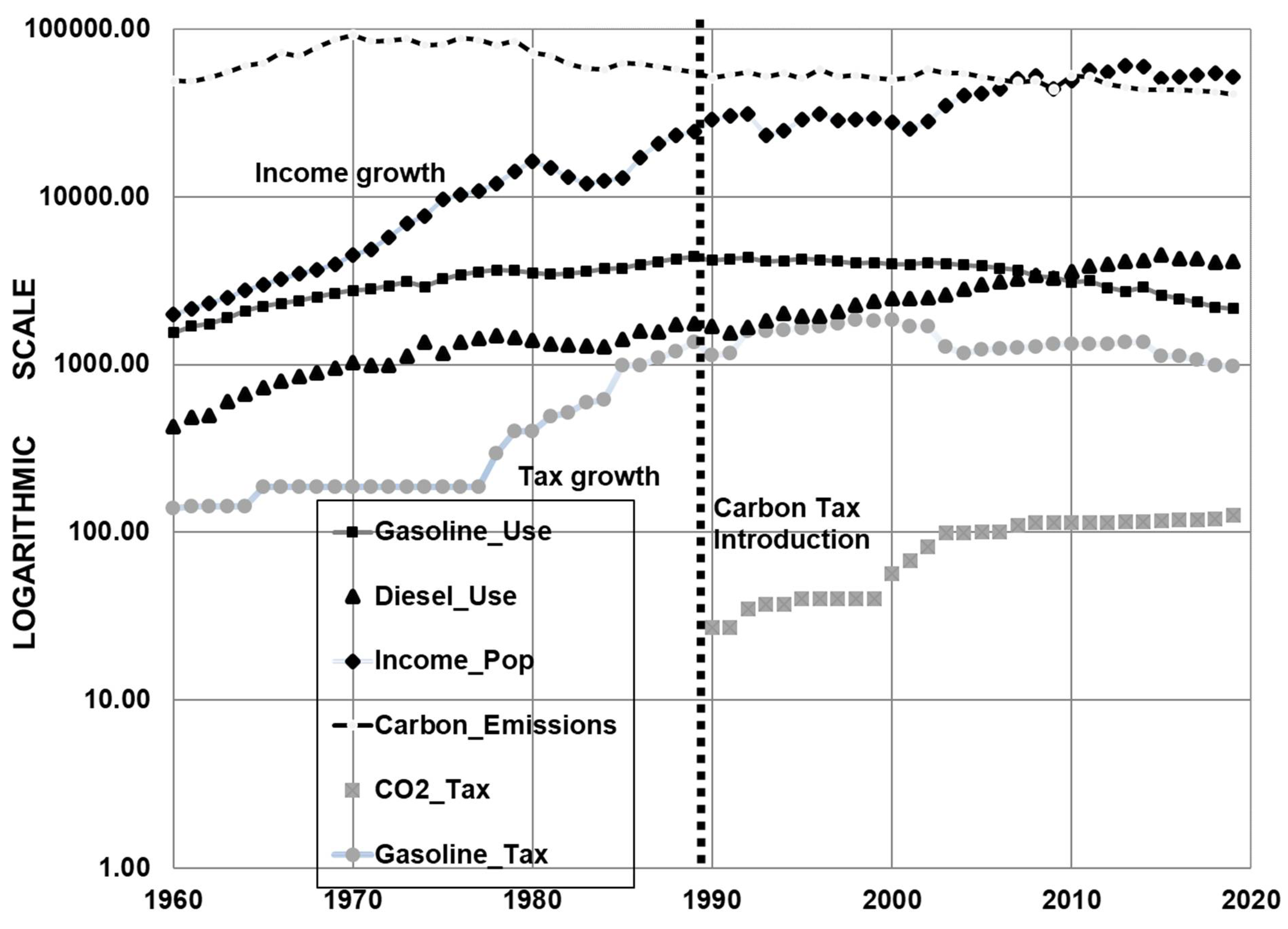
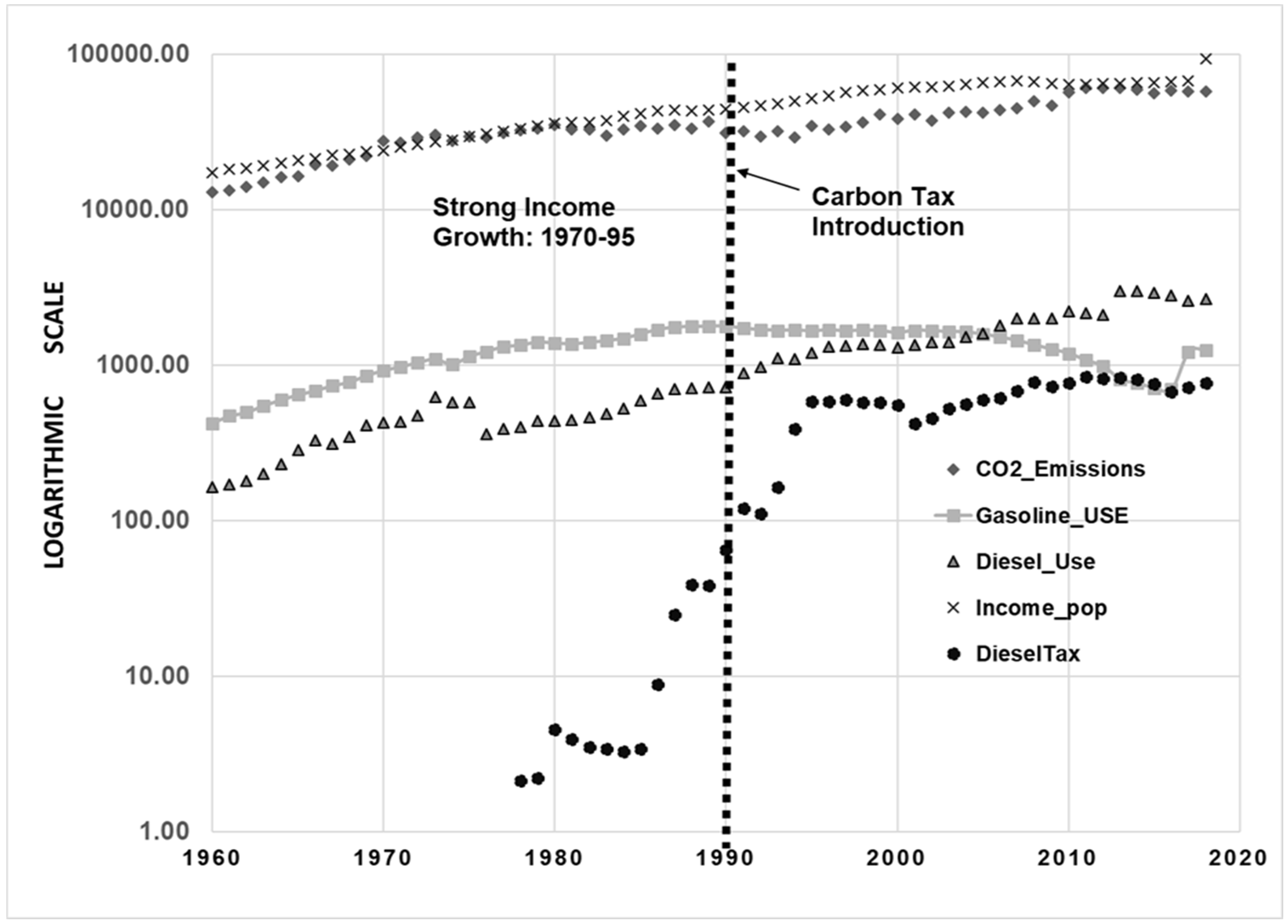
2.1. Materials: Trends Emissions of CO₂ of Sweden and Norway

In this section, a description of the data input is given for the macroeconomic relationships and the EqCM for the cases of Sweden and Norway for the years from 1960 to 2019. CO₂ emissions from the transport sector have not declined in Sweden and Norway, but some sectors have a seen a downwards shift in the growth path of CO₂ emissions as a result of (1) CO₂ tax, (2) the changes in energy mix within the industrial sectors, and (3) the diffusion of low-CO₂ electricity based on nuclear (in Sweden) and hydropower generation (in Norway). The energy systems of these two nations have recorded substantial fuel switching in the last 20 years, and this has supported CO₂ mitigation efforts. In contrast, the transport sector of both countries has recorded a steady growth in the CO₂ emissions path along with that of the household sector (Figure 1 and Figure 2), even though these sectors face the highest level of CO₂ tax rates. Diesel use continues to grow, despite higher fuel prices and taxes, while gasoline use is falling in both countries, with Sweden supporting biofuels and Norway supporting electric transport (Figure 1 and Figure 2).

Table 9 (Section 3.2) shows the list of all taxes currently levied in Sweden and Table 10 (Section 3.2) shows the climate policy decisions for transport and renewable energy sec-tors for Sweden: Green taxes in Sweden are overwhelmingly transport related; the Swe-dish government does not present a quantitative impact assessment of the effectiveness of those taxes.

Table 1. Annual changes in Sweden’s CO₂ emissions and changes in GDP: 1960–2019. Average annual growth rates in %. Source: [45,46,47,48,49].

Years	GDP (%/Year)	CO2 Emissions (%/Year)
1960–1965	5.18	4.94
1965–1970	4.05	8.08
1970–1975	2.59	−2.64
1975–1980	1.34	−2.35
1980–1985	1.99	−2.76
1985–1990	2.4	−3.9
1990–1995	0.71	−0.15
1995–2000	3.57	−0.38
2000–2005	2.62	0.7
2005–2010	1.59	0.37
2010–2019	1.31	−2.72

and

Table 2. Annual changes in Norway’s CO₂ emissions and changes in GDP: 1960–2019. Average annual growth rates in %. Source: Statistics Norway [47,48].

Year	GDP (%/year)	CO2 Emissions (%/Year)
1960–1965	4.63	4.6
1965–1970	3.75	11.29
1970–1975	4.84	1.15
1975–1980	4.53	3.38
1980–1985	3.33	−0.09
1985–1990	1.7	−2.1
1990–1995	3.73	2.16
1995–2000	3.68	2.14
2000–2005	2.2	1.8
2005–2010	0.76	6.15
2010–2019	2.86	−1.91

depict the change in Sweden’s and Norway´s CO₂ emissions. Swedish emissions in some years follow those in GDP, while, in the 1980s, CO₂ emissions were decoupled from GDP changes after the adoption of nuclear power. The noticeable change is that, for Sweden, the rate of improvement (lower emissions) declined after 1990–1995 until 2000. After 2000–2005, the rate of CO₂ emitted began to increase, but only slowly. In recent years, emissions have continued to decline whilst GDP continues to grow. We can detect a general decoupling of CO₂ emissions from GDP.

Table 11 (Section 3) tabulates the list of green taxes and the dates on which these were introduced in Norway. The oldest green tax was introduced in 1917 (annual tax on motor usage) and the newest in 2016 (road usage tax levied on LPG). As in Sweden, Norway´s taxes are dominated by the transport sector via petroleum fuels.

Norway’s emissions first grew in tandem with the growth in GDP in the early 1960s, then grew much faster than GDP to the end of that decade, but were far bw GDP growth in the 1970s and 1980s until this reversed again in the 1990s. Early in the century, emissions grew at a significantly higher level than GDP growth but they declined in recent years, although GDP growth is strong. The decoupling of CO₂ emissions from GDP is not as strong in Norway as it has been in Sweden. (Table 2).

Figure 1 (Sweden) and Figure 2 (Norway) describe how macroeconomic variables changed after the adoption of the CO₂ tax in Sweden 1990 and in Norway in 1991. The changes in magnitude of the variables of interest are also shown (Figure 1). The scale was adjusted to make magnitude changes comparable. Each major increment increases by a factor of 10.

Figure 1. CO₂ emissions and other energy-use indicators: Sweden 1960–2019. Source: IEA [49] & UN data [47], World Bank (2020) [46].

Figure 1. CO₂ emissions and other energy-use indicators: Sweden 1960–2019. Source: IEA [49] & UN data [47], World Bank (2020) [46].

Figure 2. CO₂ emissions, income and taxes: Norway 1960–2019. Source: (various years), [47,48,49].

Figure 2. CO₂ emissions, income and taxes: Norway 1960–2019. Source: (various years), [47,48,49].

How much an energy (CO₂) tax can be raised will depend on the oil price level, personal income, inflation, the social cost of carbon or the business cycle. For example, the upward change in taxes (CO₂ and energy) follows the economic cycle: periods of recession (lower output relative to trend) are associated with higher taxes and tax reductions track periods of economic expansion (Figure 1). For Sweden, GDP does not pull up the CO₂ emissions trend post-1990, although GDP does pull up the changes in diesel use through time. GDP again pulls up the tax on gasoline; this is an indication that they are cointegrated. Emissions are pulled up by gasoline use and diesel use, while CO₂ prices (using gasoline cost data) are pulled up by emissions in our sample. In short, these variables are cointegrated.

Unlike Sweden, Norway exports oil and gas, which has led to three effects: it pulls up GDP, and increases both emissions and personal income growth. The data also reveal that the CO₂ price (using diesel cost data) is stable for recent years, but its changes do track income growth (Figure 2). Prior to the CO₂ tax, emissions grew by 1.69 times in Sweden and 1.85 times in Norway, while, after the tax, emissions grew 0.83 and 0.86 times, respectively. The statistical evidence is stacked in favour of emissions being cut with a tax. Overall, there is a cointegration relationship between the emissions, GDP and fossil fuel use (diesel, petrol, household fuels) through time.

2.2. Key Relationships and Variables

This Section discusses (1) our hypothesis regarding the strongest effects on CO₂ emissions; (2) the description of the variables; (3) the model specification and 4) the error correction model.

2.2.1. Hypothesis of Equilibrium Relationships

The testing procedure is split into two areas. Firstly, we tested for unit roots for each of the variables to determine whether these were nonstationary (see Tables 7 and 8). Secondly, we tested whether the linear combinations of the variables were nonstationary or not. We proposed three hypotheses: (1) nuclear generation, hydropower for Norway and energy taxes for transport fuels both prompt rapid cuts in CO₂ emissions; (2) both fossil fuel use (mainly transport energy) and economic growth (measured by personal income before tax) are a cause of emissions for both countries; (3) a downward effect on emissions holds after the announcement effect and the adoption of the CO₂ tax. This is represented by the permanent effect dummy for the CO₂ tax policy. Hypothesis 1 is tested in Equation (1), Hypothesis 2 and 3 in Equations (1) and (4), while Hypothesis 3 is tested in Equations (1) and (4).

2.2.2. Data and Descriptive Statistics

For our analysis of CO₂ emissions, we defined the variables and present a data summary (

Table 3. Definition of variables for Sweden in sample.

Variable (Sweden)	Definition
Income per population	000′s; Constant 2010 USD.
CO2 Emissions	000′s Tonnes of CO2 equivalent per year
Diesel use	000′s Tonnes of fuel
Gasoline use	000′s Tonnes of fuel
Nuclear electricity generation	GWh
Trend	1960–2018
Gasoline taxes (implicit CO2 tax)	2014 Swedish Kronas per Tonne of fuel
Motor diesel Tax (implicit CO2 tax)	2014 Swedish Kronas per Tonne of fuel
CO2 tax (direct tax)	2014 Euro per Tonne of CO2

and

Table 4. Definition of variables for Norway in sample.

Variable (Norway: 1960–2018; Except Otherwise Indicated)	Definition
Income per population	000′s, constant 2005 USD.
CO2 Eq. Emissions (GHG)	000′s tonnes of CO2 equivalent per year
Oil and gas extraction: Value added (1971–2018)	Million Krones, 2018
Fossil fuel energy use (coal, oil, petroleum, natural gas)	% of total energy supply
Diesel use (transport)	000′s Tonnes of fuel
Gasoline use	000′s Tonnes of fuel
Hydro power	GWh
Trend (1960–2018)
Diesel taxes (1978–2018)	2014 Norwegian Krones per Tonne of fuel

). Annual data on CO₂ emissions or GHG emissions are taken from [45] and [46]. The rest of the data series were taken from [45]: population, gasoline and diesel consumption by the transport sector, and nuclear electricity generation. Data for gasoline taxes (implicit CO₂ tax), motor diesel tax (implicit CO₂ tax), and CO₂ tax are found in Reference [50]. Data on annual GDP were taken from Reference [46].

Annual data on CO₂ emissions, GDP, and population were taken from Statistics Norway (2020). Data on diesel tax, and value added by oil and gas extraction, were from the same source and data on fossil fuel shares were from the World Bank [46]. Data on diesel use and hydropower generation were taken from Reference [48].

2.3. Estimation Procedure

We transformed the series into their natural logarithms to reduce their variability and obtain the long-term elasticity values of emissions and CO₂ taxes. Short-term elasticities were obtained in the first-differences models that we explain below (Equations (1)–(6)).

Data transformations for the variables are explained in Equation (1). By taking the first differences in non-stationary variables, we can achieve the stationary relationships of Equation (1).

Regressing variables that are non-stationary tends to produce spurious regressions results and, thus, unreliable t-statistics on the estimated parameters. The spurious regression problem indicates correlations that, in reality, do not hold. Cointegration techniques reduce this problem.

The key question is whether the variable CO₂ emissions and the other parameters described follow a long-term trend or not, and whether they deviate from it temporarily or permanently.

2.4. Testing for Stationarity of CO₂ Emissions

Two steps were taken to set up the EqCM model. In the first step, tests show the variables in levels with unit roots (non-stationary), and we can continue to take the differences of these to achieve stationarity. In Appendix A, we explain the basic logic used to test for unit roots. The results of these tests are reported in Section 3.2

In the second step, tests should show if the linear combinations of the variables are stationary. This is achieved by applying data to the EqCM application and testing the error correction term (Equations (1)–(6)). If the entire model is stationary, this is evidence of a long-term relationship among the variables in Equation (2).

2.5. Applying the Single EqCM to Establish Cointegration System

In this section, the EqCM was built to explain the macroeconomic relationships of CO₂ emissions, as described in Equations (1)–(6).

Equation (1) encapsulates the long-term model of emissions for Sweden. Equation (2) represents the short-term responses of emissions to a variety of macroeconomic factors, as explained above. To ease the interpretation of the coefficients, all the variables were transformed into natural logarithms.

$$\begin{array}{ll}C{O}_{2 t}={\rm Y}+{\beta }_1& \left(Inc\_pop{ }_t\right)+{\beta }_2\left(Nuclear{ }_t\right)+{\beta }_3\left(Petrol{ }_t\right)\\ & +{\beta }_4\left(Diesel\_U{ }_t\right)\\ & +{\beta }_5\left(Tax:C{O}_{2 }\_GasolineTax:C{O}_{2 }Gasoline{ }_t\right)\\ & +{\beta }_6\left(DummyC{O}_{2 }\_Tax\right)+{\beta }_7\left(Trend\right)+\in \end{array}$$

(1)

where β stands for coefficients of the long-term models, b for short-term models, Δ for year-to-year changes or the first difference operator of the short-term model; “Dummy CO₂_Tax” is a dummy of the CO₂ tax with a value 1 of one for 1990–2018 and zero for the pre-tax period 1960–1989.

Transforming (1) to differences and using the error correction term EqCM in brackets delivers the short-term equation following the EqCM form:

$$\begin{array}{ll}\mathrm{\Delta }\left(C{O}_{2 t}\right)=\alpha & +b_1\mathrm{\Delta }\left(Inc\_pop{ }_t\right)+b_1\mathrm{\Delta }\left(Diesel\_U_{ t}\right)+b_2\mathrm{\Delta }\left(Petro{l}_{ t}\right)\\ & +b_3\mathrm{\Delta }\left(Nuclear{ }_t\right)+b_4\mathrm{\Delta }\left(Tax:C{O}_{2 }\_Gasoline{ }_t\right)\\ & -\varphi EqC{M}_{t-1}+\in \end{array}$$

(2)

where k is year (k = 1,2) and “t” is the lag operator (1960–2018). t-k is a variable lagged by k year ΔCO₂ = Ln (CO₂ t/CO_{2 k t, t-1}).

The symbol Δ denotes first differences, e.g., ln CO₂ = ln (CO_{2 t}) − ln (CO_{2 t-1}). The EqCM coefficient ϕ varies between 0 and 1, which represents the long-term adjustment factor and should be negative in the regression.

When the change in CO₂ emissions ln Δ (CO₂) reaches zero, the short-term model (Equation (3)) and the long-term one (Equation (2)) converge, and these attain long-term equilibrium.

$$\begin{array}{c}\mathrm{EqCM}=(C{O}_{2 }-{\rm Y}-{\beta }_1\left(In{c}_{pop}\right)-{\beta }_2\left(Nuclear\right)-{\beta }_3\left(Petrol\right)-\\ {\beta }_4\left(Diese{l}_U\right)-{\beta }_5\left(Tax:C{O}_2\_Gasoline\right)-{\beta }_6\left(DummyC{O}_{2 }\_Tax\right)-\\ {\beta }_7\left(Trend\right))\end{array}$$

(3)

For the case of Norway, the following EqCM model is tested, where β_k stands for long-term coefficients.

$$\begin{array}{c}C{O}_{2 t}={\rm Y}+{\beta }_0\left(Inc\_po{p}_{ t}\right)+{\beta }_1\left(Tax\_CO2Diese{l}_{ t}\right)+\\ {\beta }_2(Oilextractio{n}_{ t}+{\beta }_3\left(FossilE\_Use{ }_t\right)+\\ {\beta }_4\left(DummyC{O}_{2 }\_Ta{x}_{ t})+{\beta }_5(Trend\right)+\in \end{array}$$

(4)

The short-term equation for Norway is as follows, where “b” stands for short-term coefficients.

$$\begin{array}{ll}\mathrm{\Delta }\left(CO{ }_{2 t}\right)=\alpha & +b_0\mathrm{\Delta }\left(Inc\_pop{ }_t\right)+b_1\mathrm{\Delta }\left(Tax\_C{O}_{2 }Diesel{ }_t\right)\\ & +b_2\mathrm{\Delta }\left(FossilE\_Us{e}_{ t}\right)+b_3\mathrm{\Delta }\left(Oil Extractio{n}_{ t}\right)\\ & +b_{4 }\left(DummyC{O}_{2 }Tax{ }_t\right)-\varphi EqC{M}_{t-1}+\in \end{array}$$

(5)

where

$$\begin{array}{ll}\mathrm{EqCM}=(C{O}_{2 }& -{\rm Y}-{\beta }_0\left(Inc\_pop\right)-{\beta }_1\left(Tax\_C{O}_{2 }Diesel\right)\\ & -{\beta }_2\left(OilExtraction\right)-{\beta }_3\left(FossilE\_Use\right)\\ & -{\beta }_4\left(Dummy\_C{O}_{2 }ta{x}_{ })-{\beta }_5(Trend\right))\end{array}$$

(6)

3. Results: EqCM MODEL

3.1. Calculated Coefficients: Results

Table 5. Error correction model for CO₂ emissions: Sweden.

Long-Term Model. Dependent Variable: Log of CO2 Emissions	Observation Period: 1960–2018; Test Statistic (Critical Values in Brackets at 5% Significance Level)
All variable in natural logs.	Coefficient	t-values, probability value in brackets
Income per capita	0.136	−2.30 (0.025)
Nuclear power generation	0.005	1.61 (0.114)
Diesel Use	0.555	4.04 (0.000)
Gasoline Use	0.473	4.10 (0.000)
Tax: Gasoline and CO2 (SEK/Tonne--CO2)	−0.197	−4.05 (0.000)
Dummy_CO2Tax (1960–1989: 0; otherwise, 1)	0.014	0.342 (0.733)
Time Trend	−0.013	−1.76 (0.084)
Adjusted R2	0.90
Observations: 56
AR 1-2 test: F(2,46) = 2.0461 [0.1408]	Normality test: Chi^2(2) = 3.1151 [0.2107]
ARCH 1-1 test: F(1,54) = 0.0089473 [0.9250]
Hetero test: F(13,42) = 0.78204 [0.6739]	RESET23 test: F(2,46) = 6.3850 [0.0036] **
Hetero-X test: F(28,27) = 0.66640 [0.8542]
Short-Term Model (** Critical Values in Brackets at 5% Significance Level)
Dependent variable: ΔCO2 = ln (CO2/CO2 t-1)
	Coefficient	t-values
Δ Income per capita	0.087	1.11 (0.274)
ΔNuclear	0.001	0.532 (0.597)
ΔDiesel_Use	0.453 **	3.61 (0.000)
ΔGasoline_Use	0.199 **	1.79 (0.079)
ΔGtax	−0.095	−1.53 (0.132)
EqCM (t-1)	−0.715	5.18 (0.000)
Constant	−0.024	2.27 (0.027)
No. Observations: 55
Adjusted R2	0.45
AR 1-2 test: F(2,46) = 0.22605 [0.7986]	Hetero test: F(12,42) = 0.71503 [0.7284]	Normality test: Chi^2(2) = 1.3351 [0.5130]
ARCH 1-1 test: F(1,53) = 0.025305 [0.8742]	Hetero-X test: F(27,27) = 0.77170 [0.7474]
RESET23 test: F(2,46) = 2.6841 [0.0790]

depicts the econometric results of the EqCM for Sweden, confirming that the variables, i.e., per capita income, CO₂–gasoline tax, and oil use are cointegrated with CO₂ emissions. The EqCM term is statistically significant from zero, reflecting that, in the long-term, there is an economic link between these variables and these achieve equilibrium.

For Norway, the EqCM term (

Table 6. Error correction model: Norway.

Long-Term Model. Dependent Variable Log of CO2 Emissions	Observation Period: 1960–2018; Test Statistic (** Critical Values in Brackets at 5% Significance Level).
All variables in natural logs.	Coefficient	t-value
Income per capita	−0.182	−0.985
Fossil fuel use (Oil, Petroleum, Natural gas, Coal)	1.163 **	5.13
Oil and Gas Extraction (Value added)	0.029	4.71
Diesel tax (Indirect CO2Tax)	−0.035	−2.21
Dummy (Year I:50) 2009	−0.192	−2.59
Dummy_CO2Tax (1960–1989 = 0; 1 1990–2018)	−0.113	−2.01
Time Trend	0.026	8.46
Adjusted R2	0.95
Observations: 54
AR 1-2 test: F(2,44) = 2.2604 [0.1163]	Hetero test: F(11,41) = 1.0476 [0.4250]	Normality test: Chi^2(2) = 3.0791 [0.2145]
ARCH 1-1 test: F(1,52) = 0.80326 [0.3743]	Hetero-X test: F(21,31) = 0.64780 [0.8488]
Short-Term Model
Dependent variable ΔCO2 = ln(CO2/CO2 t-1)
Independent Variables	Coefficient	t-value
Δ Income	−0.172	−0.880
Δ FossilUse	0.736	3.17
Δ Diesel tax	−0.028	−1.16
Δ Oil & Gas Extraction	0.0373	2.32
EqCM (t-1)	−0.735	−4.89
No. observations: 53
AR 1-2 test: F(2,45) = 0.58673 [0.5603]	Hetero test: F(10,42) = 1.2719 [0.2769]	Normality test: Chi^2(2) = 6.7762 [0.0338] *
ARCH 1-1 test: F(1,51) = 2.2090 [0.1434]	Hetero-X test: F(20,32) = 1.0299 [0.4587]
RESET23 test: F(2,45) = 0.23639 [0.7904]

) is statistically significant from zero and shows two results: (1) the short-term model converges with the long-term one and (2) the emissions, per capita income, and the rest of the explanatory variables jointly achieve equilibrium.

3.2. Results: Sweden

Table 5 and Table 6 tabulate the econometric results based on the estimated EqCM in Equations (1)–(6). We confirm three hypotheses of Section 3. The model achieved statistical significance for most of the variables. (Table 5 and Table 6). The model performance of the EqCM is shown in Figure 3 and Figure 4.

We now discuss results from the perspective of our working hypothesis. Firstly, as factors that explain decarbonization for Sweden, we confirm our first hypothesis: nuclear generation, as well as energy and CO₂ taxes, are associated with cuts in emissions (Table 5 and Table 6). Secondly, we confirm a positive relationship between CO₂ emissions and fossil fuel use (mainly transport energy) for both the short- and long-term economic growth. Thirdly, the direct CO₂ tax failed to sufficiently cut transport sector emissions: gasoline and CO₂ tax elasticities are much higher than the equivalent value for nuclear power. Fourthly, the EqCM does not confirm a downward effect on emissions after the announcement effect and the adoption of the CO₂ tax, and the coefficient size is too small.

The third hypothesis was not confirmed, since the Dummy period (Dummy_CO₂Tax) showed a small positive value but lacks statistical power (the same dummy was negative for Norway). The Dummy shows that the impact of the direct CO₂ tax, other measures of energy efficiency and unobserved factors have all been less effective in cutting emissions than expected. The Dummy_CO₂ tax includes two periods (1960–1989), Dummy = 0; 1960–1989; dummy = 1, 1990–2018.

For the tax to be effective, it needs to be combined with gasoline taxes to capture the true cost of CO₂ emissions, since the gasoline tax works as an indirect tax on CO₂ emissions; however, the use of transport fuel continued unabated in the post-tax period due to economic growth and the slow fuel shift towards electricity. (Table 6; “Tax: Gasoline and CO₂ coefficient”). The tax dummy for the period reflects a modest upward shift in emissions and the gasoline tax shows that it is an effective tool to cut emissions.

3.3. Results: Norway

The various hypotheses we presented above were also confirmed for Norway. with a caveat. We introduced an additional effect: that oil and gas extraction produces emissions. The model performance of the EqCM for Norway is shown in Figure 5 and Figure 6 (refer to Section 3).

First, for Norway, we confirm the first hypothesis: energy taxes produce cuts on CO₂ emissions. Secondly, we confirm a positive relation between CO₂ emissions and fossil fuel use (mainly transport energy); the coefficient on fossil fuel use dominates the Norway EqCM results on emissions, which signals the failure of the tax on transport fuels. As key inputs for economic growth, both fossil fuel use and oil extraction are linked to greater emissions, as the theory suggests. The third hypothesis is confirmed: the “Dummy_CO₂ tax” shifts the trend in CO₂ emissions downwards (Table 6) and the CO₂ tax period effect shows that firms and consumers abate emissions with the introduction of the CO₂ tax, the announcement effect and other energy-efficiency measures. The same variable also indicates the impact of other energy-efficiency technologies, i.e., renewable electricity generation. In short, the evidence confirms that the tax prompts cuts in emissions for the entire economy but the cuts are lower than expected.

The economic growth (income) coefficient reveals that emission cuts are driven by technological change. For the years 1960–2018, emissions did not grow with economic growth, and the effect is stronger in Norway than in Sweden, indicating that the former is becoming less carbon-intensive over time.

The emission response was positive after the profitability of oil and gas extraction grew, as more machinery and logistics are required to drill and extract large amounts of oil and gas. Norway generates 24% of its GDP from the oil and gas sector, fueling a higher rate of economic growth than Sweden, and clearly this factor influences its CO₂ emissions profile. Oil extraction rates increase emissions, which track higher oil prices, while lower oil prices decrease oil extraction. Norway benefits from oil export revenues, which fuel economic growth, and this explains the small effect of the diesel tax price on emissions in the model (Table 6).

Short-term coefficients (Table 5 and Table 6) reveal key factors affecting CO₂ emission cuts: The direction of the impacts of the same variables as discussed above do not change from positive to negative. The models are dominated by fossil fuel use in both economies. These effects are not expected, however, to last long into the future.

Tax increases affect emissions more than tax decreases, and rising economic activity is a better predictor of emissions than price in recessionary periods. In periods of economic expansion, no corresponding increase is seen in emissions. Technological innovations considerably reduce emissions through fuel switching (greater electrification of industry) but substitution elasticities are low for nuclear or hydro-electricity, while transport fuels need to be phased out to electrify transport activity.

3.4. Results of Tests

The following tests are necessary to establish if the cointegration techniques described in Section 2 and Section 2.5 can be used. The test for cointegration using the Sweden residuals rejects the null hypothesis of no cointegration by comparing the t-ADF statistic to the critical value of the Augmented Dickey Fuller (ADF) table, as the calculated value is lower than the critical value (See, First row,

Table 7. Sample: Sweden 1960–2018.

Augmented Dickey Fuller Test for Unit Root (in Levels and in First Differences). t-ADF Value. Test Statistic (** Critical Values at 1 % Significance Level; * critical value at 5% level). Includes Trend and Constant (IT), Constant (I), no Constant. WOL: Variable without a Time Lag
Variable	IT (A)	I (B)	Without a Constant (C)	Akaike Info Criterion (for Column A)
ECM term (test for no cointegration)	−4.485 **	−4.212 **	−4.267 **	−5.451
WOL	−5.222 **	−5.027 **	−5.091 **	−5.482
Δ ECM	−6.19 **	−5.594 **	−5.660 **	−5.111
WOL	−9.619 **	−8.809 **	−8.908 **	−5.139
Log (CO2)	−3.109	−0.8090	−0.1303	−5.239
WOL	−3.221	−1.112	−0.1397	−5.240
Δ CO2	4.498 **	−4.147 **	−4.583 **	−5.005
WOL	−7.721 **	−7.705 **	−8.445 **	−5.026
Log (GDP per capita)	−1.885	−1.979	2.270	4.523
WOL	−1.397	−2.317	3.622	−4.474
ΔGDP_per capita	−5.430 **	−5.042 **	−3.916 **	−4.502
WOL	−5.643 **	−5.369 **	−4.521 **	−4.492
Log (CO2 tax and gasoline tax)	−0.6767	−1.331	2.598	-3.847
WOL	−0.8542	−1.315	2.618	−3.879
Δ (CO2 tax and gasoline tax) *	−5.628 **	−5.473 **	−4.448 **	−3.842
WOL	−7.872 **	−7.758 **	−6.766 **	−3.875
Log (Gasoline use)	−0.1964	−2.017	0.3196	−6.583
WOL	−0.3216	−2.440	0.6248	−6.566
Δ (Gasoline use)	−5.967 **	−5.285 **	−5.083 **	−5.116
WOL	−8.845 **	−8.266 **	−8.085 **	−5.142
Log (Diesel use)	−2.766	−0.6672	3.643	−5.575
WOL	−2.708	−0.7004	4.582	−2.708
Δ (diesel)	−5.396 **	−5.500 **	−3.794 **	−5.437
WOL	−7.097 **	−7.205 **	−5.524 **	−5.468
Log (Nuclear electricity generation)	−5.605 **	−6.026 **	0.2785	1.322
WOL	−5.645 **	−5.991 **	0.3391	1.292
ΔNuclear	−5.878 *	-5.106 **	-4.889 **	1.788
WoL	−7.689 **	−7.002 **	5.822 **	1.765

). These tests results confirm the use of cointegration methods.

Similarly, the ADF test for cointegration for the Norway residuals reject the null hypothesis of no cointegration, since the t-ADF value is smaller than the critical value (see first row,

Table 8. Time series equation: Norway 1960–2018.

Augmented Dickey Fuller Test for Unit Root (in Levels and in First Differences). t-ADF Value. Test Statistic (** Critical Values at 1 % Significance Level; *critical value at 5% level). Includes Trend and Constant (IT), Constant (I), no Constant. WOL: Variable without Time Lag
Variable	IT (A)	I (B)	Without an Constant or Trend (C)	Akaike Information Criterion (for Column A)
ECM Term (cointegration test: ADF) with lag	−4.426 **	−4.344 **	−4.350 **	−5.285
WOL	−5.592 **	−5.540 **	−5.559 **	−5.324
ΔECM	−6.249 **	−6.329 **	−6.390 **	−4.941
WOL	−10.13 **	−10.25 **	−10.35 **	−4.970
Log (CO2kt)	−2.633	−2.443	3.196	−5.266
WOL	−3.048	−2.083	2.229	−5.153
ΔCO2	−4.678 **	−4.523 **	−3.848 **	−5.200
WOL	−11.18 **	−10.94 **	−9.595 **	−5.175
Log (Income per pop)	−2.669	−0.007096	1.923	−6.226
WOL	−2.039	−0.7175	4.666	−6.173
Δ Income	−1.163	−1.919	−0.3832	−6.106
WOL	−0.9929	−1.749	-0.3867	−6.135
Log (Fossil Fuel use)	−2.147	−2.124	−0.3244	−6.575
WOL	−2.709	−2.690	−0.2997
Δ (Fossil Fuel Use)	6.13 **	−6.191 **	−6.235 **	−6.495
WOL	−9.410 **	−9.499 **	−9.576 **
Log (Oil & Gas: Value added)	−1.504	−2.209	0.6646	−1.225
WOL	−0.9964	−2.674	1.583	−1.086
Δ (Oil and Gas: Value added)	−4.977 **	−4.488 **	−3.920 **	−1.226
WOL	−4.910 **	−4.564 **	−4.126 **	−1.218
Log (Oil price)	−0.7437	−1.669	−0.7388	−0.8269
WOL	−0.9338	−1.620	−0.7467	−0.8633
Δ (Oil price)	−5.119 **	−4.948 **	−4.645 **	−2.571
WOL	−5.996 **	−5.871 **	−5.636 **	−2.595
Log (Diesel Tax)	−1.073 (lag)	−0.8977	−3.520 **	−2.032
WOL	−0.6841 (no lag)	−0.8831	−5.312 **	−2.015
Δ (Diesel Tax)	−4.059 *	−4.053 **	0.8335	−2.023
WOL	−5.911 **	−5.920 **	1.399	−2.046

). These tests results confirm the use of cointegration methods.

3.5. Results for Unit Roots in Data Series: 1960–2018

For both countries, the DF and ADF tests generally fail to reject the null hypothesis of no unit root for variables in levels (in logarithms). Initially all variables of Table 7 and Table 8 displayed non-stationarity. This implies that we can take differences in the variables to achieve stationarity and proceed to building up the cointegrated model. For both countries, the ADF test show that all variables in first differences (Δ) do not show unit roots in the variables, reflecting the fact that these variables are differenced and stationary. All tests are conducted with a trend and constant, with constant and without it (Table 7 and Table 8). The ECM term for both Sweden and Norway equations shows that the ADF test is more negative than the critical value of the ADF table, which confirms that the data series are cointegrated.

By taking the first differences in emissions and the rest of the variables, we can reject unit roots at a high significance level, at the 1% probability level (Table 7 and Table 8). Its t-value is smaller and (or more negative) than its critical value at the 1 or 5% level of significance. A high number of the individual variables are deemed to be a I (1) variable, and the series are cointegrated (see Table 7 and Table 8). Unit root tests are calculated with and without a lag. Table 7, Table 8,

Table 9. Green taxes (revenue) for Sweden (2019). (Million Swedish Kronas). Source: Statistics Sweden [45].

Total	100,811
Energy tax	75,704
Tax on diesel oil
Energy tax on fuels	26,617
Energy tax on electricity	25,510
Carbon dioxide tax	22,167
Nuclear power tax	n.a
Tax on thermal effect of nuclear power	n.a.
Sulphur tax	5
Emisson permits	1405
Hydroelectic power tax	n.a.
Tax on pollution	2533
Fee to the battery fund	4
Fee for chemical products	47
Tax on insecticides	126
Tax on chemicals	1468
Environmental protection fee [1]
NOx fee	636
Tax on waste	252
Tax on insecticides and fertilizers
Tax on commercial fertilizers
Tax on natural resources	138
Natural gravel tax	138
Tax on transportation	22,436
Fee for vehicles
Fee to the vehicle scrap fund
Tax on air travel	1786
Vehicle tax	13,908
Sales tax on motor vehicles
Kilometre tax
Tax on road traffic insurance	2829
Congestion tax	2684
Road charges	1229

,

Table 10. Domestic transport and decisions taken in 2019 (Climate Policy Council, 2020) [51,52].

Area	Decision	Date Effective	Type of Decision	Government Presents Impact Assessment
Fossil-free and energy-efficient vehicles	Lower enumeration of the tax amount (petrol and diesel, 31 Dec. 2019)	July 2019	Change in tax	Partly
	Reduction in the CO2 tax on petrol and diesel relative to the rate corresponding to the increase in the CPI and GDP	June 2019	Change in tax	No
Renewable fuels and electrification	Funding for non-public charging infrastructure, i.e., housing associations.	June 2019	New funding	No
	New fuel blend in 2019 and 2020.	1 January 2019	Change in blend levels	No
A transport-efficient society	Change in transport policy objectives	Budget Bill, 2020	Change in target formulation	No
	Amendment to urban environmental agreements	1 April 2020	Change in existing funding	No
	Municipalities given greater opportunities to introduce environmental zones	January 2020	Change in rules for existing instruments	No

and

Table 11. Norwegian Green Taxes. Source: [53] Norway Ministry of Climate and Environment (2020).

Tax Type	Tax Rate	Date Introduced
CO2 tax	Varies from 30 to 509 (NOK/t-CO2)	1991
CO2 tax on emissions in petroleum activities on the continental shelf.	Varies from 406 to 462	1991
Motor vehicle registration tax	Varies	1955
Annual tax on motor vehicles	Varies	1917
Annual weight-based tax on vehicles	Varies	1993
Road usage tax on petrol (NOK/Litre)		1933
Sulphur free	5.25
Bio-ethanol	0 to 5.25
Road usage tax on Diesel (NOK/Litre)		1993
Sulphur-free	3.81
Bio-diesel	0 to 3.81
Road usage tax on LPG (NOK/kg LPG)	2.98	2016
Lubricating Oil tax (NOK/Litre)	2.23	1998
Sulphur Tax (NOK/litre per 0.25 % Sulfur content above 0.05 weight %.	0.133	1970
Tax on health and environmentally damaging chemicals		2000
Trichloroethene (NOK/kg)	73.37
Tetrachloroethene (NOk/kg)	73.37
Tax on HFC and PFC (NOK/Tonne CO2 eq.	508	2003
Tax on emissions of Nox (NOk/kg)	22.27	2007
Environmental tax on pesticides	varies	1998
Environmental tax on beverage packaging:		1973
Carton and cardboard	1.45
Plastics (NOK/Unit)	3.55
Metal (NOK/Unit	5.88
Glass (NOK/Unit	5.88
Electricity Tax (NOK/kWh)		1951
Standard Rate (NOK/KWh)	0.15
Reduced Rate (manufacturing) (NOK/kWh)	0.005
Base tax on minerals, etc. (NOK/Litre)		2000
Standard Rate, NOK/Litre)	1.665
Reduced Rate (Pulp and paper, dyes, pigment industry) NOK/litre)	0.21

report large sets of statistical tests for every variable and Figure 3, Figure 4, Figure 5 and Figure 6 report model fitness for the Sweden and Norway equations.

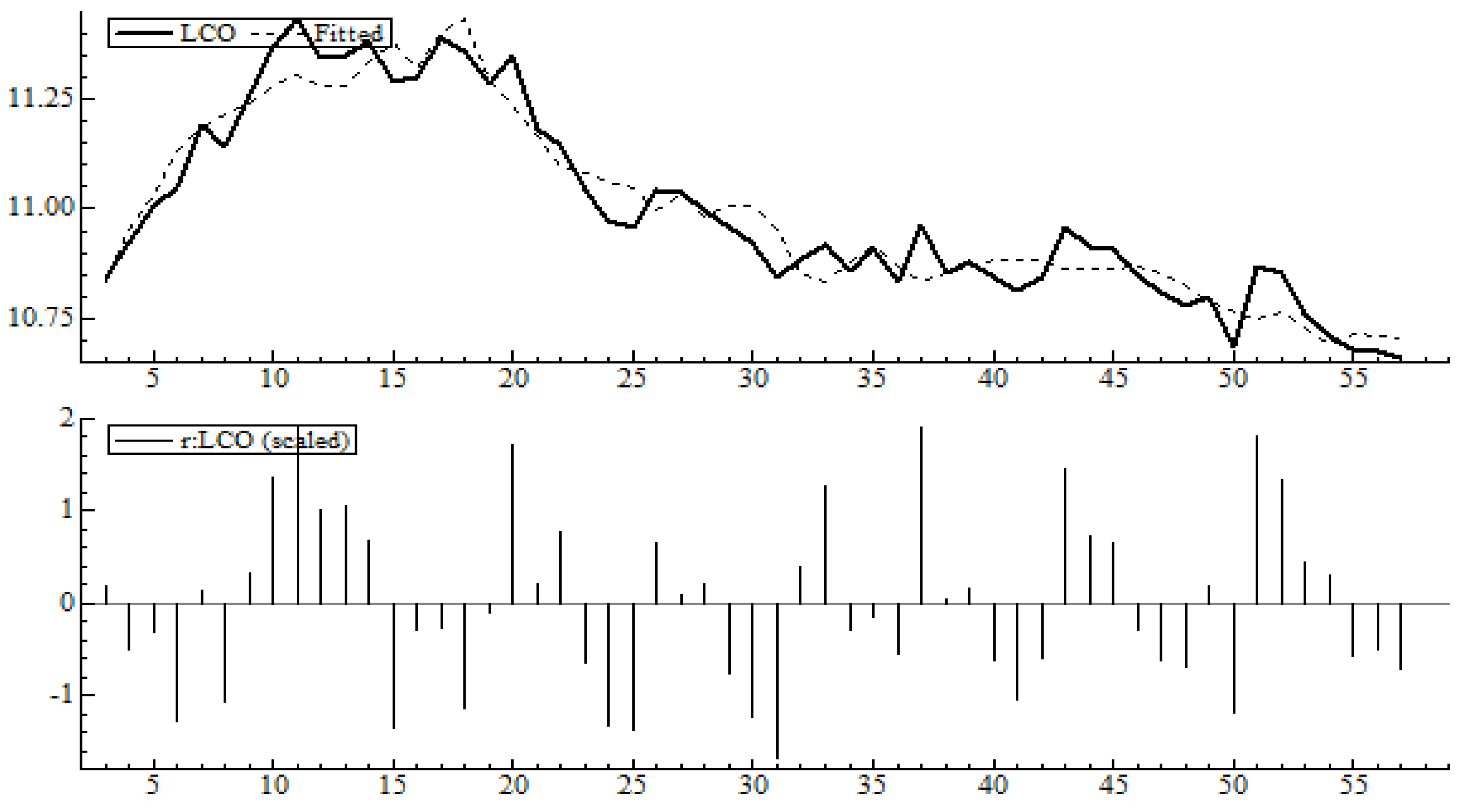
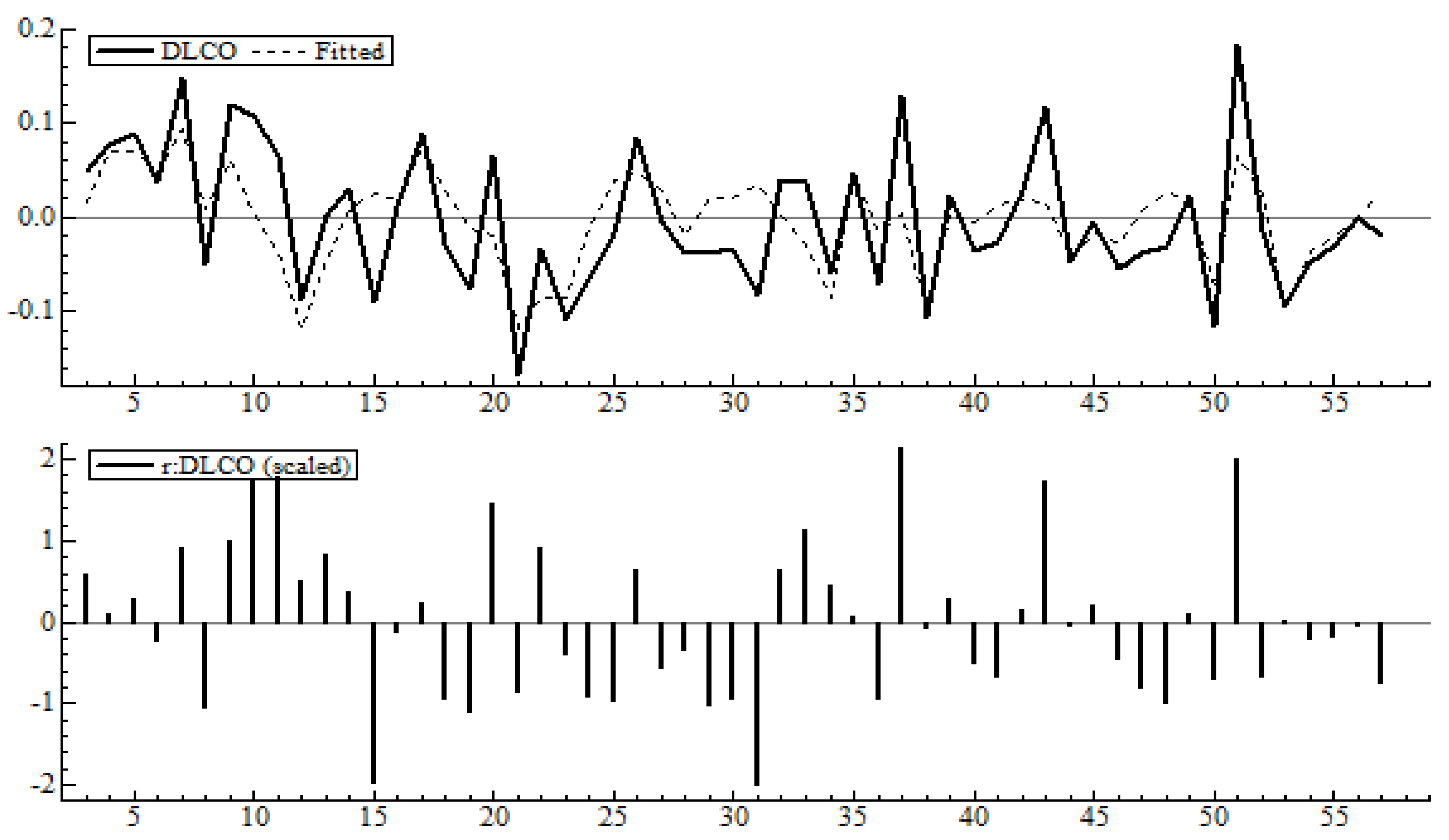
3.6. Model Performance

The Figure 3, Figure 4, Figure 5 and Figure 6 include model fitness for both the short- and long-term responses: the latter shows a better goodness of fit than the short-term models for both countries. The long-term model for Norway shows a better performance than that of Sweden: this more accurately explains the actual behavior of emissions (Figure 3 and Figure 5), while the performance of the short model of Norway also shows a superior performance to that of Sweden (Figure 4 and Figure 6).

The elasticities reported above (Table 5 and Table 6) can guide policy makers on how to design policy packages of both Sweden and Norway; the model results can help determine the right level of carbon and fuel taxes to cut emissions. However, our calculated elasticities are aggregated, while the taxes reported in Table 9 are disaggregated. The policy packages for cuts in GHG for both countries are discussed, with special emphasis on transport measures. Table 9, Table 10 and Table 11 tabulate the policy mix. The official policy mix (Table 9) does not include a quantitative analysis of the impacts of policy on CO₂ emissions.

To understand the role of green taxes (of which CO is the key one), it is essential to discuss the different tax instruments that are currently in use in both countries.

Table 9 shows the various green taxes for Sweden in 2019. The largest revenue comes from transport-related activity: rows for “Energy tax”, “carbon dioxide taxes” for transport, and “tax On transportation”. Transport-related taxes are high, i.e., ownership and road taxes. In sum, many green taxes mostly rely on transport-related taxes.

One key goal of the climate policy framework of Sweden is that first net zero emissions should be attained by 2045 and achieve negative growth after that year. The second emissions should be 85% lower than those of 1990 [51,52] (climate policy act; Climate Policy Council, 2020). To reduce emissions, the transport sector should be a key sector to decarbonize, since it is highly dependent on fossil fuels.

The Swedish Government has taken seven decisions, listed in Table 10, to mitigate climate change. A summary of these decisions for domestic transport, supported by the Climate Policy Act (Government Bill, 2019), are shown in Table 10. The government provides no quantitative assessment of several actions, i.e., carbon tax impacts, change in transport policy goals, funding for public charging infrastructure (renewable fuels and electricity sectors) and others. The “label “No” (in last Column) means that there is no government assessment of the measure listed in Table 10.

Norway’s green taxes that target climate change mitigation are tabulated in Table 11 based on [53]. The most important taxes are both the fuel tax and CO₂ taxes because of the volume of energy sold every year to power the transport sector. Some of these taxes are decades old, i.e., vehicle taxes date back to 1917 and road fuel taxes date to 1933. Vehicle taxes can complement CO₂ taxes to cut emissions.

Norway’s government is required to cut GHG emissions by 30% compared to 1990 (base year) by 2020. A cut of 40% by 2030 is also a target compared to the base year. By 2050, Norway needs to achieve cuts of 90–95% compared to the base year. These targets are hard to achieve without (a) decarbonizing transport and (b) using higher fuel or carbon taxes, which are already high by world standards. Our estimates on fuel tax, income and clean power (Table 5 and Table 6) can indicate how much these need to vary (Table 9, Table 10 and Table 11) to cut CO₂.

4. Discussion

4.1. Discussion on Sweden

Our econometric results (Section 3) confirm previous research. For the Swedish case, taxes are a powerful tool in cutting emissions [28], and indeed, our results (Table 5) confirm that fuel taxes are effective and high. Further evidence suggests that the carbon tax elasticity of demand for gasoline is three times larger than its price elasticity [6] for Sweden. Unlike Reference [6], we found that the fuel tax elasticity is stronger than the carbon tax elasticity. The authors of [6], however, used a different technique to ours and this may explain the differences in the results.

4.2. Discussion on Norway

In Norway’s case, the CO₂ tax effect was found to be modest in previous research [8]; however, we found that the CO₂ tax effect was larger than the fuel tax effect (Table 6, column one). For Norway, we found that the carbon price elasticity (“Dummy_CO₂tax”) shifted the emissions path much more than fuel tax elasticity (diesel tax).

Regarding the GDP effect on emissions, the channel is the income effect, which is easily influenced by a drop in economic activity or a financial crisis. One study [44] echoes the finding of Reference [43]: the financial crisis was the key factor for lower CO₂ emissions rather than the effects of CO₂ prices; that is, the assumption is made that the financial crisis reduced the demand for electricity and oil products. We failed to capture the effect of a drop in GDP: a fall in emissions after a rise in the income per capita variable for Sweden (Table 5 and Table 6). Instead, our results show that higher income is associated with higher emissions while, for Norway, a higher income is associated with technological change. The year dummy (Table 6) shows that the financial crisis of 2008–2009 significantly reduced emissions in Norway.

Macroeconomic studies for Norway and Sweden used the CGE framework [24], which assumes fixed prices and output and fixed substitution elasticities. Unlike these [24], our EqCM model does not assume fixed elasticities, or fixed prices. Instead, our models are based on time series datasets, which produce more realistic elasticity values. However, the high uncertainty in economic valuations of CO2 emissions and, thus, of taxes, remains [54,55], making it difficult to implement estimates from our EqCM analysis.

Our EqCM analysis captures the economic structure (the contribution of the manufacturing, services and primary sectors), explaining the differing path of emissions in both countries: Norway’s economy is highly reliant on its oil and gas sector, which fuels its emission growth. This is a fossil-fuel-dependent economy that behaves totally differently to Sweden: its emissions decline more rapidly over time, although, in per capita terms, Norway’s emissions are above the Swedish level. One lesson that can be drawn from the experience of these two nations is that high carbon and fuel taxes are insufficient to control the growth in fossil fuel use and a combination of measures is necessary to cut CO₂ emissions.

Since our model allows for a rough comparison between Sweden and Norway, we can say that the latter is an exception regarding the adoption of electric vehicles. Norway has become a global leader in the field of electromobility and the battery electric vehicle (BEV) market share is far higher than in any other country as a result of strong incentives promoting the purchase and ownership of BEVs. The role of incentives in promoting BEVs has been widely discussed in the literature, and makes Norway more of an outlier than a possible comparison.

Our econometric analysis faces three problems in the measurement of the effect of CO₂ taxes: the frequency of tax changes, tax exemptions and the “too many variables problem” [32]. However, since the analysis (Section 3) is estimated based on actual historical data, we can assume that some of these problems are partially solved. For example, the data on which our analysis is based ought to reflect the actual frequency of tax changes and exemptions; however, these exceptions would be indirectly captured in the fuel use levels.

Another notable comparison arising from our quantitative analysis of Sweden and Norway is that, in the future, both the fuel and CO₂ tax elasticities (Table 6 and Table 7) are likely to decrease in absolute value as drivers increasingly shift away from gasoline (diesel)-powered cars to electric ones. This will particularly apply to Norway since Norway is further ahead in the adoption of Battery electric vehicles (BEVs) than Sweden. In fact, the low level of fuel tax elasticity of Norway is partly explained by the success of BEVs. The success in the electrification of the vehicle stock of Norway is a result of subsidies for batteries and BEVs [56,57,58]. The growing adoption of BEVS in Norway explains the recent decline in emissions in Norway.

Future policy on the taxation of fossil fuels and of carbon will need to consider the fall in fossil fuel revenues, especially for transport fuels; such revenues will need to be recouped from other sources and from the new electric transport sector.

5. Conclusions

Our evidence shows that Norway, for most of the period of analysis, was less able to mitigate CO₂ emissions than Sweden due to non-tax factors. However, Norway’s adoption of BEVs implies that, in the future, the country will be well-placed to more easily cut emissions in the transport sector than Sweden.

Our quantitative and qualitative analysis confirms the three hypotheses based on an analysis of the cointegration of CO₂ emissions, fuel taxes, economic growth, and clean technologies of both countries. We found a cointegration relationship among variables for supply and demand, affecting CO₂ abatement efforts through the EqCM model and, since the series are cointegrated, we can confirm that there is an economic link among emissions and the other predictors. This new method allows for the determinants of emissions to be captured: a fast growth in emissions can be controlled with a target (a desired level of consumption) and an instrument (a tax).

Based on our model estimates, we found seven key outcomes for policy design.

▪

The first outcome of our considered policies is that the CO₂ tax has cut emissions in Norway more than in Sweden, but only in the first years following the introduction of the tax.

▪

Second the effect of the tax can be slow, since authorities use the tax as a revenue-raising device: in recessions, it will tend to rise, and in expansions it will decline. The tax will interact with (a) fuel taxes and (b) the rate of adoption of low-CO₂ technology. The tax’s effect on emissions, however, must be seen in relation to other policy measures that are introduced. For these reasons, the shifts in CO₂ taxes will not necessarily track emission cuts.

▪

Third, in both nations, the cuts in emissions occurred as a result of energy supply-side policies through nuclear power or hydropower generation.

▪

Fourth, the EqCM analysis shows that the effect of the tax on emissions is negative and permanent; however, the effect of technology (nuclear, renewables and hydro-power) is also essential to reduce emissions. Unlike Reference [6], we found that the diesel tax was more effective in cutting emissions than the direct CO₂ tax in both countries, but Norway’s diesel taxes were less powerful than those of Sweden, suggesting that higher taxes are needed in the former. The high personal income level explains the lower long-term price elasticity in Norway.

▪

Fifth, energy tax reform should also focus on other non-transport sectors; this reform will be needed since green tax revenue mostly relies on transport-related taxes, but the effectiveness of the latter may diminish after road electrification, which will lower tax revenue from transport energy (gasoline and diesel).

▪

Sixth, in Sweden, long-term emissions increase with economic growth. The response of emissions to fossil-fuel use is positive, as expected from a CO2-intensive energy source, but emissions respond negatively to (1) the CO₂ tax and fuel tax, (2) energy-efficiency measures, and (3) technology changes (i.e., nuclear power), as well as to (4) other unobservable effects. This is an R&D-led economy that is expected to produce lower growth rates of CO₂ emissions.

▪

Seventh, in Norway, emissions are still growing strongly despite enforced taxes on the supply side (oil and gas extraction) and the demand side. CO₂ emissions move in opposing directions: taxes, effective carbon prices and income effects and technological changes lead to cuts in emissions, while oil extraction activities and transport activities push up emissions. The long-term responses of emissions to economic growth, CO₂ prices and fuel taxes ensure that emissions decline.

▪

Future work is needed to examine further ways to cut emissions in the transport sector. Our analysis reveals that policy ought to focus on the greater electrification of transport for both nations, a reduction in energy use for road transport (Norway) and a removal of tax exemptions for industry, including carbon taxes.

References

1. Hendry, D.F. Equilibrium correction models. In The New Palgrave Dictionary in Economics; Palgrave Macmillan: London, UK, 2008; pp. 1–11. [Google Scholar]
2. Nelson, C.; Ploser, C. Trends and Random Walks in Macroeconomic Time Series: Some Evidence and Implications. J. Monet. Econ. 1982, 10, 139–169. [Google Scholar] [CrossRef]
3. Turnovsky, S. Stabilization theory and policy: 50 years after the Phillips curve. Economica 2011, 78, 67–88. [Google Scholar] [CrossRef]
4. Phillips, A.W.H. Stabilization policy in a closed economy. Econ. J. 1954, 64, 290–333. [Google Scholar] [CrossRef]
5. Phillips, A.W.H. Stabilization policy and the time form of lagged response. Econ. J. 1957, 67, 265–277. [Google Scholar] [CrossRef]
6. Andersson, J. Carbon Taxes and CO2 Emissions: Sweden as a Case Study. Am. Econ. J. Econ. Policy 2019, 11, 1–30. [Google Scholar] [CrossRef] [Green Version]
7. Metcalf, G.E.; Stock, J.H. Measuring the Macroeconomic Impacts of Carbon Taxes. Am. Econ. Rev. Pap. Proc. 2020, 110, 101–106. [Google Scholar] [CrossRef]
8. Bruvoll, A.; Larsen, M. Greenhouse gas emissions in Norway: Do carbon taxes work? Energy Policy 2004, 32, 493–505. [Google Scholar] [CrossRef] [Green Version]
9. Agnolucci, P.; Barker, T.; Ekins, P. Hysteresis and Energy Demand: The Announcement Effects of the UK Climate Change Levy; UKERC: London, UK, 2004; pp. 1–16. [Google Scholar]
10. Bohlin, F. The Swedish Carbon Dioxide tax: Effects on Biodiesel Use and Carbon Dioxide Emissions. Biomass Bioenergy 1998, 15, 283–291. [Google Scholar] [CrossRef]
11. Ekins, P.; Barker, T. Carbon Taxes and Carbon Emission Trading. J. Econ. Surv. 2001, 15, 325–376. [Google Scholar] [CrossRef]
12. Harju, J.; Kosonen, T.; Laukkanen, M.; Palanne, K. The Heterogenous Incidence of Fuel Carbon Taxes: Evidence From Fuel Station Level Data. J. Environ. Econ. Manag. 2022, 112, 2–33. [Google Scholar] [CrossRef]
13. Rivers, N.; Schaufele, B. Salience of Carbon Taxes in the Gasoline Market. J. Environ. Econ. Manag. 2015, 74, 23–36. [Google Scholar] [CrossRef]
14. Metcalf, G.E. On the Economics of a Carbon Tax for the United States. Brook. Pap. Econ. Act. 2019, 1, 405–458. [Google Scholar] [CrossRef]
15. Prettis, F. Does a Carbon Tax Reduce CO2 Emissions? Evidence from British Columbia; Department of Economics, University of Victoria: Victoria, BC, Canada, 2019. [Google Scholar]
16. Pigou, A.C. A Study in Public Finance; Macmillan & Co., Ltd.: New York, NY, USA, 1929; Volume 17, pp. 1–323. [Google Scholar]
17. Weitzman, M.L. Prices vs. Quantities. Rev. Econ. Stud. 1974, 41, 477–491. [Google Scholar] [CrossRef]
18. Baumol, W.; Oates, W. The Theory of Environmental Policy (pp. I–IV); Cambridge University Press: Cambridge, UK, 1988; pp. 1–312. [Google Scholar]
19. Nordhaus, W. A Question of Balance: Weighing the Options on Global Warming Policies; Yale University Press: New Haven, CT, USA, 2008; pp. 1–234. [Google Scholar]
20. Manne, A.; Richels, R. Buying Greenhouse Insurance: The Economic costs of CO2 emissions limits; MIT Press: Cambridge, MA, USA, 1992; pp. 1–194. [Google Scholar]
21. Criqui, P.; Kouvartakis, N.; Scharttonenholzer, L. The impacts of carbon constraint on power generation and renewable energy technologies. In Sectoral Economic Costs and Benefits of GHG Mitigation: Proceedings of an IPCC Expert Meeting, Eisenach, Germany, 14–15 February 2000; Bernstein, L., Pan, J., Eds.; Technical support Unit, IPCC working Group III: Geneva, Switzerland, 2000. [Google Scholar]
22. Barker, T.; Scrieciu, S. Modeling Low Climate Stabilization with E3MG: Towards a ‘New Economics’ Approach to Simulating Energy-Environment-Economy System Dynamics. Energy J. Int. Assoc. Energy Econ. 2010, 31, 137–164. [Google Scholar] [CrossRef]
23. Hendry, D.F.; Pretis, F. Anthropogenic influences on atmospheric CO2. In Energy and Climate Change; Fouqet, R., Ed.; Edward Elgar: Cheltenham, UK, 2013; pp. 287–327. [Google Scholar]
24. Kverndokk, S.; Rosendahl, K.E. CO2 Mitigation Costs and Ancillary Benefits in the Nordic Countries, the UK and Ireland: A Survey. Memorandum. Department of Economics, University of Oslo: Oslo, Norway, 2000; pp. 1–53. [Google Scholar]
25. Pesaran, H.; Smith, R. Structural analysis and cointegrating vars. J. Econ. Surv. 1998, 12, 471–505. [Google Scholar] [CrossRef]
26. Carattini, S.; Baranzini, A.; Thalmann, P.; Varone, P.; Vöhringer, F. Green Taxes in a post-Paris World: Are Millions of Nays Inevitable? Environ. Resour. Econ. 2017, 68, 97–128. [Google Scholar] [CrossRef] [Green Version]
27. Wondgagegn, T.; Gren, I.M. Road fuel demand and regional effects of carbon taxes in Sweden. Energy Policy 2020, 144, 111648. [Google Scholar]
28. Sterner, T. Political Economy Obstacles to Fuel Taxation. Energy J. 2004, 25, 1–18. [Google Scholar]
29. Brannlund, R.; Lundgren, T. Environmental Policy and Profitability—Evidence from Swedish Industry. Environ. Econ. Policy Stud. 2010, 12, 59–78. [Google Scholar] [CrossRef]
30. Lundgren, T.; Marklund, P.-O.; Climate Policy and Profit Efficiency. CERE Working Paper No. 11. Umea: Centre for Environmental and Resource Economics. Available online: http://www.cere.se/ironmental (accessed on 15 May 2018).
31. Brannlund, R.; Lundgren, T.; Marklund, P.-O. Carbon Intensity in Production and the Effects of Climate Policy—Evidence from Sweden. Energy Policy 2014, 67, 844–857. [Google Scholar] [CrossRef]
32. Andersen, M.S. Vikings and virtues-a decade of CO2 taxation. Clim. Policy 2004, 4, 13–24. [Google Scholar] [CrossRef] [Green Version]
33. Productivity Commission. Carbon Emission Policies in Key Economies, Research Report. 2011. Canberra, Australia. October. pp. 1–760. Available online: http://www.pc.gov.au/inquiries/completed/carbon-prices/report (accessed on 10 January 2014).
34. Bjorner, T.; Jensen, H.H. Energy taxes, voluntary agreements and investment subsidies—A micro-panel analysis of the effect on Danish industrial companies’ energy demand. Resour. Energy Econ. 2004, 24, 229–249. [Google Scholar] [CrossRef]
35. OECD. Taxing Energy Use: A Graphical Analysis; Report: Paris, France, 2018. [Google Scholar]
36. Laing, T.; Misato, S.; Grubb, M.; Comberti, C. Assessing the Effectiveness of the Emissions Trading Scheme (ETS); Working Paper 106; Grantham Research Institute of Climate Change and the Environment: London, UK, 2013; pp. 1–35. [Google Scholar]
37. Ellerman, A.D.; Buchner, B. Over-Allocation or Abatement? A Preliminary Analysis of the EU ETS Based on the 2005–06 Emissions Data. Environ. Resour. Econ. 2008, 41, 267–287. [Google Scholar] [CrossRef] [Green Version]
38. Anderson, B.; Di Maria, C. Abatement and Allocation in the Pilot Phase of the EU ETS. Environ. Resour. Econ. 2011, 48, 83–101. [Google Scholar] [CrossRef] [Green Version]
39. Fezzy, C.; Bunn, D. Structural interactions of European carbon prices. J. Energy Mark. 2009, 24, 53–69. [Google Scholar] [CrossRef]
40. Jaraite, J.; Kazukauskas, A.; Lundgren, T. The effects of climate policy on environmental expenditure and investment: Evidence from Sweden. J. Environ. Econ. Policy 2014, 3, 148–166. [Google Scholar] [CrossRef]
41. Broberg, T.; Marklund, P.-O.; Samakovlis, E. Testing the Porter Hypothesis: The Effects of Environmental Investments on Efficiency in Swedish Industry. J. Product. Anal. 2013, 40, 43–56. [Google Scholar] [CrossRef]
42. World Bank. State and Trends of Carbon Pricing; Report, p. 94; World Bank, Ecofys and Vivid Economics: Washington, DC, USA, 2019. [Google Scholar]
43. Declerq, B.; Delarue, E.; D’haeseleer, W. Impact of the economic recession on the European power sectors CO2 emissions. Energy Policy 2011, 39, 1677–1686. [Google Scholar] [CrossRef]
44. Cambridge Econometrics. An Impact Assessment of the Current Economic Downturn on UK CO2 Emissions: A final report for the Committee on Climate Change; The Committee on Climate Change: London, UK, 2009. [Google Scholar]
45. Statistics Sweden. Environmental Taxes. 2020. Available online: http://www.scb.se/en_/Findingstatistics/Statistics-by-subject-area/Environment/Environmental-accounts-andsustainable-development/System-of-Environmental-and-Economic-Accounts/Aktuell-Pong/38171/Environmental-taxes/271568/ (accessed on 3 March 2017).
46. World Bank. World Development Indicators. Available online: https://databank.worldbank.org/source/world-development-indicators (accessed on 10 February 2020).
47. UN. Statistics. 2019. Available online: http://data.un.org/ (accessed on 2 October 2019).
48. Statistics Norway. National Accounts 1978–1996 (Various Years), Official Statistics of Norway. 2020. Available online: https://www.ssb.no/en/forside;jsessionid=4CD26C5C8D4E3B34AF695B73C56CB126.kpld-as-prod03?hide-from-left-menu=true&language-code=en&menu-root-alternative-language=true (accessed on 3 March 2017).
49. IEA (International Energy Agency). Carbon Emissions from Fuel Combustion; Edition. Various years; OECD: Paris, France, 2013; p. 417. [Google Scholar]
50. Swedish Energy Agency. Economic Instruments in Environmental Policy. Stockholm. Sweden: Swedish Environmental Protection Agency and the Swedish Energy Agency. Available online: https://www.energimyndigheten.se/en/ (accessed on 20 May 2018).
51. Government Bill. 20.65. En Samlad politik for klimatet-klimatpolitisk handlingsplan 2019. Available online: https://eef.se/wp-content/uploads/2019/12/Klimatpolitisk-handlingsplan-prop.-dec-2019.pdf (accessed on 12 December 2019).
52. Swedish Climate Policy Council. Klimatpolitiska Radet. 2020. Available online: https://www.klimatpolitiskaradet.se/en (accessed on 12 December 2019).
53. Norwegian Ministry of Climate and Environment. Norway’s Fourth Biennal Report. Under the framework Convention on Climate Change; Status Report: Oslo, Norway, 2020; p. 92.
54. Nocera, S.; Cavallaro, F. Economic Evaluation of Future Carbon Impacts on the Italian Highways. Procedia Soc. Behav. Sci. 2012, 54, 1360–1369. [Google Scholar] [CrossRef] [Green Version]
55. Nocera, S.; Tonin, S. A Joint Probability Density Function for reducing the Uncertainty of Marginal Social Cost of Carbon Evaluation in Transport Planning. Adv. Intell. Syst. Comput. 2014, 262, 113–126. [Google Scholar]
56. Holtsmark, B.; Skonhoft, A. The Norwegian support and subsidy policy of electric cars. Should it be adopted by other countries? Environ. Sci. Policy 2014, 42, 160–168. [Google Scholar] [CrossRef]
57. Olson, E.L. The financial and environmental costs and benefits for Norwegian electric car subsidies: Are they good public policy? Int. J. Technol. Policy Manag. 2015, 15, 277–296. [Google Scholar] [CrossRef] [Green Version]
58. Bjerkan, K.Y.; Nørbech, T.E.; Nordtømme, M.E. Incentives for promoting Battery Electric Vehicle (BEV) adoption in Norway. Transp. Res. Part D Transp. Environ. 2016, 43, 169–180. [Google Scholar] [CrossRef] [Green Version]
59. Hill, R.C.; Griffith, W.E.; Lim, G.C. Principles of Econometrics, 5th ed.; Wiley: Hoboken, NJ, USA, 2018; pp. 1–192. [Google Scholar]
Figure 3. Results for the Sweden long-term model: 1. See Equation (1). Fitted model top graph, residuals bottom graph.
Energies 15 03885 g003
Figure 4. Results for the Sweden short-term model: 2. See Equation (2).
Energies 15 03885 g004
Figure 5. Results for the long-term model of CO2 emissions (Norway): 3. See Equation (4). Fitted model top graph; residuals bottom graph.
Energies 15 03885 g005
Figure 6. Results for the short-term model of CO2 emissions (Norway): See Equation (5). Fitted model top graph; residuals bottom graph.
Energies 15 03885 g006