
Overview of Battery Impedance Modeling Including Detailed State-of-the-Art Cylindrical 18650 Lithium-Ion Battery Cell Comparisons †

 , , , and
Abstract
:1. Introduction
2. Recent Research on 18650 Lithium-Ion Battery Cells
3. Battery Modeling and Parameter Extraction Using Electrochemical Impedance Spectroscopy
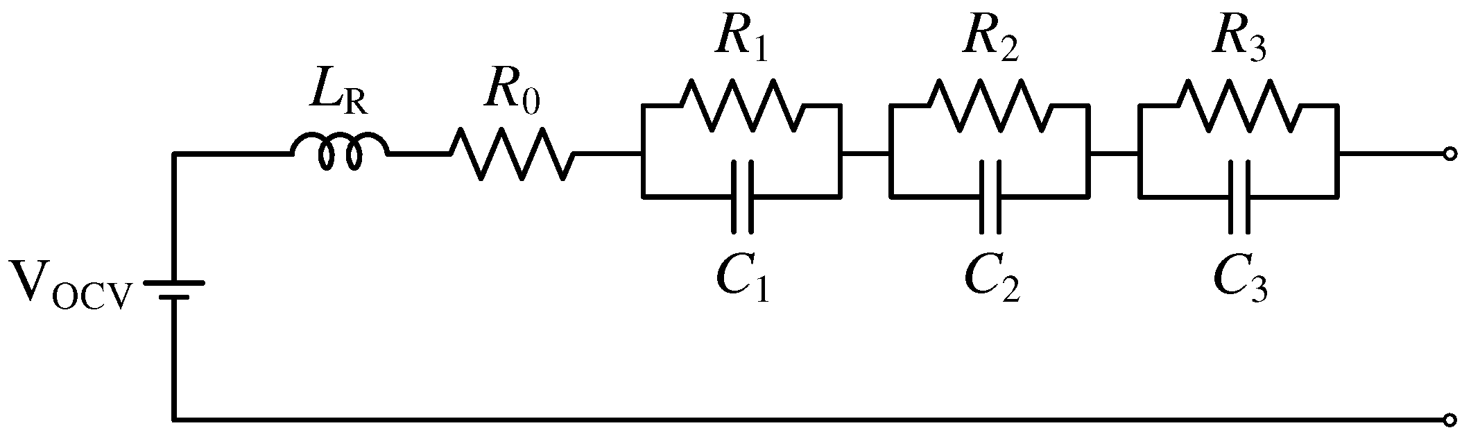
3.1. Battery Modeling
3.1.1. RC-Link Models
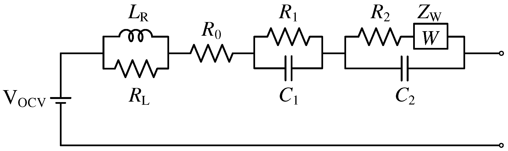
3.1.2. Warburg Model
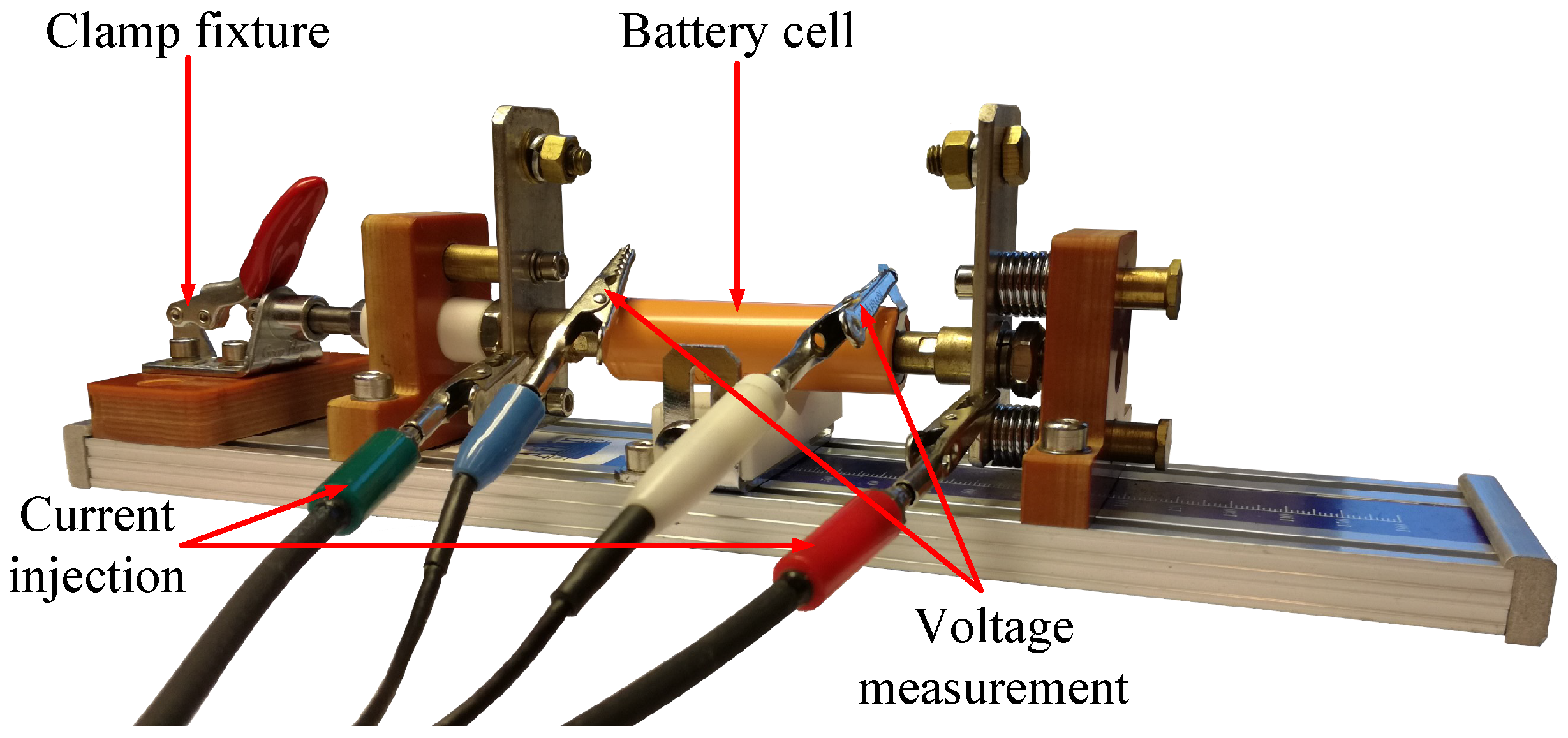
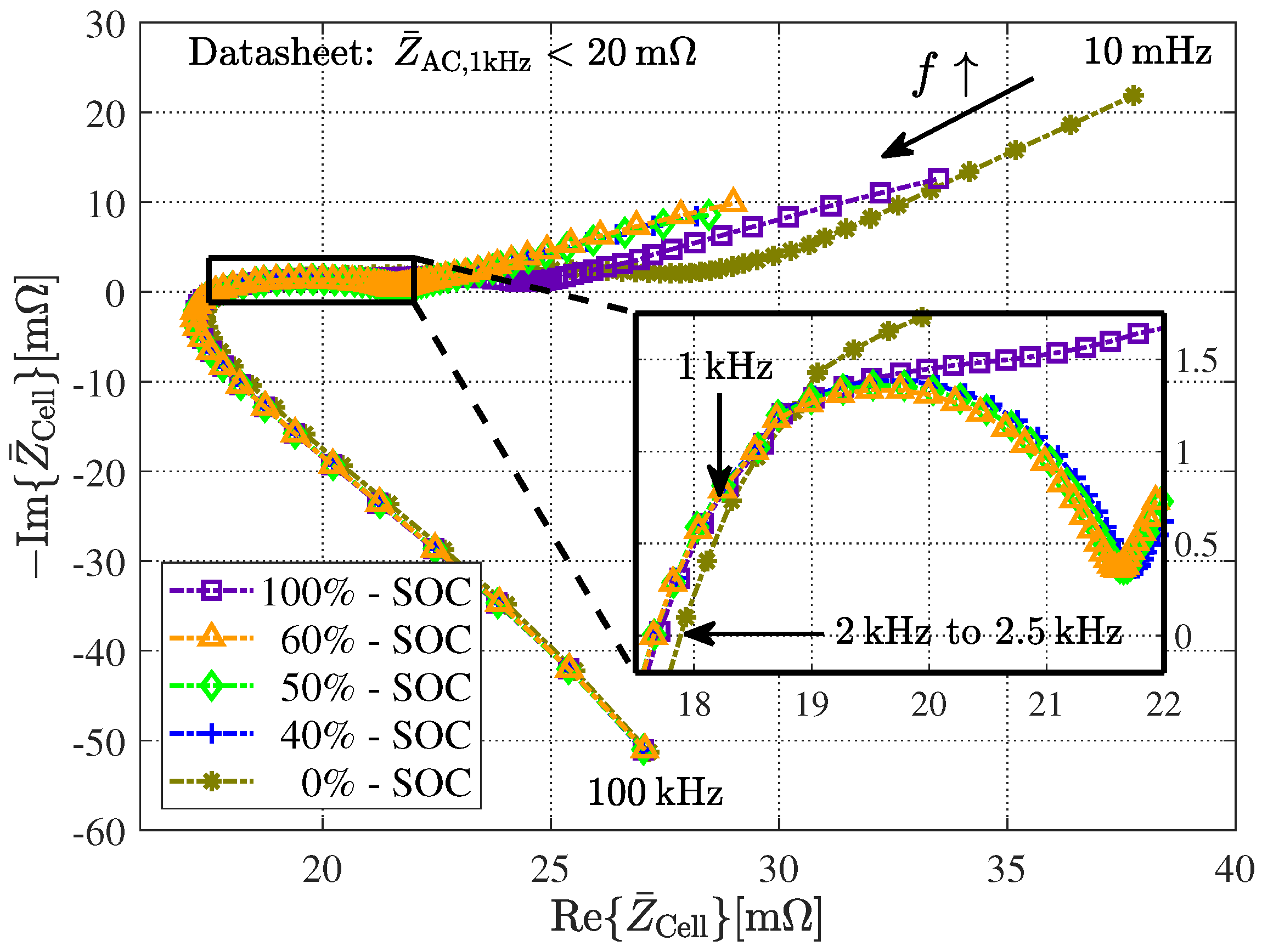
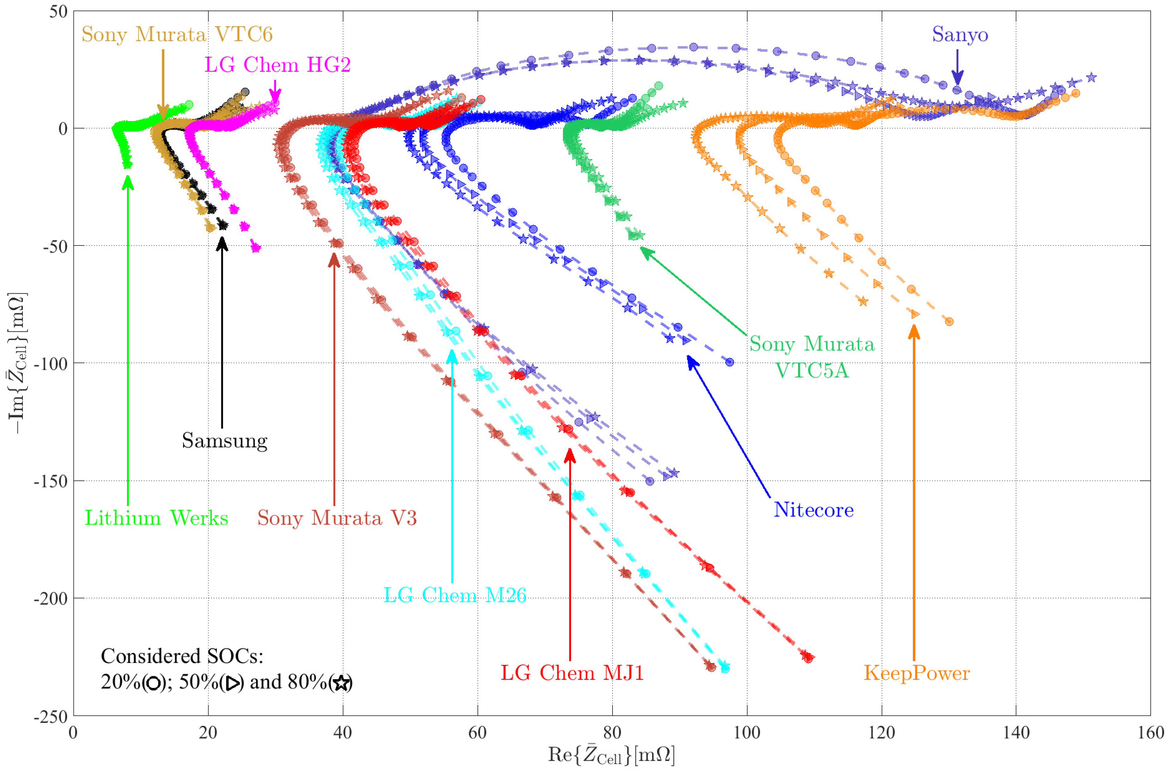
3.2. Electrochemical Impedance Spectroscopy
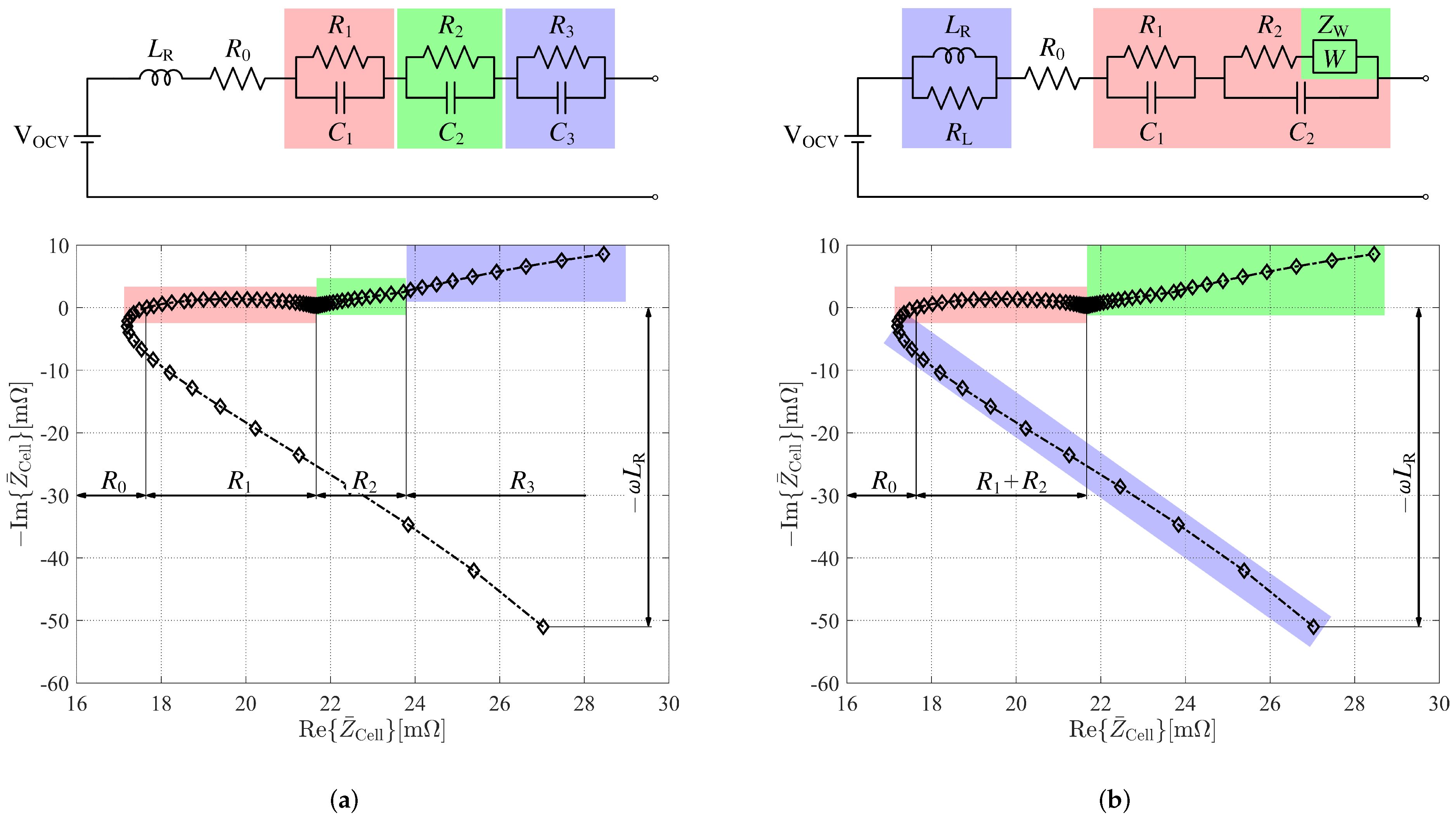
3.3. Parameter Extraction
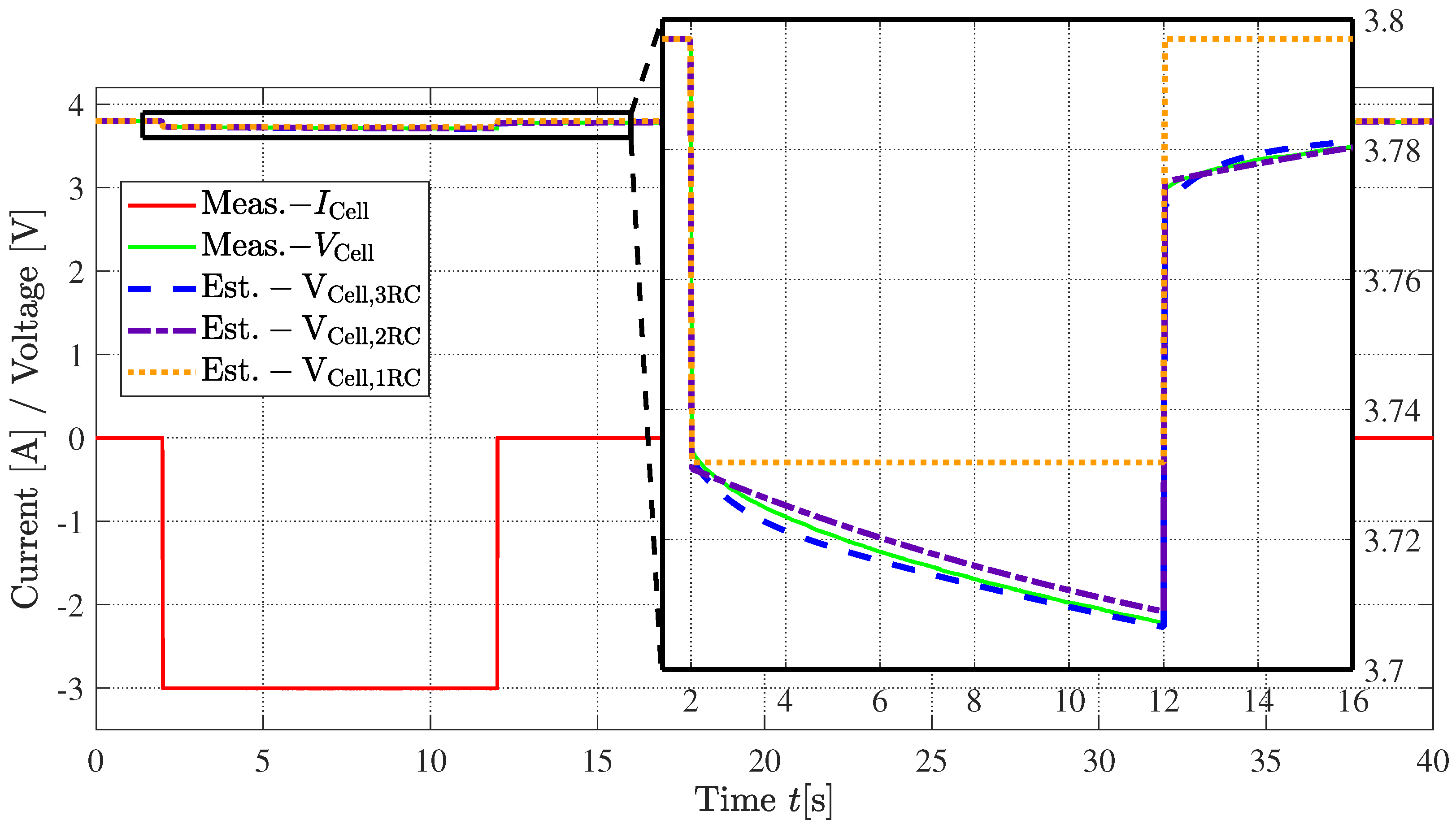
3.4. Simulation in Time-Domain
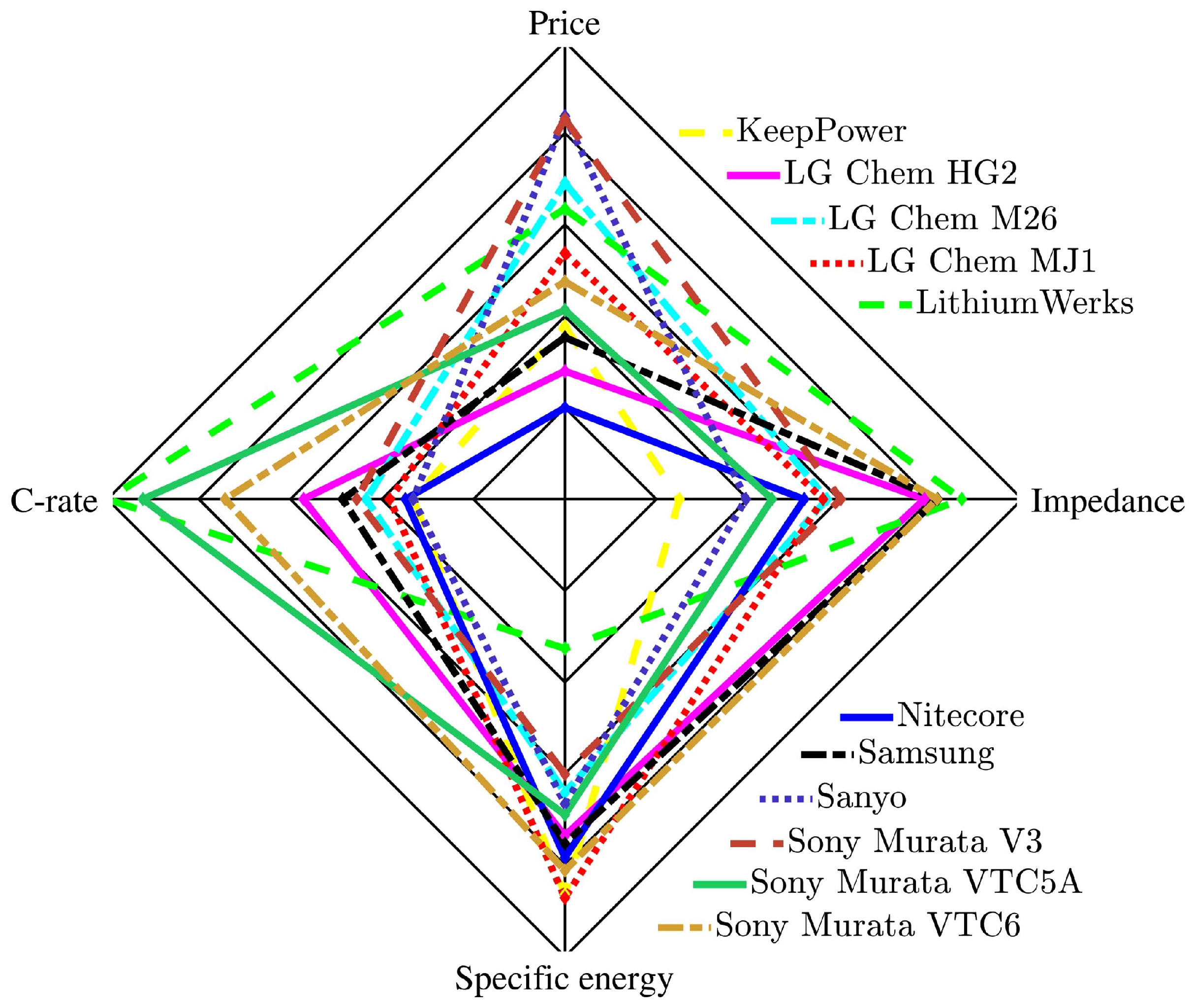
4. Battery Cell Comparisons

| Manufacturer | Model | Capacity Q [mAh] | Voltage [V] | C-Rate | Spec. Energy | Price [USD] |
|---|---|---|---|---|---|---|
| Keeppower | P1834J | 3400 | 3.7 | 2 | 262.08 | 11.53 |
| LG Chem | HG2 | 3000 | 3.6 | 6.7 | 226.53 | 14.43 |
| LG Chem | M26 | 2600 | 3.65 | 4 | 200.42 | 5.45 |
| LG Chem | MJ1 | 3500 | 3.635 | 3 | 264.29 | 8.43 |
| Lithium Werks | M1B | 2500 | 3.3 | 28 | 112.89 | 6.55 |
| Murata | V3 | 2250 | 3.7 | 4.4 | 189.20 | 2.73 |
| Murata | VTC5A | 2250 | 3.7 | 13.5 | 213.78 | 10.85 |
| Murata | VTC6 | 3120 | 3.7 | 10 | 247.73 | 9.64 |
| Nitecore | NL1835HP | 3500 | 3.6 | 2.3 | 239.81 | 29.04 |
| Samsung | 30Q | 3000 | 3.6 | 5 | 231.25 | 12.01 |
| Sanyo | ZT | 2700 | 3.7 | 2 | 207.26 | 2.61 |
| Manufacturer | Model | ||||||||
|---|---|---|---|---|---|---|---|---|---|
| Keeppower | P1834J | 147.40 | 250.73 | 100.07 | 6.90 | 1.06 | 8.16 | 0.08 | 1.96 |
| LG Chem | HG2 | 88.88 | 251.07 | 17.76 | 1.00 | 1.84 | 2.49 | 0.18 | 1.80 |
| LG Chem | M26 | 409.17 | 882.39 | 40.66 | 5.91 | 0.24 | 1.64 | 3.77 | 2.00 |
| LG Chem | MJ1 | 410.74 | 755.26 | 43.93 | 4.47 | 0.35 | 0.09 | 28.79 | 1.91 |
| Lithium Werks | V3 | 25.78 | 145.36 | 6.63 | 0.72 | 11.22 | 1.59 | 0.27 | 1.86 |
| Murata | V3 | 414.44 | 816.17 | 33.86 | 1.81 | 5.64 | 7.05 | 0.19 | 2.46 |
| Murata | VTC5A | 79.91 | 208.19 | 73.56 | 3.05 | 0.16 | 1.61 | 1.26 | 1.70 |
| Murata | VTC6 | 74.23 | 209.11 | 12.74 | 1.38 | 1.51 | 3.30 | 0.13 | 1.76 |
| Nitecore | NL1835HP | 187.59 | 226.58 | 53.67 | 5.38 | 1.59 | 8.23 | 0.13 | 2.17 |
| Samsung | 30Q | 73.97 | 178.70 | 13.24 | 2.57 | 0.16 | 0.78 | 1.81 | 1.98 |
| Sanyo | ZT | 274.49 | 476.19 | 41.10 | 30.18 | 0.10 | 48.17 | 0.44 | 4.47 |
| Manufacturer | Model | ||||||||
|---|---|---|---|---|---|---|---|---|---|
| Keeppower | P1834J | 136.71 | 99.10 | 9.53 | 67.71 | 7.85 | 1.29 | 16.93 | 1033.82 |
| LG Chem | HG2 | 86.38 | 17.41 | 4.11 | 157.65 | 2.60 | 347.27 | 19.80 | 1391.13 |
| LG Chem | M26 | 389.73 | 38.15 | 9.68 | 128.17 | 2.43 | 77.34 | 23.67 | 1057.06 |
| LG Chem | MJ1 | 357.66 | 40.95 | 7.23 | 808.75 | 0.60 | 2.11 | 9.85 | 2428.49 |
| Lithium Werks | M1B | 24.58 | 6.41 | 1.91 | 902.01 | 1.49 | 19.27 | 4.73 | 4432.25 |
| Murata | V3 | 399.52 | 29.91 | 4.82 | 42.58 | 8.97 | 0.20 | 11.13 | 406.26 |
| Murata | VTC5A | 72.75 | 73.36 | 5.14 | 150.13 | 1.96 | 390.15 | 19.26 | 1291.63 |
| Murata | VTC6 | 67.50 | 12.51 | 5.26 | 129.85 | 2.28 | 4047.82 | 20.65 | 1344.85 |
| Nitecore | NL1835HP | 143.74 | 52.41 | 9.36 | 97.67 | 6.79 | 1.60 | 17.61 | 850.42 |
| Samsung | 30Q | 72.70 | 12.98 | 1.83 | 123.45 | 2.24 | 0.14 | 15.08 | 861.11 |
| Sanyo | ZT | 261.80 | 39.80 | 40.58 | 828.57 | 18.32 | 499.70 | 43.43 | 0.10 |
| Manufacturer | Model | ||||||
|---|---|---|---|---|---|---|---|
| Keeppower | P1834J | 136.55 | 99.90 | 15.55 | 128.77 | 15.13 | 884.67 |
| LG Chem | HG2 | 86.37 | 17.48 | 4.53 | 175.10 | 14.74 | 985.19 |
| LG Chem | M26 | 389.91 | 38.32 | 10.47 | 142.26 | 19.31 | 895.38 |
| LG Chem | MJ1 | 357.66 | 40.95 | 7.83 | 434.08 | 4.94 | 1361.57 |
| Lithium Werks | M1B | 25.75 | 6.36 | 2.85 | 363.34 | 11.85 | 859.94 |
| Murata | V3 | 399.65 | 30.65 | 12.75 | 123.38 | 16.67 | 681.21 |
| Murata | VTC5A | 78.66 | 73.11 | 5.35 | 151.62 | 15.12 | 1015.36 |
| Murata | VTC6 | 73.61 | 12.14 | 5.41 | 130.77 | 15.04 | 995.59 |
| Nitecore | NL1835HP | 169.14 | 52.30 | 15.86 | 154.31 | 17.04 | 813.53 |
| Samsung | 30Q | 72.80 | 12.62 | 4.43 | 137.29 | 15.36 | 872.87 |
| Sanyo | ZT | 235.60 | 38.02 | 87.16 | 509.41 | 22.89 | 1138.59 |
| Manufacturer | Model | ||||
|---|---|---|---|---|---|
| Keeppower | P1834J | 136.63 | 99.49 | 3.43 | 131.24 |
| LG Chem | HG2 | 86.37 | 17.44 | 4.29 | 165.40 |
| LG Chem | M26 | 389.91 | 38.28 | 10.11 | 138.14 |
| LG Chem | MJ1 | 384.75 | 41.46 | 7.27 | 151.23 |
| Lithium Werks | M1B | 25.56 | 6.66 | 2.77 | 498.62 |
| Murata | V3 | 391.38 | 31.52 | 11.49 | 121.36 |
| Murata | VTC5A | 77.25 | 73.37 | 5.24 | 159.57 |
| Murata | VTC6 | 72.11 | 12.53 | 5.33 | 135.56 |
| Nitecore | NL1835HP | 163.25 | 52.67 | 14.68 | 147.01 |
| Samsung | 30Q | 71.17 | 12.97 | 4.11 | 147.28 |
| Sanyo | ZT | 255.02 | 41.93 | 76.10 | 144.48 |
5. Conclusions
Author Contributions
Funding
Conflicts of Interest
Abbreviations
| EIS | Electrochemical impedance spectroscopy |
| ECM | Equivalent circuit model |
| Est | Estimated |
| NMC | Nickel–manganese–cobalt–oxide |
| RMS | Root mean square |
| SOC | State of charge |
Appendix A
| f | Re{} | −Im{} | f | Re{} | −Im{} | f | Re{} | −Im{} |
|---|---|---|---|---|---|---|---|---|
| 100,078.1 | 0.1248685 | 0.0791728 | 397.9953 | 0.1025465 | −0.0037484 | 1.584686 | 0.1158481 | −0.0014265 |
| 79,453.13 | 0.1192303 | 0.0660843 | 315.5048 | 0.103217 | −0.0039928 | 1.266892 | 0.1159938 | −0.0013244 |
| 63,140.62 | 0.1147977 | 0.0549908 | 252.4038 | 0.1038846 | −0.0041895 | 0.999041 | 0.1161152 | −0.001245 |
| 50,203.12 | 0.1113422 | 0.0456027 | 198.6229 | 0.1046293 | −0.0043773 | 0.7923428 | 0.1162334 | −0.0011867 |
| 39,890.62 | 0.108636 | 0.0378051 | 158.3615 | 0.1053615 | −0.0045084 | 0.633446 | 0.1163523 | −0.0011659 |
| 31,640.63 | 0.1064436 | 0.0313035 | 125.558 | 0.1061272 | −0.0046076 | 0.5040323 | 0.1164643 | −0.0011691 |
| 25,171.88 | 0.1046336 | 0.0260184 | 100.4464 | 0.1068876 | −0.0046767 | 0.400641 | 0.116578 | −0.0012005 |
| 20,015.62 | 0.1030744 | 0.0215612 | 79.00281 | 0.1077005 | −0.0046817 | 0.316723 | 0.1166854 | −0.0012651 |
| 15,890.62 | 0.101749 | 0.0177461 | 63.3446 | 0.1084316 | −0.0046515 | 0.2520161 | 0.1168034 | −0.0013556 |
| 12,609.37 | 0.1006624 | 0.0144373 | 50.22321 | 0.1092287 | −0.0045741 | 0.2003205 | 0.1169279 | −0.001486 |
| 10,078.13 | 0.0998588 | 0.0116388 | 38.42213 | 0.1100764 | −0.0044632 | 0.1588983 | 0.1170757 | −0.0016525 |
| 8015.625 | 0.0992723 | 0.0091599 | 31.25 | 0.1107429 | −0.0043228 | 0.1260081 | 0.1172597 | −0.0018626 |
| 6328.125 | 0.0989084 | 0.0069591 | 24.93351 | 0.1114179 | −0.0041403 | 0.1001603 | 0.117478 | −0.0021162 |
| 5015.625 | 0.0987513 | 0.0051215 | 19.86229 | 0.1121067 | −0.0039256 | 0.0794492 | 0.1177547 | −0.0024267 |
| 3984.375 | 0.0987152 | 0.0035754 | 15.625 | 0.1127404 | −0.0036522 | 0.0631739 | 0.1178996 | −0.0028201 |
| 3170.956 | 0.0988392 | 0.0022968 | 12.40079 | 0.1132926 | −0.0033823 | 0.0501337 | 0.1181734 | −0.0032702 |
| 2527.573 | 0.0990051 | 0.0012205 | 9.93114 | 0.1137499 | −0.0031128 | 0.0398258 | 0.1185147 | −0.0038034 |
| 1976.103 | 0.0993063 | 0.0002402 | 7.944915 | 0.1141792 | −0.002829 | 0.0316296 | 0.1189262 | −0.0044321 |
| 1577.524 | 0.0996115 | −0.0005684 | 6.317385 | 0.1145427 | −0.0025496 | 0.0251206 | 0.1194369 | −0.0051677 |
| 1265.625 | 0.1000291 | −0.0012188 | 5.008013 | 0.1148783 | −0.0022777 | 0.0199553 | 0.1200348 | −0.0060106 |
| 998.264 | 0.1004754 | −0.0018054 | 3.945707 | 0.1151497 | −0.0020308 | 0.0158522 | 0.1207429 | −0.0069609 |
| 796.875 | 0.1009431 | −0.0022927 | 3.158693 | 0.1153695 | −0.001831 | 0.0125907 | 0.1216125 | −0.0080523 |
| 627.7902 | 0.1014475 | −0.0027202 | 2.504006 | 0.1155009 | −0.0017247 | 0.0100011 | 0.122649 | −0.0092733 |
| 505.5147 | 0.1018677 | −0.0034748 | 1.998082 | 0.1156775 | −0.0015757 |
| f | Re{} | −Im{} | f | Re{} | −Im{} | f | Re{} | −Im{} |
|---|---|---|---|---|---|---|---|---|
| 100,078.1 | 0.1092766 | 0.2248998 | 397.9953 | 0.0434193 | −0.0014255 | 1.584686 | 0.0488809 | −0.0006845 |
| 79,453.13 | 0.0943386 | 0.1867189 | 315.5048 | 0.0439041 | −0.0017356 | 1.266892 | 0.0489755 | −0.0007088 |
| 63,140.62 | 0.0823958 | 0.1547544 | 252.4038 | 0.0443739 | −0.0019448 | 0.999041 | 0.0490154 | −0.0007727 |
| 50,203.12 | 0.073147 | 0.1278604 | 198.6229 | 0.0448717 | −0.0020896 | 0.7923428 | 0.0490972 | −0.0008471 |
| 39,890.62 | 0.0659943 | 0.1053338 | 158.3615 | 0.0453303 | −0.0021585 | 0.633446 | 0.0492239 | −0.0009284 |
| 31,640.63 | 0.0604904 | 0.0865721 | 125.558 | 0.0457481 | −0.0021713 | 0.5040323 | 0.0493204 | −0.0010369 |
| 25,171.88 | 0.0562198 | 0.0713342 | 100.4464 | 0.0461982 | −0.0021252 | 0.400641 | 0.0494389 | −0.0011674 |
| 20,015.62 | 0.0527559 | 0.0587981 | 79.00281 | 0.0466082 | −0.0020387 | 0.316723 | 0.049575 | −0.0013207 |
| 15,890.62 | 0.049846 | 0.0483892 | 63.3446 | 0.0469207 | −0.0019299 | 0.2520161 | 0.0497354 | −0.0014936 |
| 12,609.37 | 0.0474084 | 0.0397036 | 50.22321 | 0.047284 | −0.0017848 | 0.2003205 | 0.0499196 | −0.0016845 |
| 10,078.13 | 0.0453698 | 0.0328248 | 38.42213 | 0.047561 | −0.0015983 | 0.1588983 | 0.0501327 | −0.0018932 |
| 8015.625 | 0.0437789 | 0.0265939 | 31.25 | 0.0478071 | −0.0014458 | 0.1260081 | 0.0503899 | −0.0021313 |
| 6328.125 | 0.0425866 | 0.0212104 | 24.93351 | 0.0479912 | −0.0012959 | 0.1001603 | 0.050707 | −0.0023756 |
| 5015.625 | 0.0417803 | 0.0167713 | 19.86229 | 0.0481562 | −0.0011457 | 0.0794492 | 0.0510177 | −0.0026636 |
| 3984.375 | 0.0412833 | 0.01311 | 15.625 | 0.04829 | −0.0010035 | 0.0631739 | 0.0512613 | −0.0029876 |
| 3170.956 | 0.0410333 | 0.0100967 | 12.40079 | 0.0483967 | −0.0008883 | 0.0501337 | 0.0515766 | −0.0033626 |
| 2527.573 | 0.040953 | 0.0076263 | 9.93114 | 0.048474 | −0.0007918 | 0.0398258 | 0.0519397 | −0.0037929 |
| 1976.103 | 0.0410131 | 0.0054395 | 7.944915 | 0.0485411 | −0.0007144 | 0.0316296 | 0.052345 | −0.0043061 |
| 1577.524 | 0.0411793 | 0.0037483 | 6.317385 | 0.0485999 | −0.0006589 | 0.0251206 | 0.0527913 | −0.0049178 |
| 1265.625 | 0.04145 | 0.0024435 | 5.008013 | 0.0486568 | −0.0006159 | 0.0199553 | 0.0533075 | −0.0056507 |
| 998.264 | 0.0417908 | 0.001316 | 3.945707 | 0.0487109 | −0.0005912 | 0.0158522 | 0.0539089 | −0.0065217 |
| 796.875 | 0.0421622 | 0.000435 | 3.158693 | 0.0487561 | −0.0005812 | 0.0125907 | 0.0546575 | −0.0075352 |
| 627.7902 | 0.0425336 | −0.0002752 | 2.504006 | 0.048785 | −0.0006282 | 0.0100011 | 0.0555698 | −0.0087004 |
| 505.5147 | 0.0428933 | −0.0010095 | 1.998082 | 0.0488152 | −0.0006623 |
| f | Re{} | −Im{} | f | Re{} | −Im{} | f | Re{} | −Im{} |
|---|---|---|---|---|---|---|---|---|
| 100,078.1 | 0.0270281 | 0.0510112 | 397.9953 | 0.0189963 | −0.001285 | 1.584686 | 0.0218075 | −0.0005034 |
| 79,453.13 | 0.0253884 | 0.042034 | 315.5048 | 0.0192669 | −0.0013371 | 1.266892 | 0.0218596 | −0.0005593 |
| 63,140.62 | 0.0238368 | 0.0346892 | 252.4038 | 0.0195218 | −0.0013597 | 0.999041 | 0.0219088 | −0.0006396 |
| 50,203.12 | 0.0224587 | 0.028629 | 198.6229 | 0.019788 | −0.0013571 | 0.7923428 | 0.0219786 | −0.0007277 |
| 39,890.62 | 0.0212544 | 0.023566 | 158.3615 | 0.0200324 | −0.001333 | 0.633446 | 0.0220645 | −0.0008304 |
| 31,640.63 | 0.0202256 | 0.0193001 | 125.558 | 0.0202645 | −0.0012876 | 0.5040323 | 0.0221599 | −0.0009504 |
| 25,171.88 | 0.0193954 | 0.0157813 | 100.4464 | 0.0204879 | −0.0012258 | 0.400641 | 0.0222764 | −0.0010836 |
| 20,015.62 | 0.0187324 | 0.0128464 | 79.00281 | 0.0206998 | −0.0011388 | 0.316723 | 0.0224157 | −0.0012388 |
| 15,890.62 | 0.0182021 | 0.0103873 | 63.3446 | 0.0208652 | −0.0010476 | 0.2520161 | 0.02257 | −0.0013979 |
| 12,609.37 | 0.0178079 | 0.0083153 | 50.22321 | 0.0210342 | −0.0009465 | 0.2003205 | 0.022744 | −0.0015738 |
| 10,078.13 | 0.0175344 | 0.0066434 | 38.42213 | 0.0211726 | −0.0008272 | 0.1588983 | 0.0229368 | −0.0017654 |
| 8015.625 | 0.0173523 | 0.0052113 | 31.25 | 0.0212756 | −0.0007398 | 0.1260081 | 0.0231749 | −0.0019767 |
| 6328.125 | 0.0172334 | 0.0039798 | 24.93351 | 0.0213598 | −0.0006515 | 0.1001603 | 0.0234327 | −0.0022149 |
| 5015.625 | 0.0171946 | 0.002978 | 19.86229 | 0.0214298 | −0.0005735 | 0.0794492 | 0.0237254 | −0.0024922 |
| 3984.375 | 0.0172042 | 0.002149 | 15.625 | 0.0214866 | −0.0005037 | 0.0631739 | 0.0238918 | −0.0028397 |
| 3170.956 | 0.0172634 | 0.0014738 | 12.40079 | 0.0215295 | −0.0004512 | 0.0501337 | 0.0241678 | −0.0032436 |
| 2527.573 | 0.0173475 | 0.0009013 | 9.93114 | 0.0215635 | −0.0004113 | 0.0398258 | 0.0245069 | −0.0037216 |
| 1976.103 | 0.0174792 | 0.0003768 | 7.944915 | 0.0215956 | −0.000385 | 0.0316296 | 0.0248878 | −0.0042882 |
| 1577.524 | 0.0176592 | −5.14252 × 10 | 6.317385 | 0.0216239 | −0.0003674 | 0.0251206 | 0.0253547 | −0.0049563 |
| 1265.625 | 0.0178237 | −0.0002872 | 5.008013 | 0.0216555 | −0.000361 | 0.0199553 | 0.0259261 | −0.0057248 |
| 998.264 | 0.0180239 | −0.0005892 | 3.945707 | 0.0216862 | −0.000365 | 0.0158522 | 0.0266212 | −0.0065922 |
| 796.875 | 0.0182497 | −0.0008151 | 3.158693 | 0.0217149 | −0.0003804 | 0.0125907 | 0.0274622 | −0.0075455 |
| 627.7902 | 0.0185441 | −0.0010204 | 2.504006 | 0.0217309 | −0.000421 | 0.0100011 | 0.02846 | −0.0085744 |
| 505.5147 | 0.0187146 | −0.001197 | 1.998082 | 0.0217637 | −0.000458 |
| f | Re{} | −Im{} | f | Re{} | −Im{} | f | Re{} | −Im{} |
|---|---|---|---|---|---|---|---|---|
| 100,078.1 | 0.0966546 | 0.2296797 | 397.9953 | 0.0403712 | −0.0020141 | 1.584686 | 0.0487848 | −0.0008954 |
| 79,453.13 | 0.0846547 | 0.1895272 | 315.5048 | 0.0409519 | −0.00242 | 1.266892 | 0.0489051 | −0.0008715 |
| 63,140.62 | 0.0747234 | 0.1564347 | 252.4038 | 0.0415329 | −0.0027181 | 0.999041 | 0.0489573 | −0.000893 |
| 50,203.12 | 0.0668013 | 0.1288408 | 198.6229 | 0.0421687 | −0.0029507 | 0.7923428 | 0.0490464 | −0.0009222 |
| 39,890.62 | 0.0606243 | 0.1058351 | 158.3615 | 0.0427831 | −0.0030902 | 0.633446 | 0.0491726 | −0.0009654 |
| 31,640.63 | 0.0557685 | 0.0867745 | 125.558 | 0.0433754 | −0.0031623 | 0.5040323 | 0.0492651 | −0.0010422 |
| 25,171.88 | 0.0519299 | 0.0713938 | 100.4464 | 0.0439915 | −0.0031717 | 0.400641 | 0.0493674 | −0.0011376 |
| 20,015.62 | 0.0487785 | 0.0587523 | 79.00281 | 0.0446058 | −0.0031139 | 0.316723 | 0.049484 | −0.0012605 |
| 15,890.62 | 0.0460777 | 0.0483253 | 63.3446 | 0.0451049 | −0.0030099 | 0.2520161 | 0.0496149 | −0.0014128 |
| 12,609.37 | 0.0436614 | 0.0398372 | 50.22321 | 0.0456536 | −0.0028599 | 0.2003205 | 0.0497622 | −0.0015893 |
| 10,078.13 | 0.0417969 | 0.0326567 | 38.42213 | 0.0461585 | −0.0026443 | 0.1588983 | 0.0499284 | −0.0017973 |
| 8015.625 | 0.040286 | 0.0264873 | 31.25 | 0.0465649 | −0.0024568 | 0.1260081 | 0.0501436 | −0.0020488 |
| 6328.125 | 0.0391497 | 0.0210795 | 24.93351 | 0.0469163 | −0.0022442 | 0.1001603 | 0.0503926 | −0.0023315 |
| 5015.625 | 0.0383782 | 0.0166105 | 19.86229 | 0.0472345 | −0.002043 | 0.0794492 | 0.0506666 | −0.0026804 |
| 3984.375 | 0.0379164 | 0.0129349 | 15.625 | 0.0475009 | −0.0018265 | 0.0631739 | 0.0508549 | −0.0031077 |
| 3170.956 | 0.0376951 | 0.0099074 | 12.40079 | 0.0477274 | −0.0016386 | 0.0501337 | 0.05114 | −0.0036086 |
| 2527.573 | 0.0376513 | 0.0074127 | 9.93114 | 0.0479105 | −0.0014772 | 0.0398258 | 0.0514869 | −0.0042026 |
| 1976.103 | 0.0377576 | 0.0052137 | 7.944915 | 0.048071 | −0.0013354 | 0.0316296 | 0.0518988 | −0.0049148 |
| 1577.524 | 0.0379564 | 0.0035503 | 6.317385 | 0.048215 | −0.0012056 | 0.0251206 | 0.052416 | −0.0057554 |
| 1265.625 | 0.0382099 | 0.002264 | 5.008013 | 0.0483443 | −0.0010999 | 0.0199553 | 0.0530341 | −0.006749 |
| 998.264 | 0.0385243 | 0.0010381 | 3.945707 | 0.0484586 | −0.0010122 | 0.0158522 | 0.053786 | −0.0079163 |
| 796.875 | 0.0389035 | 0.0001484 | 3.158693 | 0.0485629 | −0.000945 | 0.0125907 | 0.0547004 | −0.0092978 |
| 627.7902 | 0.0393823 | −0.0007584 | 2.504006 | 0.0486232 | −0.0009398 | 0.0100011 | 0.0558614 | −0.0108991 |
| 505.5147 | 0.0397737 | −0.0014985 | 1.998082 | 0.0486871 | −0.0009189 |
| f | Re{} | −Im{} | f | Re{} | −Im{} | f | Re{} | −Im{} |
|---|---|---|---|---|---|---|---|---|
| 100,078.1 | 0.0079583 | 0.015456 | 397.9953 | 0.0073792 | −0.0007232 | 1.584686 | 0.0095521 | −0.0007176 |
| 79,453.13 | 0.0077506 | 0.012553 | 315.5048 | 0.0075201 | −0.0007394 | 1.266892 | 0.0096394 | −0.0007658 |
| 63,140.62 | 0.0076456 | 0.0101667 | 252.4038 | 0.0076518 | −0.0007433 | 0.999041 | 0.009738 | −0.0008235 |
| 50,203.12 | 0.007478 | 0.0082821 | 198.6229 | 0.0077874 | −0.0007354 | 0.7923428 | 0.0098419 | −0.0008886 |
| 39,890.62 | 0.0073124 | 0.0067639 | 158.3615 | 0.0079095 | −0.0007195 | 0.633446 | 0.0099489 | −0.000963 |
| 31,640.63 | 0.0071356 | 0.00551 | 125.558 | 0.0080259 | −0.0006992 | 0.5040323 | 0.0100622 | −0.0010505 |
| 25,171.88 | 0.0069773 | 0.0045022 | 100.4464 | 0.0081304 | −0.0006747 | 0.400641 | 0.0101829 | −0.0011544 |
| 20,015.62 | 0.0068252 | 0.0036595 | 79.00281 | 0.0082343 | −0.0006513 | 0.316723 | 0.0103195 | −0.0012759 |
| 15,890.62 | 0.0067029 | 0.0029554 | 63.3446 | 0.008324 | −0.0006304 | 0.2520161 | 0.0104657 | −0.0014135 |
| 12,609.37 | 0.0066001 | 0.0023601 | 50.22321 | 0.0084135 | −0.0006072 | 0.2003205 | 0.0106226 | −0.0015734 |
| 10,078.13 | 0.0065243 | 0.0018726 | 38.42213 | 0.0085098 | −0.0005873 | 0.1588983 | 0.0107998 | −0.0017597 |
| 8015.625 | 0.0064723 | 0.0014576 | 31.25 | 0.0085824 | −0.000573 | 0.1260081 | 0.0110136 | −0.0019671 |
| 6328.125 | 0.0064459 | 0.0010936 | 24.93351 | 0.008659 | −0.0005612 | 0.1001603 | 0.0112486 | −0.0021938 |
| 5015.625 | 0.006417 | 0.0007872 | 19.86229 | 0.0087345 | −0.0005503 | 0.0794492 | 0.011507 | −0.0024582 |
| 3984.375 | 0.0064146 | 0.000527 | 15.625 | 0.0088148 | −0.0005429 | 0.0631739 | 0.0117202 | −0.002815 |
| 3170.956 | 0.0064829 | 0.0003013 | 12.40079 | 0.0088881 | −0.00054 | 0.0501337 | 0.0120081 | −0.0032167 |
| 2527.573 | 0.0065185 | 0.000102 | 9.93114 | 0.0089543 | −0.000541 | 0.0398258 | 0.0123561 | −0.0036783 |
| 1976.103 | 0.0065863 | −8.89512 × 10 | 7.944915 | 0.0090227 | −0.0005459 | 0.0316296 | 0.0127677 | −0.0042152 |
| 1577.524 | 0.0066646 | −0.0002207 | 6.317385 | 0.0090927 | −0.0005544 | 0.0251206 | 0.0132643 | −0.0048324 |
| 1265.625 | 0.0067543 | −0.0003524 | 5.008013 | 0.0091637 | −0.0005678 | 0.0199553 | 0.0138502 | −0.0055317 |
| 998.264 | 0.0068689 | −0.0004619 | 3.945707 | 0.0092389 | −0.000587 | 0.0158522 | 0.0145628 | −0.0062858 |
| 796.875 | 0.006972 | −0.0005543 | 3.158693 | 0.0093143 | −0.0006089 | 0.0125907 | 0.015398 | −0.0071035 |
| 627.7902 | 0.0071366 | −0.0006284 | 2.504006 | 0.0093843 | −0.0006417 | 0.0100011 | 0.0163756 | −0.0079552 |
| 505.5147 | 0.0072355 | −0.0006941 | 1.998082 | 0.0094648 | −0.0006763 |
| f | Re{} | −Im{} | f | Re{} | −Im{} | f | Re{} | −Im{} |
|---|---|---|---|---|---|---|---|---|
| 100,078.1 | 0.0908763 | 0.0903867 | 397.9953 | 0.0546987 | −0.0032018 | 1.584686 | 0.0680739 | −0.0013925 |
| 79,453.13 | 0.0843899 | 0.0771878 | 315.5048 | 0.0553186 | −0.0035739 | 1.266892 | 0.0681984 | −0.0012949 |
| 63,140.62 | 0.0785404 | 0.0660436 | 252.4038 | 0.0559647 | −0.0038887 | 0.999041 | 0.0683197 | −0.0012272 |
| 50,203.12 | 0.073268 | 0.0563074 | 198.6229 | 0.056698 | −0.004179 | 0.7923428 | 0.0684299 | −0.0011948 |
| 39,890.62 | 0.0687767 | 0.0477939 | 158.3615 | 0.0574403 | −0.0044111 | 0.633446 | 0.0685364 | −0.001184 |
| 31,640.63 | 0.0649896 | 0.0402858 | 125.558 | 0.0582268 | −0.0046007 | 0.5040323 | 0.0686342 | −0.0012102 |
| 25,171.88 | 0.0618655 | 0.0337827 | 100.4464 | 0.0590275 | −0.0047235 | 0.400641 | 0.0687331 | −0.0012747 |
| 20,015.62 | 0.0594746 | 0.0282526 | 79.00281 | 0.0599031 | −0.0047822 | 0.316723 | 0.0688458 | −0.0013789 |
| 15,890.62 | 0.057397 | 0.0238233 | 63.3446 | 0.0607081 | −0.0047747 | 0.2520161 | 0.0689639 | −0.0015071 |
| 12,609.37 | 0.0557907 | 0.0196854 | 50.22321 | 0.0615392 | −0.0047001 | 0.2003205 | 0.0691007 | −0.0016893 |
| 10,078.13 | 0.0545102 | 0.016216 | 38.42213 | 0.0625209 | −0.0045273 | 0.1588983 | 0.06925 | −0.0019242 |
| 8015.625 | 0.0534262 | 0.0131923 | 31.25 | 0.0631918 | −0.0043495 | 0.1260081 | 0.0694776 | −0.002198 |
| 6328.125 | 0.0526449 | 0.0104187 | 24.93351 | 0.0638697 | −0.0041137 | 0.1001603 | 0.0697321 | −0.00252 |
| 5015.625 | 0.0521434 | 0.0080767 | 19.86229 | 0.0645144 | −0.0038529 | 0.0794492 | 0.0700286 | −0.0029109 |
| 3984.375 | 0.0518367 | 0.0061121 | 15.625 | 0.065108 | −0.003563 | 0.0631739 | 0.0702699 | −0.0033734 |
| 3170.956 | 0.0517411 | 0.004398 | 12.40079 | 0.0656158 | −0.003282 | 0.0501337 | 0.0706129 | −0.0038999 |
| 2527.573 | 0.0517466 | 0.0029842 | 9.93114 | 0.0660602 | −0.0030124 | 0.0398258 | 0.0710385 | −0.0045101 |
| 1976.103 | 0.0519044 | 0.0017277 | 7.944915 | 0.0664529 | −0.0027421 | 0.0316296 | 0.0715282 | −0.0052147 |
| 1577.524 | 0.0522193 | 0.0007457 | 6.317385 | 0.0668098 | −0.0024838 | 0.0251206 | 0.0721251 | −0.0060257 |
| 1265.625 | 0.0524198 | −0.0001756 | 5.008013 | 0.0671138 | −0.0022242 | 0.0199553 | 0.0728206 | −0.0069552 |
| 998.264 | 0.0528263 | −0.0008868 | 3.945707 | 0.0673928 | −0.0019915 | 0.0158522 | 0.0736353 | −0.0080305 |
| 796.875 | 0.0532544 | −0.0015371 | 3.158693 | 0.0676015 | −0.0017888 | 0.0125907 | 0.0746055 | −0.0092603 |
| 627.7902 | 0.0536592 | −0.0021301 | 2.504006 | 0.0677484 | −0.0016754 | 0.0100011 | 0.0757566 | −0.0106687 |
| 505.5147 | 0.0540903 | −0.0027782 | 1.998082 | 0.0679144 | −0.0015231 |
| f | Re{} | −Im{} | f | Re{} | −Im{} | f | Re{} | −Im{} |
|---|---|---|---|---|---|---|---|---|
| 100,078.1 | 0.0221435 | 0.0416029 | 397.9953 | 0.0146257 | −0.0013271 | 1.584686 | 0.0172051 | −0.000594 |
| 79,453.13 | 0.0205168 | 0.0345462 | 315.5048 | 0.0149077 | −0.0013449 | 1.266892 | 0.0172719 | −0.0006555 |
| 63,140.62 | 0.0189863 | 0.0286748 | 252.4038 | 0.0151649 | −0.001327 | 0.999041 | 0.0173444 | −0.0007358 |
| 50,203.12 | 0.0176359 | 0.0237701 | 198.6229 | 0.0154242 | −0.0012776 | 0.7923428 | 0.0174229 | −0.0008307 |
| 39,890.62 | 0.0164808 | 0.0196299 | 158.3615 | 0.0156441 | −0.0012089 | 0.633446 | 0.0175209 | −0.0009351 |
| 31,640.63 | 0.015526 | 0.0161181 | 125.558 | 0.0158446 | −0.0011239 | 0.5040323 | 0.0176296 | −0.0010554 |
| 25,171.88 | 0.0147641 | 0.0132173 | 100.4464 | 0.0160126 | −0.0010335 | 0.400641 | 0.0177575 | −0.0011906 |
| 20,015.62 | 0.0141578 | 0.0107754 | 79.00281 | 0.0161672 | −0.0009364 | 0.316723 | 0.017904 | −0.0013497 |
| 15,890.62 | 0.0136905 | 0.0087176 | 63.3446 | 0.0162858 | −0.00085 | 0.2520161 | 0.018069 | −0.0015176 |
| 12,609.37 | 0.0133359 | 0.0069877 | 50.22321 | 0.0163956 | −0.0007666 | 0.2003205 | 0.0182546 | −0.0017024 |
| 10,078.13 | 0.0130984 | 0.0055851 | 38.42213 | 0.0164986 | −0.0006781 | 0.1588983 | 0.0184611 | −0.0019107 |
| 8015.625 | 0.0129175 | 0.004362 | 31.25 | 0.0165698 | −0.0006183 | 0.1260081 | 0.0187059 | −0.0021414 |
| 6328.125 | 0.0128115 | 0.0033328 | 24.93351 | 0.0166363 | −0.0005631 | 0.1001603 | 0.0189853 | −0.0023982 |
| 5015.625 | 0.0127634 | 0.002469 | 19.86229 | 0.0166939 | −0.0005195 | 0.0794492 | 0.0192993 | −0.0026998 |
| 3984.375 | 0.0127624 | 0.0017537 | 15.625 | 0.0167526 | −0.0004792 | 0.0631739 | 0.0194735 | −0.0030758 |
| 3170.956 | 0.0128173 | 0.0011543 | 12.40079 | 0.0168016 | −0.0004499 | 0.0501337 | 0.0197495 | −0.0035167 |
| 2527.573 | 0.0129039 | 0.0006444 | 9.93114 | 0.0168429 | −0.0004341 | 0.0398258 | 0.0200795 | −0.0040435 |
| 1976.103 | 0.0130311 | 0.0001759 | 7.944915 | 0.0168874 | −0.0004238 | 0.0316296 | 0.0204735 | −0.0046773 |
| 1577.524 | 0.0131993 | −0.0001646 | 6.317385 | 0.0169318 | −0.0004201 | 0.0251206 | 0.0209515 | −0.0054274 |
| 1265.625 | 0.0133735 | −0.0004532 | 5.008013 | 0.0169745 | −0.000426 | 0.0199553 | 0.0215309 | −0.0063131 |
| 998.264 | 0.0135926 | −0.0007461 | 3.945707 | 0.0170186 | −0.0004387 | 0.0158522 | 0.0222598 | −0.0073251 |
| 796.875 | 0.0138098 | −0.000927 | 3.158693 | 0.0170626 | −0.0004604 | 0.0125907 | 0.0231535 | −0.0084563 |
| 627.7902 | 0.0141171 | −0.0011235 | 2.504006 | 0.0170985 | −0.0005027 | 0.0100011 | 0.0242472 | −0.0096969 |
| 505.5147 | 0.0143321 | −0.0012667 | 1.998082 | 0.017148 | −0.0005427 |
| f | Re{} | −Im{} | f | Re{} | −Im{} | f | Re{} | −Im{} |
|---|---|---|---|---|---|---|---|---|
| 100,078.1 | 0.0879812 | 0.1481455 | 397.9953 | 0.0428469 | −0.0062364 | 1.584686 | 0.1164448 | −0.013879 |
| 79,453.13 | 0.07657 | 0.123725 | 315.5048 | 0.043709 | −0.0071615 | 1.266892 | 0.1180402 | −0.012307 |
| 63,140.62 | 0.0676103 | 0.103003 | 252.4038 | 0.0445944 | −0.0081327 | 0.999041 | 0.1194289 | −0.0108242 |
| 50,203.12 | 0.0606382 | 0.0853893 | 198.6229 | 0.0456372 | −0.0093081 | 0.7923428 | 0.1205813 | −0.0095485 |
| 39,890.62 | 0.0553028 | 0.070491 | 158.3615 | 0.046748 | −0.0105765 | 0.633446 | 0.1215468 | −0.0084807 |
| 31,640.63 | 0.0512146 | 0.0579771 | 125.558 | 0.0480276 | −0.0120621 | 0.5040323 | 0.1223859 | −0.0075594 |
| 25,171.88 | 0.0480681 | 0.0477495 | 100.4464 | 0.0495362 | −0.0136992 | 0.400641 | 0.1231264 | −0.0067841 |
| 20,015.62 | 0.0453814 | 0.039578 | 79.00281 | 0.0514548 | −0.015677 | 0.316723 | 0.1237845 | −0.0061443 |
| 15,890.62 | 0.043366 | 0.0323901 | 63.3446 | 0.0535497 | −0.0176669 | 0.2520161 | 0.1243658 | −0.0056656 |
| 12,609.37 | 0.041696 | 0.0263934 | 50.22321 | 0.0562943 | −0.0199185 | 0.2003205 | 0.1249248 | −0.0053085 |
| 10,078.13 | 0.0403855 | 0.0214538 | 38.42213 | 0.0600724 | −0.0225275 | 0.1588983 | 0.1254459 | −0.005074 |
| 8015.625 | 0.0393601 | 0.0171103 | 31.25 | 0.0636698 | −0.0244999 | 0.1260081 | 0.1259869 | −0.0049502 |
| 6328.125 | 0.0386264 | 0.0132648 | 24.93351 | 0.0680598 | −0.0263627 | 0.1001603 | 0.1265979 | −0.0049444 |
| 5015.625 | 0.0381998 | 0.0100543 | 19.86229 | 0.0731652 | −0.0277673 | 0.0794492 | 0.127203 | −0.0050668 |
| 3984.375 | 0.0380204 | 0.0073407 | 15.625 | 0.0787275 | −0.0286473 | 0.0631739 | 0.1276219 | −0.0053199 |
| 3170.956 | 0.0380381 | 0.0050687 | 12.40079 | 0.0842165 | −0.0287812 | 0.0501337 | 0.1281739 | −0.005688 |
| 2527.573 | 0.0381944 | 0.00314 | 9.93114 | 0.0894108 | −0.0282311 | 0.0398258 | 0.1287955 | −0.0062142 |
| 1976.103 | 0.0385069 | 0.0013511 | 7.944915 | 0.0943403 | −0.027125 | 0.0316296 | 0.1295339 | −0.0069028 |
| 1577.524 | 0.0389252 | −8.39468 × 10 | 6.317385 | 0.098933 | −0.0255314 | 0.0251206 | 0.1304023 | −0.0077701 |
| 1265.625 | 0.0394291 | −0.0012829 | 5.008013 | 0.1030899 | −0.0236223 | 0.0199553 | 0.1314791 | −0.0088435 |
| 998.264 | 0.0400255 | −0.0023903 | 3.945707 | 0.1068144 | −0.0214934 | 0.0158522 | 0.1327369 | −0.0101245 |
| 796.875 | 0.0406607 | −0.0033893 | 3.158693 | 0.109775 | −0.0194901 | 0.0125907 | 0.134222 | −0.0116194 |
| 627.7902 | 0.0413667 | −0.004337 | 2.504006 | 0.1123291 | −0.0175198 | 0.0100011 | 0.1361137 | −0.013299 |
| 505.5147 | 0.0419844 | −0.0053385 | 1.998082 | 0.1145305 | −0.0156595 |
| f | Re{} | −Im{} | f | Re{} | −Im{} | f | Re{} | −Im{} |
|---|---|---|---|---|---|---|---|---|
| 100,078.1 | 0.0946529 | 0.2290136 | 397.9953 | 0.0339269 | −0.0024245 | 1.584686 | 0.0434677 | −0.0011698 |
| 79,453.13 | 0.0819638 | 0.1894378 | 315.5048 | 0.0345953 | −0.002841 | 1.266892 | 0.0436243 | −0.0011659 |
| 63,140.62 | 0.0714598 | 0.1571168 | 252.4038 | 0.0352568 | −0.0031424 | 0.999041 | 0.0437223 | −0.0012025 |
| 50,203.12 | 0.062837 | 0.1302273 | 198.6229 | 0.0359764 | −0.0033643 | 0.7923428 | 0.0438498 | −0.0012519 |
| 39,890.62 | 0.0556963 | 0.1076581 | 158.3615 | 0.0366571 | −0.0034918 | 0.633446 | 0.0440113 | −0.0013178 |
| 31,640.63 | 0.049904 | 0.0886351 | 125.558 | 0.0373131 | −0.0035442 | 0.5040323 | 0.0441573 | −0.0014132 |
| 25,171.88 | 0.0453839 | 0.0729338 | 100.4464 | 0.0379921 | −0.0035301 | 0.400641 | 0.0443166 | −0.0015366 |
| 20,015.62 | 0.04182 | 0.0598291 | 79.00281 | 0.0386522 | −0.0034566 | 0.316723 | 0.0444921 | −0.0016931 |
| 15,890.62 | 0.0390227 | 0.0489216 | 63.3446 | 0.0391997 | −0.0033446 | 0.2520161 | 0.0446728 | −0.0018799 |
| 12,609.37 | 0.0366828 | 0.0400819 | 50.22321 | 0.0398047 | −0.0031885 | 0.2003205 | 0.0448847 | −0.002095 |
| 10,078.13 | 0.0349889 | 0.0327589 | 38.42213 | 0.0403597 | −0.002951 | 0.1588983 | 0.0451265 | −0.0023513 |
| 8015.625 | 0.0336134 | 0.0265466 | 31.25000 | 0.0408069 | −0.0027558 | 0.1260081 | 0.0454311 | −0.0026386 |
| 6328.125 | 0.0325147 | 0.0211865 | 24.93351 | 0.0411978 | −0.0025345 | 0.1001603 | 0.0457688 | −0.0029667 |
| 5015.625 | 0.031728 | 0.0167765 | 19.86229 | 0.0415558 | −0.0023069 | 0.0794492 | 0.0461697 | −0.0033393 |
| 3984.375 | 0.0312123 | 0.0130973 | 15.625 | 0.0418631 | −0.0020835 | 0.0631739 | 0.0464468 | −0.0037884 |
| 3170.956 | 0.0309261 | 0.0100438 | 12.40079 | 0.0421239 | −0.001886 | 0.0501337 | 0.0468366 | −0.0042939 |
| 2527.573 | 0.0308192 | 0.007502 | 9.93114 | 0.0423325 | −0.0017232 | 0.0398258 | 0.0472708 | −0.0048936 |
| 1976.103 | 0.0308805 | 0.0052059 | 7.944915 | 0.0425223 | −0.0015771 | 0.0316296 | 0.0477769 | −0.0055975 |
| 1577.524 | 0.0310815 | 0.0034198 | 6.317385 | 0.0426942 | −0.0014501 | 0.0251206 | 0.0483192 | −0.006443 |
| 1265.625 | 0.0313858 | 0.0020199 | 5.008013 | 0.0428534 | −0.0013462 | 0.0199553 | 0.0489668 | −0.0074593 |
| 998.264 | 0.031783 | 0.0007766 | 3.945707 | 0.0430018 | −0.0012622 | 0.0158522 | 0.0497471 | −0.0086739 |
| 796.875 | 0.0322553 | −0.0002422 | 3.158693 | 0.0431373 | −0.0012007 | 0.0125907 | 0.0506762 | −0.0101087 |
| 627.7902 | 0.0327596 | −0.0011034 | 2.504006 | 0.0432359 | −0.0011962 | 0.0100011 | 0.0518396 | −0.0117824 |
| 505.5147 | 0.0332487 | −0.0018776 | 1.998082 | 0.0433367 | −0.0011866 |
| f | Re{} | −Im{} | f | Re{} | −Im{} | f | Re{} | −Im{} |
|---|---|---|---|---|---|---|---|---|
| 100,078.1 | 0.0828266 | 0.0457434 | 397.9953 | 0.0749414 | −0.0017523 | 1.584686 | 0.0787976 | −0.0005471 |
| 79,453.13 | 0.0809362 | 0.0376686 | 315.5048 | 0.0752806 | −0.00181 | 1.266892 | 0.078868 | −0.0005583 |
| 63,140.62 | 0.0792872 | 0.0310407 | 252.4038 | 0.0756082 | −0.0018365 | 0.999041 | 0.078924 | −0.0005935 |
| 50,203.12 | 0.0779122 | 0.0255593 | 198.6229 | 0.0759639 | −0.0018352 | 0.7923428 | 0.0789693 | −0.0006462 |
| 39,890.62 | 0.076765 | 0.0209828 | 158.3615 | 0.0762938 | −0.0017986 | 0.633446 | 0.07905 | −0.0007101 |
| 31,640.63 | 0.0758132 | 0.0171386 | 125.558 | 0.0766017 | −0.0017378 | 0.5040323 | 0.0791149 | −0.0007916 |
| 25,171.88 | 0.0750618 | 0.0140326 | 100.4464 | 0.0769002 | −0.0016438 | 0.400641 | 0.0791943 | −0.0008968 |
| 20,015.62 | 0.0744389 | 0.0114443 | 79.00281 | 0.0771847 | −0.0015295 | 0.316723 | 0.079296 | −0.0010257 |
| 15,890.62 | 0.0739383 | 0.0092165 | 63.3446 | 0.0774023 | −0.0014051 | 0.2520161 | 0.0794045 | −0.0011681 |
| 12,609.37 | 0.0735982 | 0.0073407 | 50.22321 | 0.0776351 | −0.0012626 | 0.2003205 | 0.0795289 | −0.0013362 |
| 10,078.13 | 0.0733737 | 0.005805 | 38.42213 | 0.077801 | −0.0011237 | 0.1588983 | 0.0796797 | −0.0015245 |
| 8015.625 | 0.0732104 | 0.0045275 | 31.25 | 0.0779436 | −0.0010173 | 0.1260081 | 0.0798632 | −0.0017487 |
| 6328.125 | 0.0731225 | 0.0034439 | 24.93351 | 0.0780625 | −0.0008994 | 0.1001603 | 0.080081 | −0.0020106 |
| 5015.625 | 0.0731179 | 0.0025267 | 19.86229 | 0.0781594 | −0.0008123 | 0.0794492 | 0.080338 | −0.0023121 |
| 3984.375 | 0.0731527 | 0.0017773 | 15.62500 | 0.0782557 | −0.0007288 | 0.0631739 | 0.0804754 | −0.0026933 |
| 3170.956 | 0.0732276 | 0.0011627 | 12.40079 | 0.078332 | −0.0006649 | 0.0501337 | 0.0807233 | −0.0031301 |
| 2527.573 | 0.0733397 | 0.0006433 | 9.93114 | 0.0783949 | −0.0006051 | 0.0398258 | 0.0810342 | −0.0036578 |
| 1976.103 | 0.073498 | 0.000176 | 7.944915 | 0.0784661 | −0.0005625 | 0.0316296 | 0.0814081 | −0.0042783 |
| 1577.524 | 0.0735868 | −0.0002381 | 6.317385 | 0.0785276 | −0.000528 | 0.0251206 | 0.0818835 | −0.0050041 |
| 1265.625 | 0.0736945 | −0.0004144 | 5.008013 | 0.0785756 | −0.0005014 | 0.0199553 | 0.0824643 | −0.0058469 |
| 998.264 | 0.0738555 | −0.0007793 | 3.945707 | 0.078635 | −0.0004855 | 0.0158522 | 0.0831695 | −0.0067785 |
| 796.875 | 0.0739945 | −0.0009796 | 3.158693 | 0.0786838 | −0.0004743 | 0.0125907 | 0.0840358 | −0.0078132 |
| 627.7902 | 0.0743914 | −0.0012108 | 2.504006 | 0.0786861 | −0.0005304 | 0.0100011 | 0.0850497 | −0.0089263 |
| 505.5147 | 0.0745843 | −0.0016749 | 1.998082 | 0.0787401 | −0.0005386 |
| f | Re{} | −Im{} | f | Re{} | −Im{} | f | Re{} | −Im{} |
|---|---|---|---|---|---|---|---|---|
| 100,078.1 | 0.0204554 | 0.0424421 | 397.9953 | 0.0143356 | −0.0017233 | 1.584686 | 0.0180373 | −0.0005258 |
| 79,453.13 | 0.0191664 | 0.0351409 | 315.5048 | 0.0146914 | −0.0018033 | 1.266892 | 0.0180942 | −0.0005607 |
| 63,140.62 | 0.0178412 | 0.0290207 | 252.4038 | 0.0150398 | −0.0018383 | 0.999041 | 0.0181468 | −0.0006153 |
| 50,203.12 | 0.0166587 | 0.02395 | 198.6229 | 0.0154111 | −0.0018306 | 0.7923428 | 0.0182093 | −0.0006842 |
| 39,890.62 | 0.0156286 | 0.0197132 | 158.3615 | 0.015749 | −0.0017822 | 0.633446 | 0.018281 | −0.0007649 |
| 31,640.63 | 0.0147656 | 0.0161344 | 125.558 | 0.0160718 | −0.0016951 | 0.5040323 | 0.0183604 | −0.0008632 |
| 25,171.88 | 0.0140868 | 0.0131942 | 100.4464 | 0.0163535 | −0.0015841 | 0.400641 | 0.0184516 | −0.0009833 |
| 20,015.62 | 0.0135381 | 0.010734 | 79.00281 | 0.0166147 | −0.0014487 | 0.316723 | 0.0185619 | −0.0011228 |
| 15,890.62 | 0.013101 | 0.0086604 | 63.3446 | 0.0168187 | −0.0013157 | 0.2520161 | 0.0186885 | −0.0012786 |
| 12,609.37 | 0.0127708 | 0.0069195 | 50.22321 | 0.0170036 | −0.0011807 | 0.2003205 | 0.0188344 | −0.0014552 |
| 10,078.13 | 0.0125416 | 0.0055062 | 38.42213 | 0.0171731 | −0.0010285 | 0.1588983 | 0.0189985 | −0.0016562 |
| 8015.625 | 0.0123923 | 0.004292 | 31.25 | 0.0172851 | −0.0009256 | 0.1260081 | 0.019207 | −0.0018813 |
| 6328.125 | 0.0123006 | 0.0032406 | 24.93351 | 0.0173859 | −0.0008225 | 0.1001603 | 0.0194631 | −0.0021334 |
| 5015.625 | 0.0122703 | 0.0023859 | 19.86229 | 0.0174736 | −0.0007351 | 0.0794492 | 0.0197137 | −0.0024323 |
| 3984.375 | 0.0122798 | 0.0016512 | 15.625 | 0.0175527 | −0.0006575 | 0.0631739 | 0.0198955 | −0.0027912 |
| 3170.956 | 0.0123429 | 0.0010478 | 12.40079 | 0.0176152 | −0.0005956 | 0.0501337 | 0.020161 | −0.0032082 |
| 2527.573 | 0.012438 | 0.0005293 | 9.93114 | 0.017673 | −0.0005477 | 0.0398258 | 0.0204629 | −0.0037025 |
| 1976.103 | 0.0125761 | 4.705668 × 10 | 7.944915 | 0.0177241 | −0.0005111 | 0.0316296 | 0.0208239 | −0.0042916 |
| 1577.524 | 0.0127546 | −0.0003247 | 6.317385 | 0.0177719 | −0.0004829 | 0.0251206 | 0.0212594 | −0.0049911 |
| 1265.625 | 0.0129461 | −0.0005996 | 5.008013 | 0.0178188 | −0.0004654 | 0.0199553 | 0.0217911 | −0.0058103 |
| 998.264 | 0.0131688 | −0.0009203 | 3.945707 | 0.0178669 | −0.0004554 | 0.0158522 | 0.0224513 | −0.0067609 |
| 796.875 | 0.0134094 | −0.0011433 | 3.158693 | 0.0179102 | −0.0004566 | 0.0125907 | 0.0232629 | −0.007835 |
| 627.7902 | 0.0137432 | −0.0014048 | 2.504006 | 0.0179446 | −0.0004777 | 0.0100011 | 0.0242624 | −0.0090211 |
| 505.5147 | 0.013986 | −0.001595 | 1.998082 | 0.0179889 | −0.000497 |
References
- Korthauer, R. Lithium-Ion Batteries: Basics and Applications, 1st ed.; Springer: Berlin/Heidelberg, Germany, 2018. [Google Scholar]
- Zubi, G.; Dufo-López, R.; Carvalho, M.; Pasaoglu, G. The lithium-ion battery: State of the art and future perspectives. Renew. Sustain. Energy Rev. 2018, 89, 292–308. [Google Scholar] [CrossRef]
- Kermani, M.; Carni, D.L.; Rotondo, S.; Paolillo, A.; Manzo, F.; Martirano, L. A nearly zero-energy microgrid testbed laboratory: Centralized control strategy based on scada system. Energies 2020, 13, 2106. [Google Scholar] [CrossRef]
- Palmer, K.; Tate, J.; Wadud, Z.; Nellthorp, J. Total cost of ownership and market share for hybrid and electric vehicles in the UK, US and Japan. Appl. Energy 2018, 209, 108–119. [Google Scholar] [CrossRef]
- Rietmann, N.; Hügler, B.; Lieven, T. Forecasting the trajectory of electric vehicle sales and the consequences for worldwide CO2 emissions. J. Clean. Prod. 2020, 261, 121038. [Google Scholar] [CrossRef]
- Varga, B.; Sagoian, A.; Mariasiu, F. Prediction of Electric Vehicle Range: A Comprehensive Review of Current Issues and Challenges. Energies 2019, 12, 946. [Google Scholar] [CrossRef] [Green Version]
- Morrissey, P.; Weldon, P.; O’Mahony, M. Future standard and fast charging infrastructure planning: An analysis of electric vehicle charging behaviour. Energy Policy 2016, 89, 257–270. [Google Scholar] [CrossRef]
- Libich, J.; Maca, J.; Vondrak, J.; Cech, O.; Sedlarikova, M. Supercapacitors: Properties and applications. J. Energy Storage 2018, 17, 224–227. [Google Scholar] [CrossRef]
- Kersten, A.; Kuder, M.; Grunditz, E.; Zeyang, G.; Evelina, W.; Thiringer, T.; Weyh, T.; Eckerle, R. Inverter and Battery Drive Cycle Efficiency Comparisons of CHB and MMSP Traction Inverters for Electric Vehicles. In Proceedings of the 21st European Conference on Power Electronics and Applications (EPE ’19 ECCE Europe), Genova, Italy, 2–6 September 2019. [Google Scholar]
- Kuder, M.; Schneider, J.; Kersten, A.; Thiringer, T.; Eckerle, R.; Weyh, T. Battery Modular Multilevel Management (BM3) Converter applied at Battery Cell Level for Electric Vehicles and Energy Storages. In Proceedings of the PCIM Europe Digital Days 2020; International Exhibition and Conference for Power Electronics, Intelligent Motion, Renewable Energy and Energy Management, Nuremberg, Germany, 7–8 July 2020. [Google Scholar]
- Han, W.; Kersten, A. Analysis and Estimation of the Maximum Circulating Current during the Parallel Operation of Reconfigurable Battery Systems. In Proceedings of the IEEE Transportation Electrification Conference Expo (ITEC), Chicago, IL, USA, 23–26 June 2020. [Google Scholar]
- Han, W.; Kersten, A.; Zou, C.; Wik, T.; Huang, X.; Dong, G. Analysis and Estimation of the Maximum Switch Current during Battery System Reconfiguration. IEEE Trans. Ind. Electron. 2021, 69, 5931–5941. [Google Scholar] [CrossRef]
- Han, W.; Wik, T.; Kersten, A.; Dong, G.; Zou, C. Next-Generation Battery Management Systems: Dynamic Reconfiguration. IEEE Ind. Electron. Mag. 2020, 14, 20–31. [Google Scholar] [CrossRef]
- Kersten, A.; Kuder, M.; Han, W.; Thiringer, T.; Lesnicar, A.; Weyh, T.; Eckerle, R. Online and On-Board Battery Impedance Estimation of Battery Cells, Modules or Packs in a Reconfigurable Battery System or Multilevel Inverter. In Proceedings of the IECON 2020 The 46th Annual Conference of the IEEE Industrial Electronics Society, Singapore, 18–21 October 2020. [Google Scholar]
- Wang, X.; Wei, X.; Zhu, J.; Dai, H.; Zheng, Y.; Xu, X.; Chen, Q. A Review of Modeling, Acquisition, and Application of Lithium-ion Battery Impedance for Onboard Battery Management. eTransportation 2020, 7, 100093. [Google Scholar] [CrossRef]
- Jongerden, M.; Haverkort, B. Which battery model to use? IET Softw. 2009, 3, 445–457. [Google Scholar] [CrossRef] [Green Version]
- Einhorn, M.; Conte, F.; Kral, C.; Fleig, J.; Chen, Q. Comparison, selection, and parameterization of electrical battery models for automotive applications. IEEE Trans. Power Electron. 2013, 28, 1429–1437. [Google Scholar] [CrossRef]
- Plett, G. High-performance battery-pack power estimation using a dynamic cell model. IEEE Trans. Veh. Technol. 2004, 53, 1586–1593. [Google Scholar] [CrossRef] [Green Version]
- Enache, B.; Lefter, E.; Stoica, C. Comparative study for generic battery models used for electric vehicles. In Proceedings of the 8th International Symphosium on Aavanced Topics in Electrical Engineering (ATEE), Bucharest, Romania, 23–25 May 2013; pp. 1–6. [Google Scholar]
- Skoog, S.; Sandeep, D. Parameterization of linear equivalent circuit models over wide temperature and SOC spans for automotive lithium-ion cells using electrochemical impedance spectroscopy. J. Energy Storage 2017, 14, 39–48. [Google Scholar] [CrossRef]
- Theliander, O.; Kersten, A.; Kuder, M.; Han, W.; Grunditz, E.; Thiringer, T. Battery Modeling and Parameter Extraction for Drive Cycle Loss Evaluation of a Modular Battery System for Vehicles Based on a Cascaded H-Bridge Multilevel Inverter. IEEE Trans. Ind. Appl. 2020, 56, 6968–6977. [Google Scholar] [CrossRef]
- Illig, J.; Schmidt, J.; Weiss, M.; Weber, A.; Ivers-Tiff, E. Understanding the impedance spectrum of 18650 LiFePO4-cells. J. Power Sources 2013, 239, 670–679. [Google Scholar] [CrossRef]
- Baumann, M.; Wildfeuer, L.; Rohr, S.; Lienkamp, M. Parameter variations within Li-Ion battery packs–Theoretical investigations and experimental quantification. J. Energy Storage 2018, 18, 295–307. [Google Scholar] [CrossRef]
- Uddin, K.; Perera, S.; Widanage, D.; Somerville, L.; Marco, J. Characterising Lithium-Ion Battery Degradation through the Identification and Tracking of Electrochemical Battery Model Parameters. Batteries 2016, 2, 13. [Google Scholar] [CrossRef]
- Estaller, J.; Kersten, A.; Kuder, M.; Mashayekh, A.; Buberger, J.; Thiringer, T.; Eckerle, R.; Weyh, T. Battery Impedance Modeling and Comprehensive Comparisons of State-of-the-Art Cylindrical 18650 Battery Cells considering Cells’ Price, Impedance, Specific Energy and C-Rate. In Proceedings of the 2021 IEEE International Conference on Environment and Electrical Engineering and 2021 IEEE Industrial and Commercial Power Systems Europe (EEEIC/I&CPS Europe), Bari, Italy, 8–11 June 2021; pp. 1–7. [Google Scholar]
- Selman, J.R.; Hallaj, S.; Uchida, I.; Hirano, Y. Cooperative research on safety fundamentals of lithium batteries. J. Power Sources 2001, 97–98, 726–732. [Google Scholar] [CrossRef]
- Zeng, Z.; Murugesan, V.; Han, K.S.; Jiang, X.; Cao, Y.; Xiao, L.; Ai, X.; Yang, H.; Zhang, J.G.; Sushko, M.L.; et al. Non-flammable electrolytes with high salt-to-solvent ratios for Li-ion and Li-metal batteries. Nat. Energy 2018, 3, 674–681. [Google Scholar] [CrossRef]
- Sturm, J.; Rheinfeld, A.; Zilberman, I.; Spingler, F.B.; Kosch, S.; Frie, F.; Jossen, A. Modeling and simulation of inhomogeneities in a 18650 nickel-rich, silicon-graphite lithium-ion cell during fast charging. J. Power Sources 2019, 412, 204–223. [Google Scholar] [CrossRef] [Green Version]
- Shen, S.; Sadoughi, M.; Li, M.; Wang, Z.; Kosch, S.; Hu, C. Deep convolutional neural networks with ensemble learning and transfer learning for capacity estimation of lithium-ion batteries. Appl. Energy 2020, 260, 114296. [Google Scholar] [CrossRef]
- Tranter, T.G.; Timms, R.; Shearing, P.R.; Brett, D.J.L. Communication-prediction of thermal issues for larger format 4680 cylindrical cells and their mitigation with enhanced current collection. J. Electrochem. Soc. 2020, 167, 160544. [Google Scholar] [CrossRef]
- An, F.Q.; Zhao, H.L.; Cheng, Z.; Qiu, J.Y.C.; Zhou, W.N.; Li, P. Development status and research progress of power battery for pure electric vehicles. Chin. J. Eng. 2019, 41, 22–42. [Google Scholar]
- Liaw, B.; Nagasubramanian, G.; Jungst, R.; Doughty, D. Modeling of lithium ion cells—A simple equivalent-circuit model approach. Solid State Ionics 2004, 175, 835–839. [Google Scholar]
- Jongerden, M.; Haverkort, B. Battery Modeling; CTIT Report; Centre for Telematics and Information Technology: Enschede, The Netherlands, 2008. [Google Scholar]
- Doyle, M.; Fuller, T.; Newman, J. Modeling of Galvanostatic Charge and Discharge of the Lithium/Polymer/Insertion Cell. J. Electrochem. Soc. 1993, 140, 1526–1533. [Google Scholar] [CrossRef]
- Fuller, T.; Doyle, M.; Newman, J. Simulation and Optimization of the Dual Lithium Ion Insertion Cell. J. Electrochem. Soc. 1994, 141, 1–10. [Google Scholar] [CrossRef] [Green Version]
- Fuller, T.; Doyle, M.; Newman, J. Relaxation Phenomena in Lithium-Ion-Insertion Cells. J. Electrochem. Soc. 1994, 141, 982–990. [Google Scholar] [CrossRef] [Green Version]
- Rakhmatov, D.; Vrudhula, S. An Analytical High-Level Battery Model for Use in Energy Management of Portable Electronic Systems. In Proceedings of the IEEE/ACM International Conference on Computer-Aided Design, Digest of Technical Papers, San Jose, CA, USA, 4–8 November 2001; pp. 488–493. [Google Scholar]
- Martin, T.L. Balancing Batteries, Power, and Performance: System Issues in CPU Speed-setting for Mobile Computing. Ph.D. Thesis, Carnegie Mellon University, Pittsburgh, PA, USA, 1999. [Google Scholar]
- Rakhmatov, D.; Vrudhula, S.; Wallach, D.A. Battery Lifetime Prediction for Energy-Aware Computing. In Proceedings of the 2002 International Symposium on Low Power Electronics and Design, Monterey, CA, USA, 12–14 August 2002; pp. 154–159. [Google Scholar]
- Daler, N.; Rakhmatov, D.; Sarma, B.K.; Vrudhula, S.; Wallach, D.A. A model for battery lifetime analysis for organizing applications on a pocket computer. IEEE Trans. Very Large Scale Integr. Syst. 2003, 11, 1019–1030. [Google Scholar]
- Manwell, J.F.; Mcgowan, J. Lead acid battery storage model for hybrid energy systems. Sol. Energy 1993, 50, 399–405. [Google Scholar] [CrossRef]
- Manwell, J.F.; Mcgowan, J. Extension of the Kinetic Battery Model for Wind/Hybrid Power Systems. In Proceedings of the EWEC, Thessaloniki, Greece, 10–14 October 1994; pp. 284–289. [Google Scholar]
- Aissou, S.; Rekioua, D.; Mezzai, N.; Rekioua, T.; Seddik, B. Modeling and control of hybrid photovoltaic wind power system with battery storage. Energy Convers. Manag. 2015, 89, 615–625. [Google Scholar] [CrossRef]
- Hageman, S.C. Simple PSpice models let you simulate common battery types. Electron. Des. News 1993, 38, 117–129. [Google Scholar]
- Wang, B.; Li, E.S.; Peng, H.; Liu, Z. Fractional-order modeling and parameter identification for lithium-ion batteries. J. Power Sources 2015, 293, 151–161. [Google Scholar] [CrossRef]
- Ovejas, V.J.; Cuadras, A. Impedance Characterization of an LCO-NMC/Graphite Cell: Ohmic Conduction, SEI Transport and Charge-Transfer Phenomenon. Batteries 2018, 4, 43. [Google Scholar] [CrossRef] [Green Version]
- Xing, Y.; He, W.; Pecht, M.; Tsui, K. State of charge estimation of lithium-ion batteries using the open-circuit voltage at various ambient temperatures. Appl. Energy 2014, 113, 106–115. [Google Scholar] [CrossRef]
- Huang, J. Diffusion impedance of electroactive materials, electrolytic solutions and porous electrodes: Warburg impedance and beyond. Electrochim. Acta 2018, 281, 170–188. [Google Scholar] [CrossRef]
- Vyroubal, P.; Kazda, T. Equivalent circuit model parameters extraction for lithium ion batteries using electrochemical impedance spectroscopy. J. Energy Storage 2018, 15, 23–31. [Google Scholar] [CrossRef]
- Andre, D.; Meiler, M.; Steiner, K.; Walz, H.; Soczka-Guth, T.; Sauer, D. Characterization of high-power lithium-ion batteries by electrochemical impedance spectroscopy. II: Modeling. J. Power Sources 2011, 196, 5349–5356. [Google Scholar] [CrossRef]
- Stroe, D.-I.; Swierczynski, M.; Stroe, A.-I.; Knudsen Kær, S. Generalized Characterization Methodology for Performance Modelling of Lithium-Ion Batteries. Batteries 2016, 2, 37. [Google Scholar] [CrossRef] [Green Version]
- Agudelo, B.O.; Zamboni, W.; Monmasson, E. Comparison of Time-Domain Implementation Methods for Fractional-Order Battery Impedance Models. Energies 2021, 14, 4415. [Google Scholar] [CrossRef]
- Roscher, M.A.; Sauer, D.U. Dynamic electric behavior and open-circuit-voltage modeling of LiFePO4-based lithium ion secondary batteries. J. Power Sources 2011, 196, 331–336. [Google Scholar] [CrossRef]
- Akkuteile.de. Available online: https://www.akkuteile.de/ (accessed on 12 May 2021).
- Lygte-info.de. Available online: https://lygte-info.dk/review/batteries2012/Common18650comparator.php (accessed on 13 May 2021).
- Xue, N.; Du, W.; Greszler, T.; Shyy, W.; Martins, J. Design of a lithium-ion battery pack for PHEV using a hybrid optimization method. Appl. Energy 2014, 115, 591–602. [Google Scholar] [CrossRef]
- Xue, N.; Du, W.; Gupta, A.; Shyy, W.; Sastry, A.; Martins, J. Optimization of a single lithium-ion battery cell with a gradient-based algorithm. J. Electrochem. Soc. 2013, 160, A1071. [Google Scholar] [CrossRef] [Green Version]
- Golmon, S.; Maute, K.; Dunn, M. A design optimization methodology for Li+ batteries. J. Power Sources 2014, 253, 239–250. [Google Scholar] [CrossRef]


Publisher’s Note: MDPI stays neutral with regard to jurisdictional claims in published maps and institutional affiliations. |
© 2022 by the authors. Licensee MDPI, Basel, Switzerland. This article is an open access article distributed under the terms and conditions of the Creative Commons Attribution (CC BY) license (https://creativecommons.org/licenses/by/4.0/).
Share and Cite
Estaller, J.; Kersten, A.; Kuder, M.; Thiringer, T.; Eckerle, R.; Weyh, T. Overview of Battery Impedance Modeling Including Detailed State-of-the-Art Cylindrical 18650 Lithium-Ion Battery Cell Comparisons. Energies 2022, 15, 3822. https://doi.org/10.3390/en15103822
Estaller J, Kersten A, Kuder M, Thiringer T, Eckerle R, Weyh T. Overview of Battery Impedance Modeling Including Detailed State-of-the-Art Cylindrical 18650 Lithium-Ion Battery Cell Comparisons. Energies. 2022; 15(10):3822. https://doi.org/10.3390/en15103822
Chicago/Turabian StyleEstaller, Julian, Anton Kersten, Manuel Kuder, Torbjörn Thiringer, Richard Eckerle, and Thomas Weyh. 2022. "Overview of Battery Impedance Modeling Including Detailed State-of-the-Art Cylindrical 18650 Lithium-Ion Battery Cell Comparisons" Energies 15, no. 10: 3822. https://doi.org/10.3390/en15103822
APA StyleEstaller, J., Kersten, A., Kuder, M., Thiringer, T., Eckerle, R., & Weyh, T. (2022). Overview of Battery Impedance Modeling Including Detailed State-of-the-Art Cylindrical 18650 Lithium-Ion Battery Cell Comparisons. Energies, 15(10), 3822. https://doi.org/10.3390/en15103822