Force Identification from Vibration Data by Response Surface and Random Forest Regression Algorithms

Abstract

Several dynamic projects and fault diagnosis of mechanical structures require the knowledge of the acting external forces. However, the measurement of such forces is often difficult or even impossible; in such cases, an inverse problem must be solved. This paper proposes a force identification method that uses the response surface methodology (RSM) based on central composite design (CCD) in conjunction with a random forest regression algorithm. The procedure initially required the finite element modal model of the forced structure. Harmonic analyses were then performed with varied parameters of forces, and RSM generated a dataset containing the values of amplitude, frequency, location of forces, and vibration acceleration at several points of the structure. The dataset was used for training and testing a random forest regression model for the prediction of any location, amplitude, and frequency of the force to be identified with information on only the vibration acquisition at certain points of the structure. Numerical results showed excellent accuracy in identifying the force applied to the structure.

1. Introduction

Several dynamic systems require information on the external dynamic forces that act on such vibrating systems (e.g., identification of impacts on civil structures [1], wind turbine blades [2,3], and transmission of forces in both transformer cores and electric power reactors), especially for design or diagnostic purposes [4,5]. In many cases, however, forces may not be measured directly, due to inaccessible excitation position or sensor limitations [6,7]. Force identification techniques can be used to overcome this typical inverse problem; they combine the responses of the structure measured at an accessible localization with a dynamics system model to obtain an estimate of the external dynamic loads [7,8].

According to Lu and Law [9], the problem is classified into essentially three classes, of which a significant one comprises force locations assumed to be known and the identification of only force histories. Another class contains unknown force history and location, and the third refers to the identification of moving forces in structures. Maia et al. [10] classified force identification methods based on response measures into three categories, namely deterministic methods, stochastic methods, and methods based on machine learning.

Prediction models involving machine learning techniques have been used to solve inverse problems; however, their training and testing require a consistent and adequate database [11,12,13]. Despite the use of computational models, which reduce the need for physical tests, difficulties in obtaining an extensive and consistent database may arise [13]. Design of experiment (DOE) techniques, such as factorial experiments, response surface experiments (RSM), and Taguchi methods, among others, are an alternative in process optimization and database creation, since studies have shown RSM generally determines the ideal conditions of a product in its manufacturing process, as well as the optimal conditions of correlation between input and output variables in the process [14,15].

This paper introduces a method that identifies the characteristics of a harmonic force determining its amplitude, frequency, and location in a structure and applying RSM based on central composite design (CCD) in conjunction with a random forest regression algorithm.

Random forests are based on the combination of predictors of decision trees so that each tree depends on the values of an independently sampled vector with the same distribution across all trees in the forest [16]. The forest generalization error converges to a limit as the number of trees in the forest increases. In this sense, the generalization error of a forest of tree classifiers, for example, depends on the force of the individual trees in the forest and the correlation between them. Therefore, when the parameter to be determined is continuous in nature, a regression algorithm must be used in place of a classification one [17,18,19].

A random forest regressor model was developed in this study for the prediction of the excitation force as a function of the vibrations obtained at certain points of a structure, called features.

The procedure consisted of an experimental modal analysis conducted on a steel plate arbitrarily discretized at 49 points, where a force sensor was fixed at a specific point. An accelerometer collected the vibration measurement at all points, including the force attachment point. A finite element method (FEM) model was developed by Ansys Mechanical Academic 21 software and a numerical modal analysis was performed and validated through a comparison with experimental modal parameters conducted by MAC and COMAC [20,21,22,23].

After validation, numerical harmonic analyses were performed and the method of design of experiment (DOE) of the surface response with CCD was used through the parameterization of both amplitude and frequency of the force and amplitude of the responses obtained in nodes at the same coordinates as the points used in the experimental stage. The generated response surface enabled the creation of a database with all possible responses for each harmonic force application, which was then used for the training and testing of a random forest machine learning algorithm.

The remainder of the article is organized as follows: Section 2 provides the theoretical background of DOE, RSM, CCD, correlation between modal models, and RFR; Section 3 presents the methodology proposed, from the application of the experimental modal analysis to the application of the RFR algorithm; Section 4 is devoted to results and discussions, highlighting the tests for measurement point reductions and the errors obtained; finally, Section 5 provides the conclusions.

2. Theoretical Background

2.1. Design of Experiments

The design of experiments (DOE) plans experiments, establishing a formal proposal for their procedures. Experiments are conducted in a planned manner, according to which factors (independent variables) are modified for the assessment of their impact on the response (dependent variable) [24,25].

Haaland [26] presents three methodologies for an experimental procedure, namely univariate analysis, matrix with all combinations, and CCD. Figure 1 shows their application to an experiment with three independent variables.

Univariate analysis (Figure 1a), known as one-at-a-time, is the most widespread experimental procedure, according to which one of the variables is evaluated while the others are fixed. Despite its wide use, it is an inefficient approach, since it does not enable the detection of effects by interactions between variables and restricts the results to a very limited region of the experimental space. On the other hand, the study of the matrix with the combination of all factors (Figure 1b) explores the experimental space in a comprehensive way; however, it requires a large number of measurements. Furthermore, since tests are not repeated, the error inherent to experimental manipulations and measurements cannot be estimated. Finally, CCD (Figure 1c) enables the exploration of the experimental space in a comprehensive way and with a reduced number of measurements, when compared to the previous method, and the estimation of the error, by repeating the test at least three times in the central experimental condition. Another advantage is the possibility of elaboration of an empirical mathematical model that, when statistically validated, can be translated into a response surface [25,26].

2.2. Response Surface Methodology

Response surface methodology (RSM), introduced by Box in the 1950s, is an optimization technique based on factorial designs [25,27,28]. It is based on the construction of empirical mathematical models, generally employing linear or quadratic polynomial functions to describe a studied system [25,27,29,30], offering conditions for its exploration until its optimization. In general, RSM aims to relate and identify the relationship between controllable factors (independent variables) and responses (dependent variables) of such a system. The response surface consists of a graph that shows the behavior of a response as a function of factors taken in pairs, enabling an analysis of the factors that affect the system [25,31,32]. The mathematical function that describes the response surface is given by Equation (1), where $x_1,x_2,\dots ,x_k$ represent the experimental factors, y is the dependent variable (response), k is the number of independent variables studied, and ε is the random error associated with the experimental determination:

$$y=f\left(x_1,x_2,\dots ,x_k\right)+\epsilon$$

(1)

The determination of the response surface requires the calculation of the mathematical relationship between the dependent variable and the independent variables [25]. The first model to be verified in the response adjustment must be the linear one, represented by the following first-order polynomial, in Equation (2), where ${\beta }_0, {\beta }_1, {\beta }_2, \dots , {\beta }_k$ denote its coefficients:

$$y={\beta }_0+{\beta }_1{x}_1+{\beta }_2{x}_2+\dots +{\beta }_k{x}_k+\epsilon$$

(2)

If the analysis of variance (ANOVA) reveals the linear model does not fit the experimental responses due to the presence of a curvature in the response surface, the function to be approximated in the result set is a polynomial of higher order, such as a quadratic model, represented by the polynomial Equation (3):

$$y={\beta }_0+{{\displaystyle \sum }}_{i=1}^k{\beta }_i{x}_i+{{\displaystyle \sum }}_{i=1}^k{\beta }_{ii}{x}_i^2+{{\displaystyle \sum }}_i^{}{{\displaystyle \sum }}_j^{}{\beta }_{ij}{x}_i{x}_j+\epsilon$$

(3)

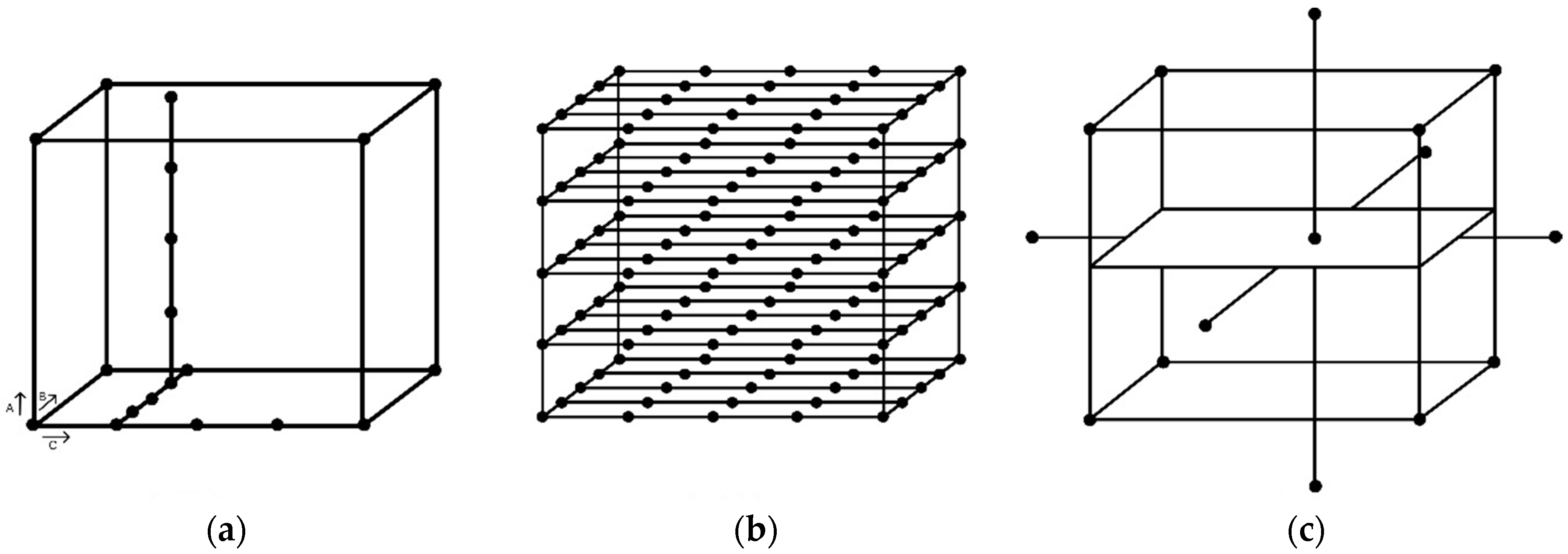
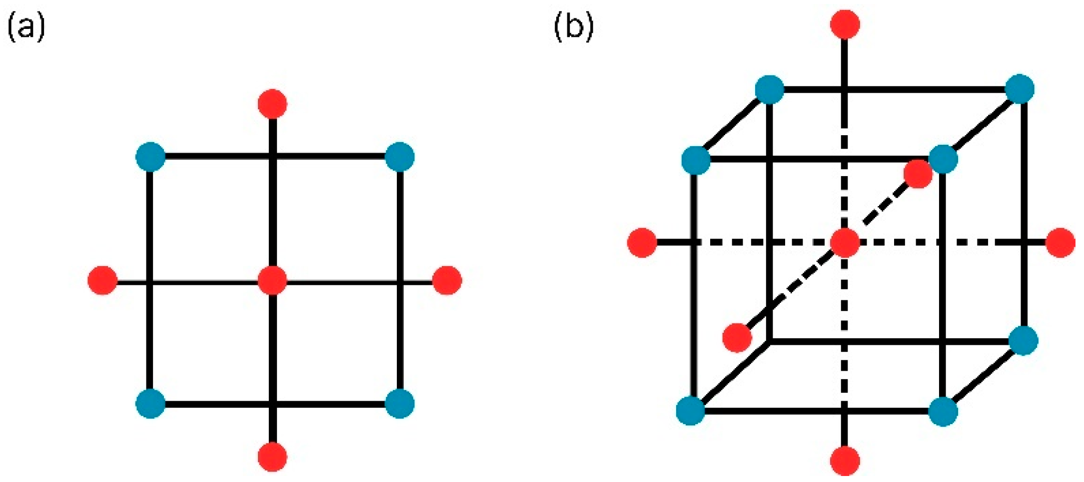
2.3. Central Composite Design

CCD is the most appropriate experimental design to fit the complete second-order polynomial model to experimental data. Introduced by Box and Wilson in 1951, it is a construction formed by three parts, namely (1) a factorial one, in which the independent variables are studied in two levels (2^k), low ($x_i=-1$) and high ($x_i=+1$), for all $i=1,\dots , k$, (2) 2k axial (or star) points, with all coordinates null but one, which corresponds to a value α (where, $\alpha =\sqrt[4]{2^k}$), or $-\alpha$, and (3) the central point ($x_1=\dots =x_k=0$), which must be replicated at least three times for pure error estimation purposes. Therefore, the design assumes a circular shape when k = 2 (Figure 2a), a spherical one when k = 3 (Figure 2b), and a hyperspherical one when k > 3 [25,33].

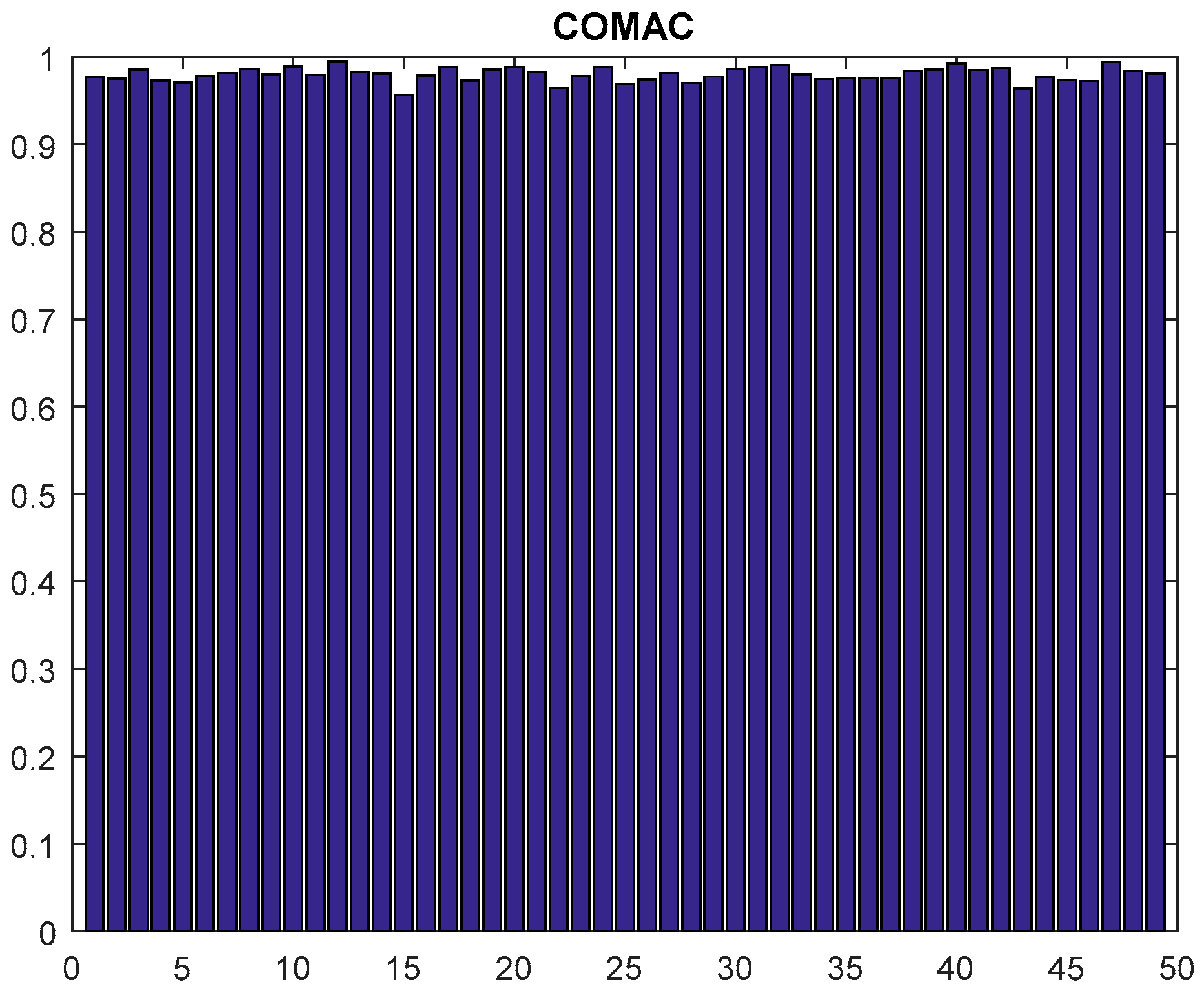
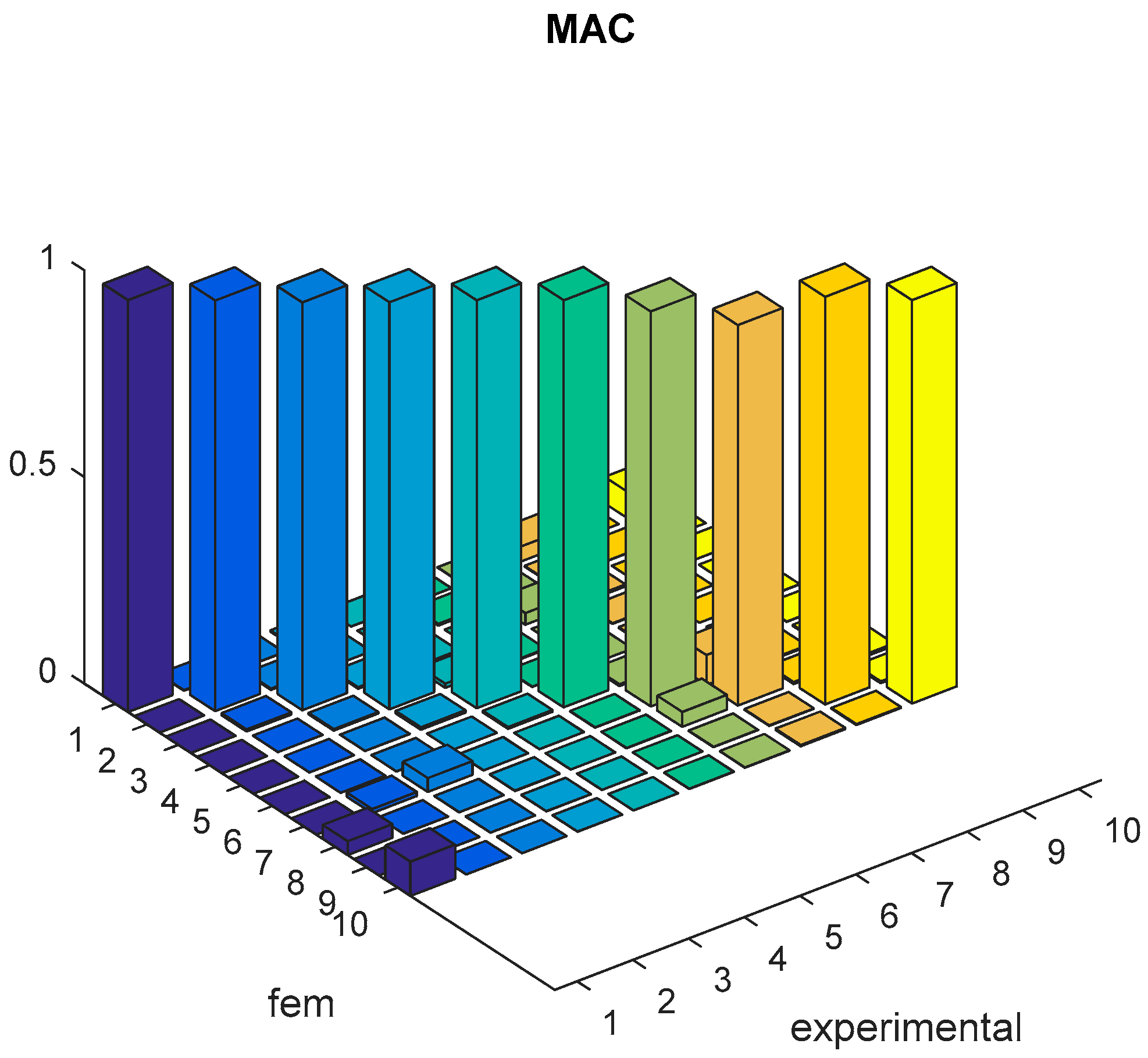
2.4. Correlation between Modal Models

The computational methodology in finite elements requires experimental data to fit the models and validate the solution. The main tool that provides such data is the experimental modal analysis (EMA). It identifies the modal parameters of a real structure (natural frequencies, vibration modes, and damping) from the structure’s vibration responses, when subjected to external force. Regarding the proposed experiment, the method was applied in the frequency domain to frequency response functions (FRF) obtained by the processing of both excitation (force) and response (structure acceleration) signals acquired experimentally by the single input single output (SISO) technique, according to which a power signal (input) and a response signal (output) were collected simultaneously by the acquisition module. A vibration exciter (shaker) was used for the force signal with a load cell applied at point 49 on the plate (see Figures 4 and 5a), whereas the response signal location varied at all points demarcated.

Data on the experimental modal analysis are always treated by specific algorithms that extract the modal parameters. When many similar pieces or assemblies are evaluated, the number of modes can be large enough to hamper the evaluation of the results. In this case, the modal assurance criterion (MAC) is the main criterion used. It provides a measurement of the consistency (degree of linearity) between estimates of a modal vector and an additional confidence factor in the evaluation of modal vectors extracted from either different excitation locations (reference), or different estimation algorithms of the modal parameters.

On the other hand, when two methods are to be compared (e.g., a numerical modal analysis and an experimental one) through the correlation between their vibration modes for the validation and calibration of a numerical model, an appropriate approach corresponds to the comparison of experimental modal forms with numerical modal ones. In this sense, the MAC becomes an indispensable tool for such a validation, and its coefficient is obtained by Equation (4).

$${\mathrm{MAC}}_{\left(i,j\right)}=\frac{{\left|{\left\{{\varphi }_i^r\right\}}^T\left\{{\varphi }_j^c\right\}\right|}^2}{({\left\{{\varphi }_i^r\right\}}^T\left\{{\varphi }_i^r\right\})\left({\left\{{\varphi }_j^c\right\}}^T\left\{{\varphi }_j^c\right\}\right)}$$

(4)

where

• $\left\{{\varphi }_i^r\right\}$ is the modal vector of the ith mode reference model;
• $\left\{{\varphi }_j^c\right\}$ is the modal vector of the jth mode calculated model.

The coefficient correlates the pairs of modal vectors, and its value ranges between 0 and 1. A coefficient equal to 1 indicates the modal vectors are identical and have a good correlation, whereas a 0 coefficient indicates they are orthogonal to each other, with no correlation.

However, a spatial dependence of the correlation parameters is observed in relation to the function of each degree of freedom (DF) individually called COMAC (coordinate modal assurance criterion). Woo and Vacca [21] correlated the degrees of freedom contained in two modal vectors, where one of them was the reference condition. COMAC indicates the contribution of each degree of freedom to the MAC values. Both COMAC and MAC values vary from 0 to 1, according to Equation (5).

$${\mathrm{COMAC}}_{\left(j\right)}=\frac{{\left({{\displaystyle \sum }}_{i=1}^n{\left\{{\varphi }_i^r\right\}}_j{\left\{{\varphi }_i^c\right\}}_j\right)}^2}{\left({{\displaystyle \sum }}_{i=1}^n{\left\{{\varphi }_i^r\right\}}_j{\left\{{\varphi }_i^r\right\}}_j\right)\left({{\displaystyle \sum }}_{i=1}^n{\left\{{\varphi }_i^c\right\}}_j{\left\{{\varphi }_i^c\right\}}_j\right)}$$

(5)

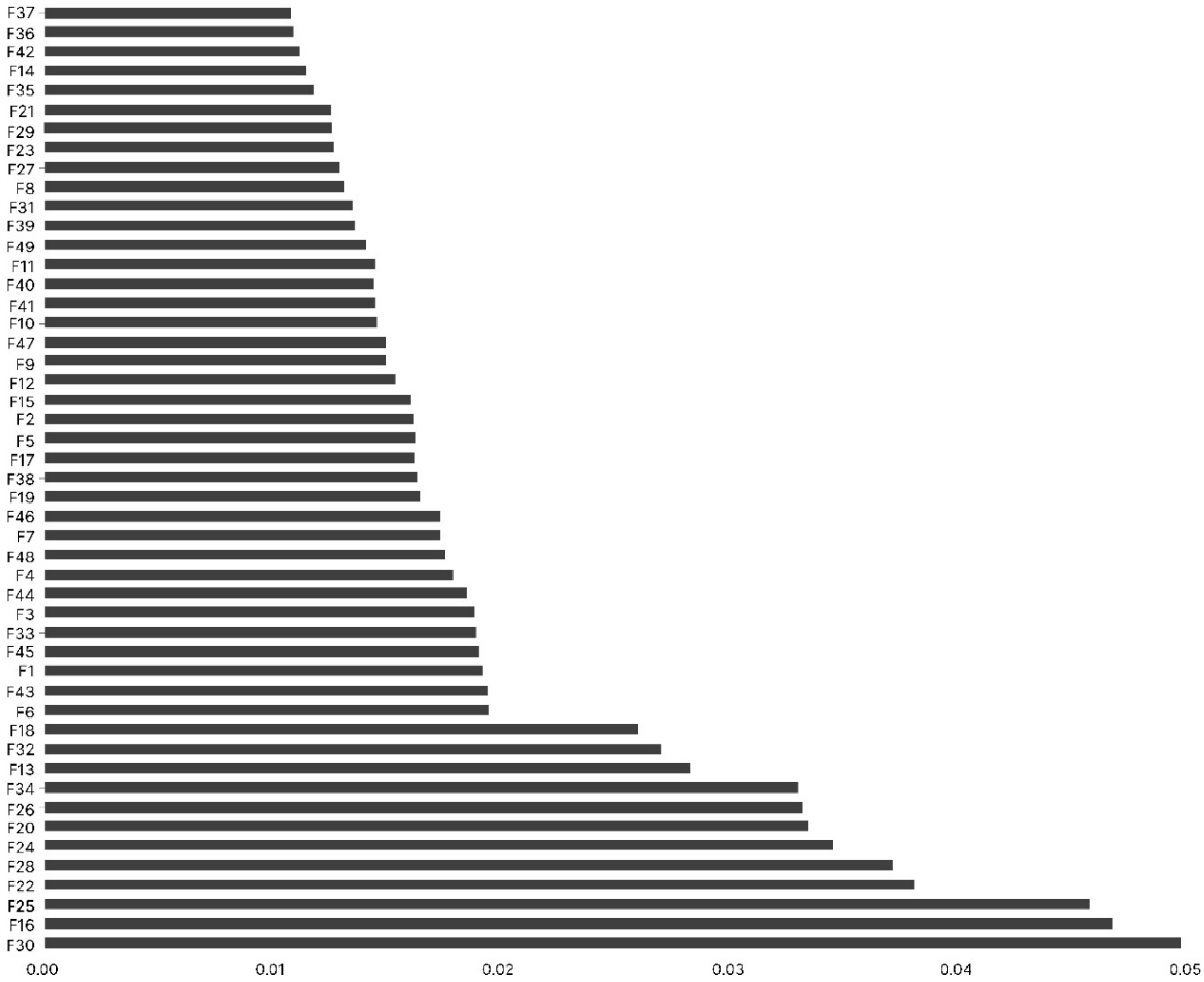
2.5. Random Forest Regressor

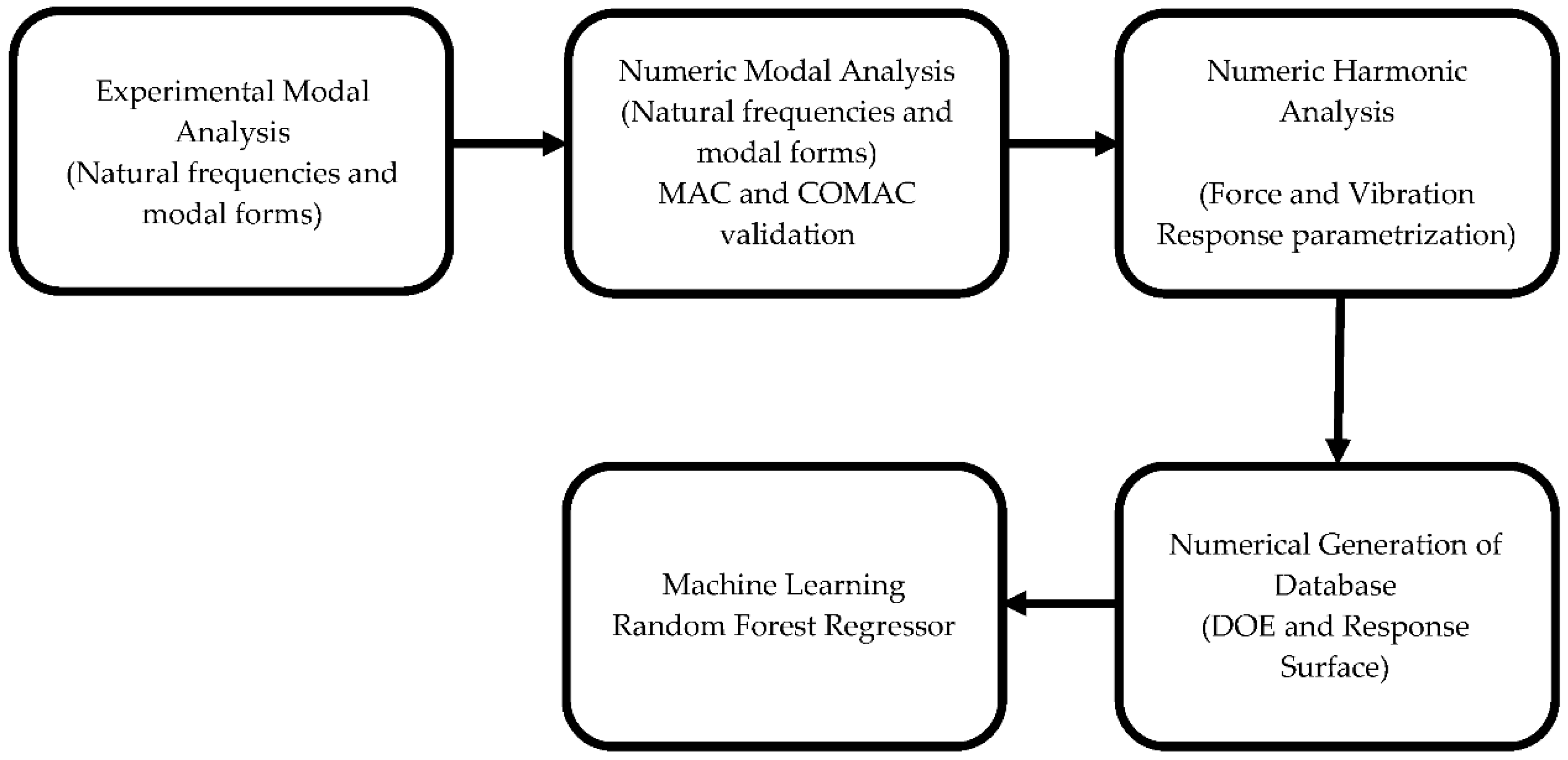
Random forests are a combination of decision tree classifiers such that each tree depends on the values of an independently sampled vector with the same distribution for all trees in the forest [17].

A random vector ${\Theta }_k$ is generated for the kth tree independently of the previous random vectors ${\Theta }_1, \dots , {\Theta }_{k-1}$, but with the same distribution. A tree is grown by a training set and ${\Theta }_k$, resulting in a classifier $h\left(x,{\Theta }_k\right)$, where x is an input vector. In a random selection of division, $\Theta$ consists of a number of independent random integers between 1 and k, and the nature and dimensionality of $\Theta$ depend on its use in building trees. After many trees have been generated, the most popular class is voted. According to [17,19], such a procedure is called a random forest. The accuracy of a random forest is primarily related to its convergence. In this sense, given a set of classifiers $h_1\left(X\right), h_2\left(X\right),\dots , h_k\left(X\right)$ and with the training set randomly presented from the distribution of the random vector Y, X, the margin function is defined by Equation (6).

$$mg\left(X,Y\right)=a{v}_{k}I\left(h_k\left(X\right)=Y\right)-ma{x}_{j \ne Y}a{v}_{k}I\left(h_k\left(X\right)=j\right)$$

(6)

where $I(·)$ is the indicator function. The margin measures the extent to which the average number of votes X, Y for the right class exceeds the average vote for any other class—the larger the margin, the more confident the rating. The generalization error is given by Equation (7) [12]:

$$P{E}^{*}=P_{X, Y}(mg \left(X,Y\right)<0)$$

(7)

where subscripts P_X,Y indicate the probability is above space X, Y.

The strong law of large numbers [22] is applied for a large number of trees in random forests and when the variables are independent, random, and identically distributed with a finite mean and the existence of a fourth central moment, the following theorem is established from the tree structure:

Theorem 1.

As the number of trees increases, for almost all sequences (${\Theta }_1, \dots$), $P{E}^{*}$converges to:

$$P_{X, Y}(P_{\Theta }\left(h\left(X,\Theta \right)=Y\right)-ma{x}_{j\ne Y}{P}_{\Theta }\left(h\left(X,\Theta \right)=j\right)<0)$$

(8)

According to Leo Breiman [12], Equation (8) explains why random forests do not adjust excessively as more trees are added, but produce a threshold value of the generalization error. A random forest regressor is formed by growing trees, depending on a random vector $\Theta$ such that the tree predictor $h\left(X,\Theta \right)$ assumes numerical values as opposed to class labels. The output values are numeric, and the training set is extracted independently of the vector distribution X, Y. The root-mean-square generalization error for any numerical predictor h(X) is presented in Equation (9).

$$E_{X, Y}\left(Y-h\left(X^2\right)\right)$$

(9)

3. Methodology

Figure 3 displays a diagram of the methodology used for the identification of the excitation force at the expense of vibration, which creates a regressor model via a random forest from a dataset generated by the response surface. Each step will be detailed in Section 3.1, Section 3.2, Section 3.3 and Section 3.4.

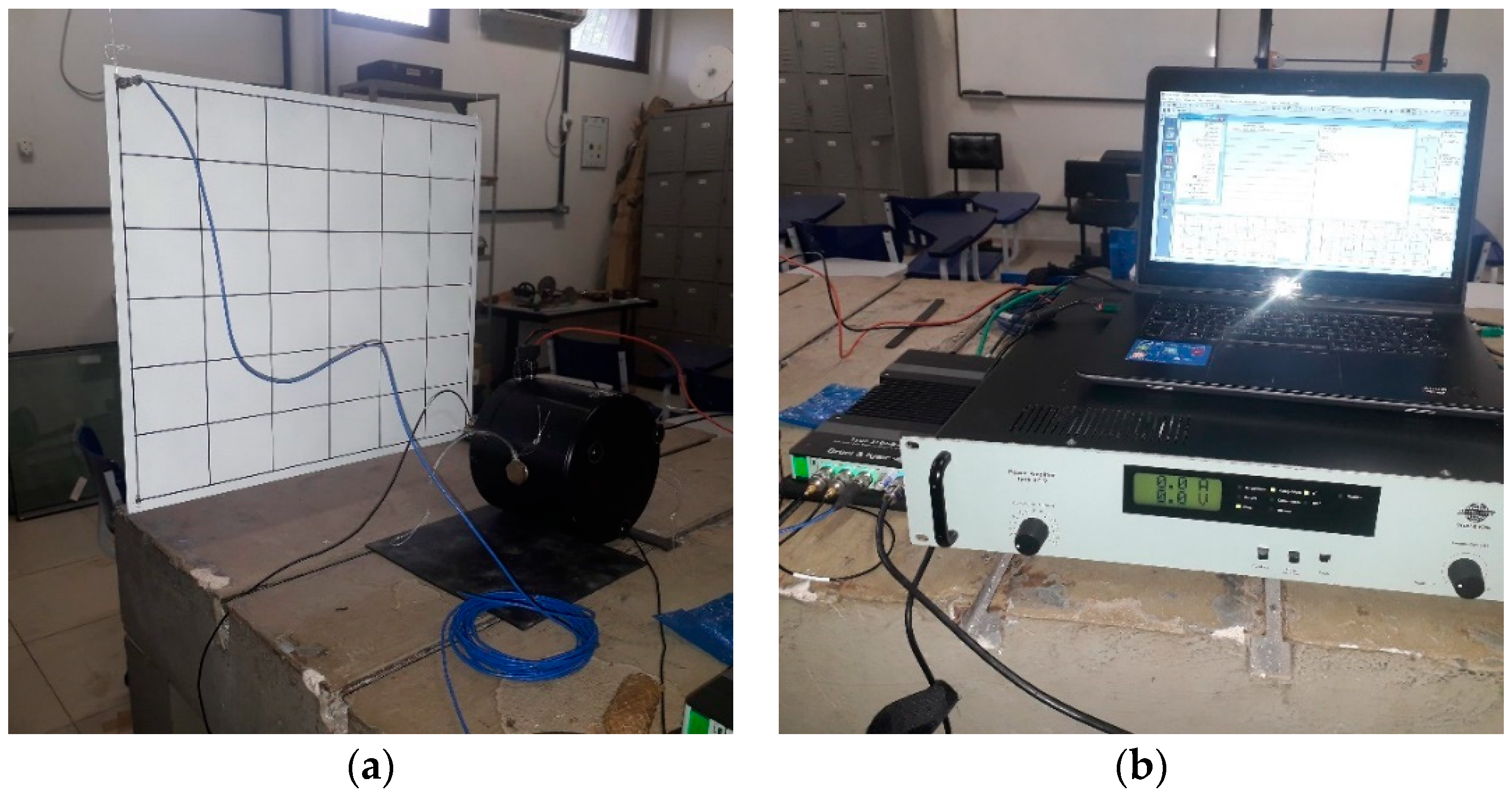
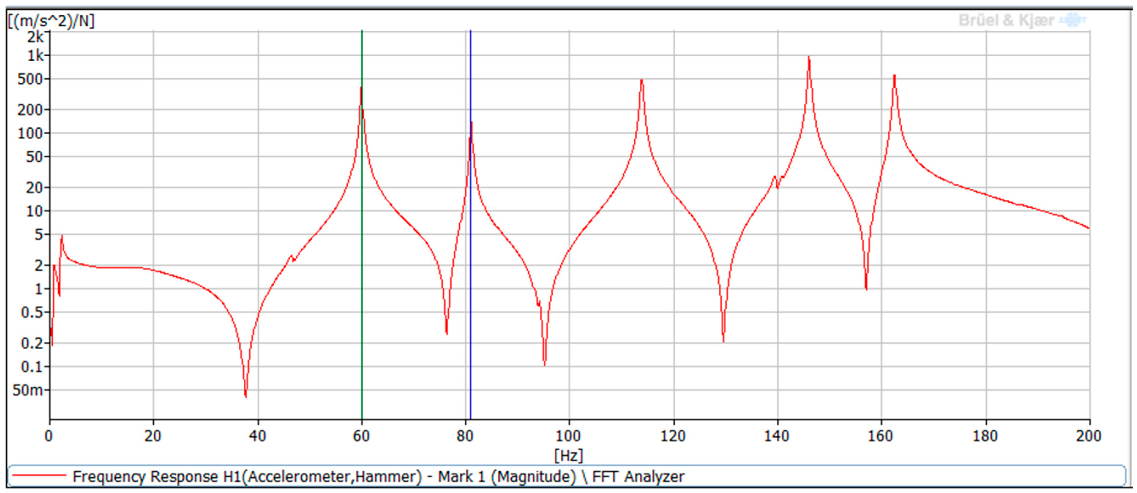
3.1. Experimental Modal Analysis

A plate of 420 mm × 360 mm dimensions and 3 mm thickness suspended by nylon threads simulated a free-free condition, arbitrarily discretized at 49 points, as shown in Figure 4a. The mesh created had a 10 mm offset from the edges of the sheet and each point was spaced 66.2 mm and 56.7 mm from the other point horizontally and vertically, respectively. Point 49 was chosen for the application of the excitation force (Figure 4a), since it can excite a greater number of modes [2]. The accelerometer was fixed at each intersection of the horizontal and vertical lines at locations 1 to 49, its fixation was changed with each measurement, following the numerical sequence in Figure 5a. Figure 4b displays the acquisition system with a signal analyzer, a computer, and an amplifier.

The 49 points were established on the front of the plate, from left to right and from top to bottom (see Figure 5a), for the vibration measurement. Point 49, located on the lower right, was chosen for the fixation of the force sensor (load cell) and insertion of the excitation force, since it excites a greater number of plate modes. The direction of both excitation and responses was perpendicular to the plate surface. Figure 4a shows the position of the vibration exciter (shaker) fixed to the plate at point 49 and the accelerometer fixed at point 1 for the vibration measurement.

Figure 4b displays the measurement system consisting of an accelerometer (PCP 353B16), a force sensor (B&K 8001), load cell type, a vibration exciter (B&K 4809), a signal amplifier (B&K 2716), a signal analyzer (B&K 3160-B-042) with Pulse Labshop software, and a notebook. The values of the natural frequencies were used for the validation of the model described in Section 3.2.

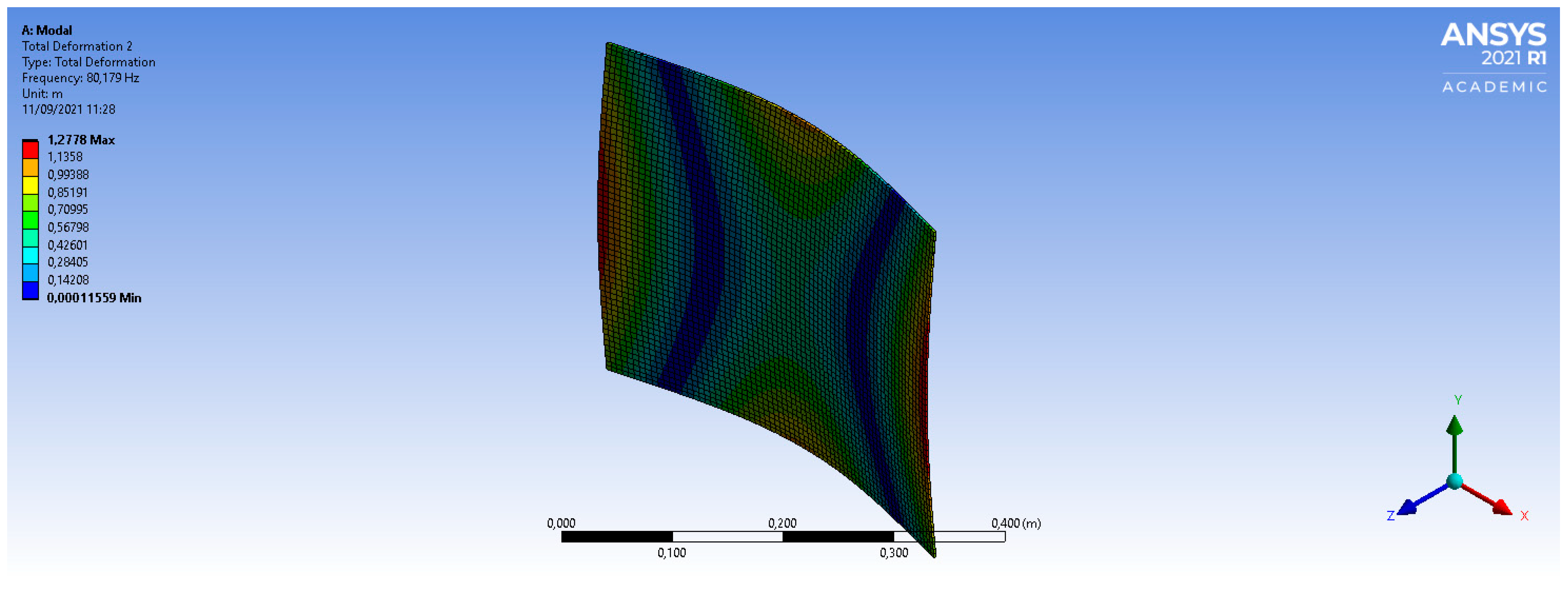
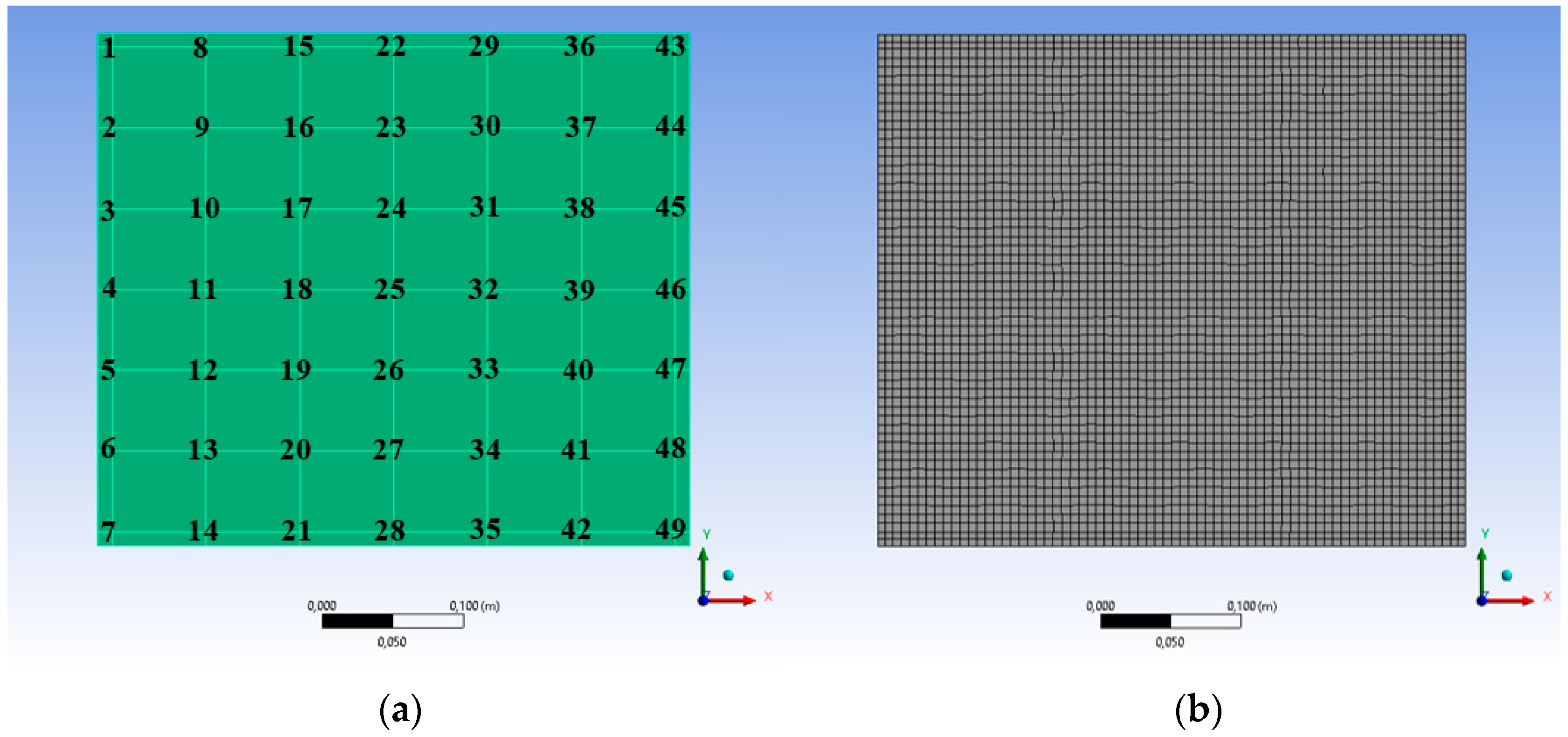
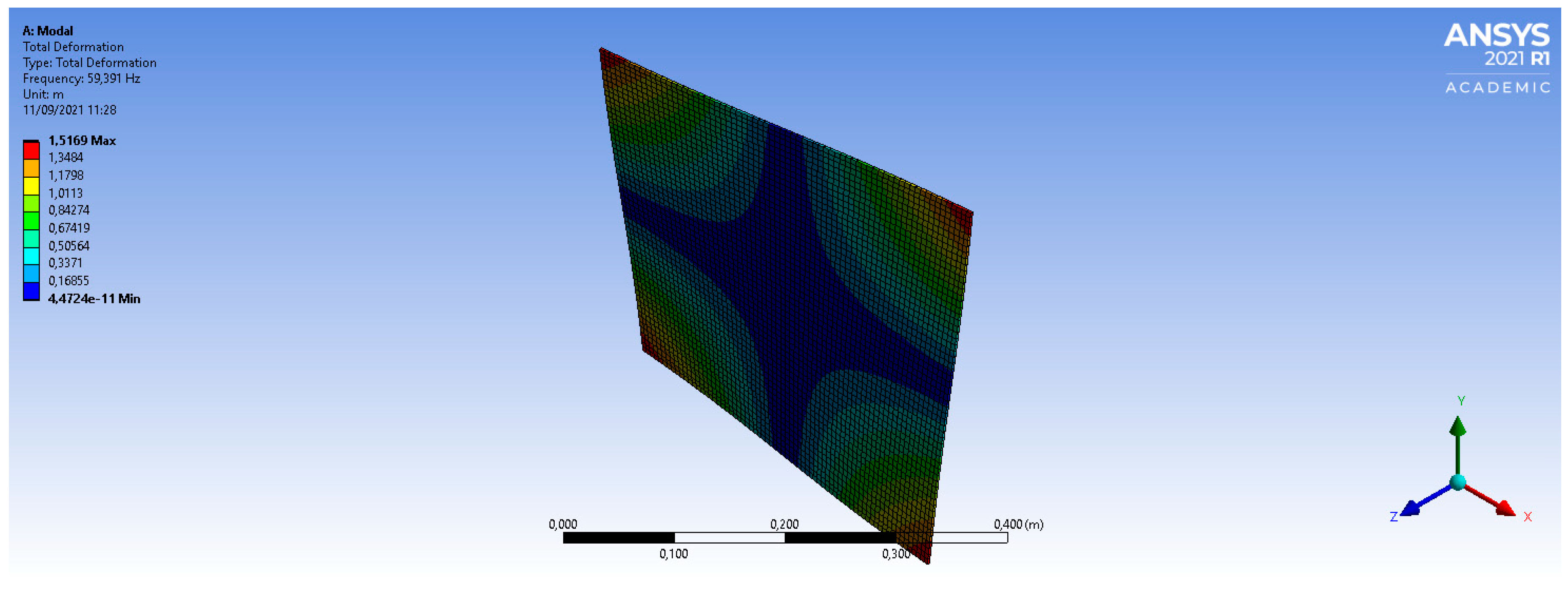
3.2. Numerical Modal Analysis

The material properties used in the numerical model, namely 207 GPa for Young’s modulus and 7800 kg/m³ for the specific mass—both properties of steel—were used for the creation of the numerical model of the sheet. A numerical modal analysis was conducted through the finite element method and the use of Ansys Mechanical Academics software. The material with the same specifications as the steel plate and boundary conditions for the free-free model was used in the preprocessing stage, whereas in the processing step, a plate element was employed and the block Lanczos method was adopted for the modal extraction. The modal superposition model was used for the extraction of the modes; the modal forms were expanded and used in the harmonic analyses described in the next section. Figure 5a depicts the model geometry for the maintenance of the discretization used experimentally in the sheet, and Figure 5b displays its structured mesh with 4060 elements and 4129 nodes.

3.3. Numerical Harmonic Analysis

Harmonic analyses were performed in the numerical modal model and validated by the experimental modal analysis. The z-direction component of the force perpendicular to the model plane (see Figure 5), the force frequency, and the average value of the z-direction component of the acceleration were parameterized. The value of the acceleration amplitude was calculated for each force fixation point, in each of the 49 points of the model and RSM was further applied. The force amplitude was varied with a 0.1 mN step, from 0.1 mN to 5 mN, and the force frequency was varied with a 5 Hz step, from 5 Hz to 250 Hz, for each amplitude value.

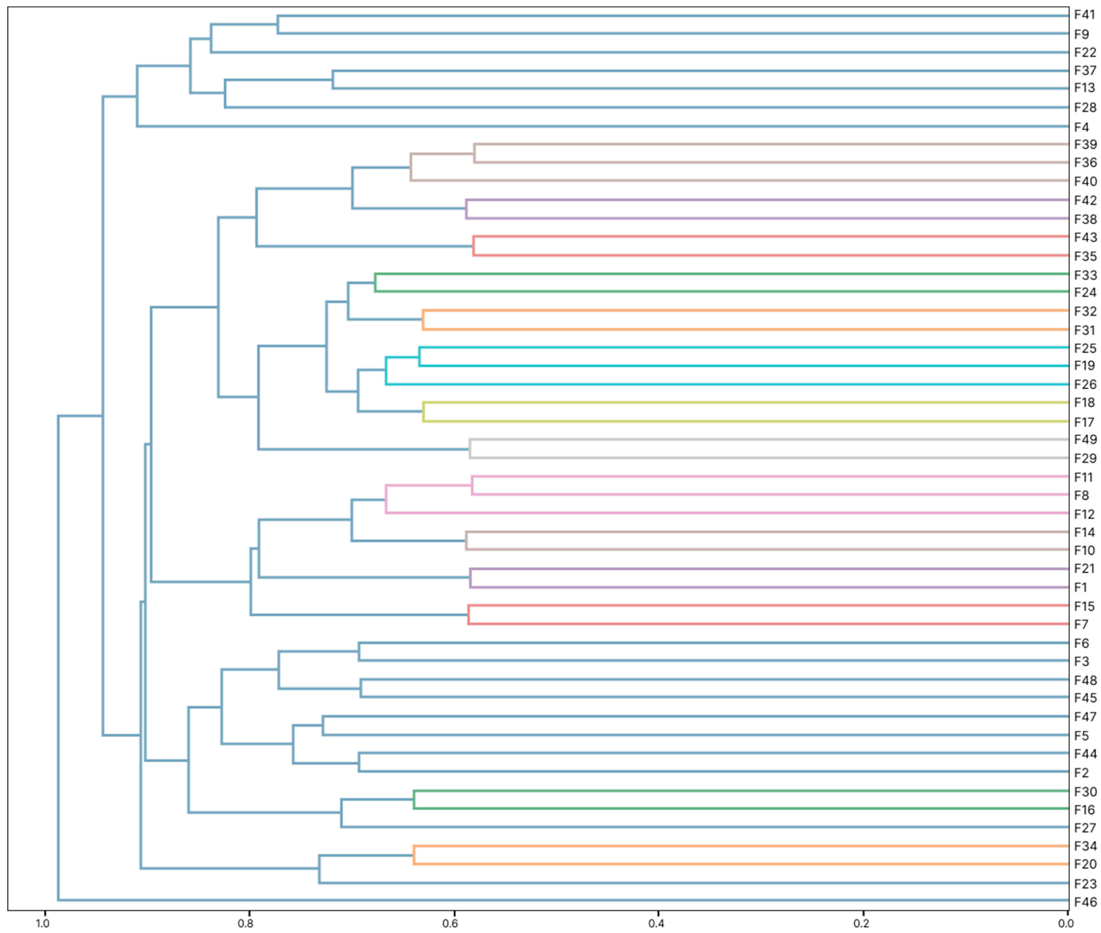
3.4. Machine Learning Random Forest Regressor

The machine learning model adopted was a random forest regressor, which aims to recognize a pattern in a data set to be used in the prediction of the excitation strength. A regression model was used due to the continuous variables in the data. Initially, 80% of the data were randomly separated for training the random forest regressor and the other 20% were randomly reserved for its testing, according to the methodology presented in [17].

The database generated by the RSM used for training and validating the RFR model had 122,500 lines and 53 columns, with 49 features (vibration responses) and 4 classes (amplitude, frequency, position in the x coordinate, and position in the y coordinate of the forces).

The degree of importance of the features in the prediction of the model was previously analyzed by RFR to help reduce their number. The correlation between the remaining features was then evaluated with the use of Spearman’s correlation [34]. The Spearman dendrogram shows the features in the ordinate and the abscissa axis represents the Spearman Index, which ranges from 0 to 1—the closer the index to 1, the lower the correlation between the features and their groups, hence, the greater the correlation between the features, the more redundant their information for the mode (in this case, one of them can be excluded without harming the model’s accuracy).

The Python language code used for both data processing and RFR application is available at https://github.com/FabioSetubal/forceidentification (accessed on 22 April 2022).

4. Results and Discussions

The experimental modal analysis that validated the FEM model identified natural frequencies of some free-free plate vibration modes. Figure 6 shows a typical point frequency response function (FRF) of inertance measured at point 49 and characterized by its antiresonances (decreasing peaks).

The two cursors mark the first two natural bending frequencies of the plate obtained experimentally. Frequency values of 60.0 Hz and 81.0 Hz were used for the FEM calibration. Two peaks referring to rigid body vibration modes can be observed close to zero hertz, since the structure was tested in a free-free condition. Other natural frequencies of the plate related to other vibration modes can be observed above 81.0 Hz.

Figure 7 and Figure 8 show the results of the numerical modal analysis for the first two bending modes. They were obtained after adjustments in the model according to the experimental modal results. Curvatures of the modal forms can be observed for each natural frequency, and Figure 7 displays the first bending mode at the natural frequency of 59.4 Hz, which is close to the 60.0 Hz value obtained in the experimental modal analysis.

Figure 8 depicts the second bending mode with a natural frequency of 80.2 Hz, which is close to the 81.0 Hz natural frequency obtained experimentally.

Figure 9 and Figure 10, respectively, show comparisons of natural frequencies and modal forms conducted by MAC and COMAC for the first 10 modes. The choice of the number of modes to be studied depends on the type of problem; in this study, only the first two modes were analyzed.

According to the MAC values, the diagonal modes are close to unity, indicating a good correlation between them. Therefore, COMAC also shows a good correlation between the degrees of freedom (GDL) of the modes, indicated by levels close to one (Figure 10).

Since the random forest model internally calculates a feature importance ranking in its algorithm, the greater the error reduction in decision splits made according to a given feature in each decision tree, the more important the variable. In this study, the features analyzed were the acceleration responses at each of the 49 points, for each step and position of the excitation force in the model. Figure 11 shows the graph of the percentage importance of the features and their position in the model regarding the best prediction of force by the RFR model.

According to Figure 11, the feature at position 37 (F37), i.e., the first position from top to bottom, contributes approximately 1% to the model prediction, and the feature at point 30 (F30), i.e., first position from bottom to top, shows a 5% importance in the model prediction, thus being the most important variable in the prediction.

Figure 12 displays the Spearman’s dendrogram for the 49 variables. All variables show a small correlation, since their information begins to match when Spearman’s indices are close to 60%, indicating neither significant redundancy of information, nor the exclusion of the features from the analysis.

After the importance of the features were analyzed (Figure 11), possible redundancies of information in the 49 features were investigated. According to Figure 12, the features have low correlation and, therefore, do not provide redundant information in the model. However, their number could be reduced with no significant loss in the performance metrics of the model (see the degree of importance in Figure 11).

In the RFR methodology, each tree in the forest uses samples from the database randomly, returning them (or not) to the database. The comparison of the prediction metrics among the 49 initial measurement points and the comparison with reductions to 24 and 12 points in

Table 1. Comparison of prediction metrics among the initial 49 measurement points and their reductions to 24 and 12 measurement points.

Time: 3 min 56 s—With 49 Measurement Points			Time: 1 min 38 s—Reduction to 24 Measurement Points			Time: 56.1 s—Reduction to 12 Measurement Points
	MAE	R2		MAE	R2		MAE	R2
Training	0.034146	0.999749	Training	0.039241	0.999733	Training	0.055990	0.999635
Test	0.085874	0.998355	Test	0.096125	0.998335	Test	0.145074	0.997431
OOB (Test)	0.092646	0.998172	OOB (Test)	0.106599	0.998049	OOB (Test)	0.151995	0.997316

show the efficiency of the model remained excellent, despite the reduction of points, thus guaranteeing, in practice, a reduction in the measurement time, due to both reduction and choice of the best location for future vibration measurements. Moreover, in case of no replacement of samples, the mean absolute error (MAE) for the 49 measurement points maintained their values between 3% and 5% in comparison with those after the reduction of measurement points to 24 and 12, keeping an accuracy above 99% in all three cases.

Considering sample replacement, the random forest uses a parameter inherent to the execution process of its algorithm, called the out-of-bag (OOB) cross-validation method or method with replacement. Each decision tree in the forest uses a random sample from the database and returns it to the database, obtaining a random and independent error between one sample and another, until all samples have been used. Consequently, RFR obtains an average error of all independent errors of each tree and displays it through the OOB. Table 1 shows the MAE and accuracy (R²) values obtained for both training and test data for each case of number of features with no sample replacement, as well as the MAE and R² of the respective value of OOB, used in the sample replacement process, applied in the test step in the RFR model.

5. Conclusions

This article presented the results from the application of a method that, based on machine learning, used the response surface method and a random forest regression to identify forces in a FEM model of structures.

The methodology was tested with the use of a database generated by computer simulation and the application of FEM, RSM, and RFR, which was divided into two parts, namely training and model testing. According to the results, the model was able to predict the amplitude, frequency, and location of forces accurately and quickly, obtaining an accuracy greater than 99%.

The analyses with variable parameters revealed the feature reduction method proved efficient, reducing specific measurement points from 49 to 12, with a 99% accuracy. The reduction process enabled the identification of the most important locations for vibration measurements, thus reducing computational time.

The RFR application with no sample replacement to each tree provided smaller errors and a better accuracy in comparison with its procedure with the replacement of the samples. The replacement method procedure was demonstrated through the MAE and R² values for the OOB, which proved less efficient.

A limitation of the research refers to the need for a validated modal numerical model of the structure so that numerical forces can be applied to train the predictor regression model. On the other hand, ill-conditioning problems found in traditional inverse problem-solving methods are avoided.

A support tool based on machine learning was implemented and can be directly integrated to the areas of electrical, civil, and mechanical engineering, ensuring a considerable increase in the reliability of structural projects of electrical power equipment such as transformers, railway projects, civilians, and mechanics.

References

1. Rezayat, A.; Nassiri, V.; de Pauw, B.; Ertveldt, J.; Vanlanduit, S.; Guillaume, P. Identification of Dynamic Forces Using Group-Sparsity in Frequency Domain. Mech. Syst. Signal Processing 2016, 70–71, 756–768. [Google Scholar] [CrossRef]
2. Feng, W.; Li, Q.; Lu, Q. Force Localization and Reconstruction Based on a Novel Sparse Kalman Filter. Mech. Syst. Signal Processing 2020, 144, 106890. [Google Scholar] [CrossRef]
3. Lin, T.-K.; Liang, J.-C.; Zhou, G.-D.; Yi, T.-H.; Xie, M.-X.; Ciang, C.C.; Lee, J.-R.; Bang, H.-J. Structural Health Monitoring for a Wind Turbine System: A Review of Damage Detection Methods. Meas. Sci. Technol. 2008, 19, 122001. [Google Scholar] [CrossRef] [Green Version]
4. Zhang, F.; Ji, S.; Shi, Y.; Zhan, C.; Zhu, L. Investigation on Vibration Source and Transmission Characteristics in Power Transformers. Appl. Acoust. 2019, 151, 99–112. [Google Scholar] [CrossRef]
5. Altstadt, E.; Scheffler, M.; Weiss, F.P. Component Vibration of VVER-Reactors—Diagnostics and Modelling. Prog. Nucl. Energy 1995, 29, 129–138. [Google Scholar] [CrossRef]
6. Qiao, B.; Chen, X.; Luo, X.; Xue, X. A Novel Method for Force Identification Based on the Discrete Cosine Transform. J. Vib. Acoust. Trans. ASME 2015, 137, 051012. [Google Scholar] [CrossRef]
7. Feng, W.; Li, Q.; Lu, Q.; Wang, B.; Li, C. Time Domain Force Localization and Reconstruction Based on Hierarchical Bayesian Method. J. Sound Vib. 2020, 472, 115222. [Google Scholar] [CrossRef]
8. Goutaudier, D.; Gendre, D.; Kehr-Candille, V.; Ohayon, R. Single-Sensor Approach for Impact Localization and Force Reconstruction by Using Discriminating Vibration Modes. Mech. Syst. Signal Processing 2020, 138, 106534. [Google Scholar] [CrossRef]
9. Lu, Z.R.; Law, S.S. Force Identification Based on Sensitivity in Time Domain. J. Eng. Mech. 2006, 132, 1050–1056. [Google Scholar] [CrossRef]
10. Maia, N.M.M.; Lage, Y.E.; Neves, M.M. Recent Advances on Force Identification in Structural Dynamics. Adv. Vib. Eng. Struct. Dyn. 2012, 1, 103–132. [Google Scholar] [CrossRef] [Green Version]
11. Yang, Y.; Gong, N.; Xie, K.; Liu, Q. Predicting Gasoline Vehicle Fuel Consumption in Energy and Environmental Impact Based on Machine Learning and Multidimensional Big Data. Energies 2022, 15, 1602. [Google Scholar] [CrossRef]
12. Barbaresi, A.; Ceccarelli, M.; Menichetti, G.; Torreggiani, D.; Tassinari, P.; Bovo, M. Application of Machine Learning Models for Fast and Accurate Predictions of Building Energy Need. Energies 2022, 15, 1266. [Google Scholar] [CrossRef]
13. Bhushan, S.; Burgreen, G.W.; Brewer, W.; Dettwiller, I.D. Development and Validation of a Machine Learned Turbulence Model. Energy 2021, 14, 1465. [Google Scholar] [CrossRef]
14. Almasi, S.; Ghobadian, B.; Najafi, G.H.; Yusaf, T.; Soufi, M.D.; Hoseini, S.S. Optimization of an Ultrasonic-Assisted Biodiesel Production Process from One Genotype of Rapeseed (Teri (OE) R-983) as a Novel Feedstock Using Response Surface Methodology. Energy 2019, 12, 2656. [Google Scholar] [CrossRef] [Green Version]
15. Anguebes-Franseschi, F.; Abatal, M.; Bassam, A.; Soberanis, M.A.E.; Tzuc, O.M.; Bucio-Galindo, L.; Quiroz, A.V.C.; Ucan, C.A.A.; Ramirez-Elias, M.A. Esterification Optimization of Crude African Palm Olein Using Response Surface Methodology and Heterogeneous Acid Catalysis. Energy 2018, 11, 157. [Google Scholar] [CrossRef] [Green Version]
16. Dang, S.; Peng, L.; Zhao, J.; Li, J.; Kong, Z. A Quantile Regression Random Forest-Based Short-Term Load Probabilistic Forecasting Method. Energy 2022, 15, 663. [Google Scholar] [CrossRef]
17. Leo Breiman 17-Random Forest 2001; University of California: Los Angeles, CA, USA, 2001; pp. 1–33.
18. Segal, M.R. Machine Learning Benchmarks and Random Forest Regression. UCSF Recent Work Title. 2003. Available online: https://escholarship.org/uc/item/35x3v9t4 (accessed on 7 March 2022).
19. Johansson, U.; Boström, H.; Löfström, T.; Linusson, H. Regression Conformal Prediction with Random Forests. In Proceedings of the Machine Learning; Kluwer Academic Publishers: Norwell, MA, USA, 2014; Volume 97, pp. 155–176. [Google Scholar]
20. Randall, J. Allemang 14-The Modal Assurance Criterion Twenty Years of Use and Abuse. Sound Vib. 2003, 37, 14–21. [Google Scholar]
21. Woo, S.; Vacca, A. An Investigation of the Vibration Modes of an External Gear Pump through Experiments and Numerical Modeling. Energy 2022, 15, 796. [Google Scholar] [CrossRef]
22. Henkel, M.; Weijtjens, W.; Devriendt, C. Fatigue Stress Estimation for Submerged and Sub-Soil Welds of Offshore Wind Turbines on Monopiles Using Modal Expansion. Energy 2021, 14, 7576. [Google Scholar] [CrossRef]
23. Dziedziech, K.; Mendrok, K.; Kurowski, P.; Barszcz, T. Multi-Variant Modal Analysis Approach for Large Industrial Machine. Energies 2022, 15, 1871. [Google Scholar] [CrossRef]
24. Najafi, B.; Ardabili, S.F.; Mosavi, A.; Shamshirband, S.; Rabczuk, T. An Intelligent Artificial Neural Network-Response Surface Methodology Method for Accessing the Optimum Biodiesel and Diesel Fuel Blending Conditions in a Diesel Engine from the Viewpoint of Exergy and Energy Analysis. Energy 2018, 11, 860. [Google Scholar] [CrossRef] [Green Version]
25. Box, G.E.P.; Wilson, K.B. On the Experimental Attainment of Optimum Conditions. J. R. Stat. Soc. Ser. B (Methodol.) 1951, 13, 1–38. [Google Scholar] [CrossRef]
26. Haaland, P.D. Experimental Design in Biotechnology; CRC Press: Boca Raton, FL, USA, 2020. [Google Scholar] [CrossRef]
27. Jo, S.T.; Shin, H.S.; Lee, Y.G.; Lee, J.H.; Choi, J.Y. Optimal Design of a BLDC Motor Considering Three-Dimensional Structures Using the Response Surface Methodology. Energy 2022, 15, 461. [Google Scholar] [CrossRef]
28. Costarrosa, L.; Leiva-Candia, D.E.; Cubero-Atienza, A.J.; Ruiz, J.J.; Dorado, M.P. Optimization of the Transesterification of Waste Cooking Oil with Mg-al Hydrotalcite Using Response Surface Methodology. Energy 2018, 11, 302. [Google Scholar] [CrossRef] [Green Version]
29. Kaneko, S.; Tomigashi, A.; Ishihara, T.; Shrestha, G.; Yoshioka, M.; Uchida, Y. Proposal for a Method Predicting Suitable Areas for Installation of Ground-Source Heat Pump Systems Based on Response Surface Methodology. Energy 2020, 13, 1872. [Google Scholar] [CrossRef] [Green Version]
30. Abdullah, M.F.; Zulkifli, R.; Moria, H.; Najm, A.S.; Harun, Z.; Abdullah, S.; Ghopa, W.A.W.; Sulaiman, N.H. Assessment of Tio2 Nanoconcentration and Twin Impingement Jet of Heat Transfer Enhancement—A Statistical Approach Using Response Surface Methodology. Energy 2021, 14, 595. [Google Scholar] [CrossRef]
31. Beebe, K.R.; Pell, R.J.; Seasholtz, M.B.; Download Beebe, K.R.; Pell, R.J.; Seasholtz, M.B. Chemometrics: A Practical Guide [PDF]–Sciarium. Available online: https://sciarium.com/file/376960/ (accessed on 7 March 2022).
32. Zhao, Z.; Xu, L.; Gao, J.; Xi, L.; Ruan, Q.; Li, Y. Multi-Objective Optimization of Parameters of Channels with Staggered Frustum of a Cone Based on Response Surface Methodology. Energy 2022, 15, 1240. [Google Scholar] [CrossRef]
33. Benício de Barros Neto; Ieda Spacino Scarminio; Roy Edward Runs Como Fazer Experimentos 2aed Barros Scarminio Bruns OCR|PDF|Experimento|Estatísticas. Available online: https://pt.scribd.com/doc/153246515/Como-Fazer-Experimentos-2aEd-Barros-Scarminio-Bruns-OCR (accessed on 7 March 2022).
34. Shaikh, M.A.H.; Barbé, K. Wiener-Hammerstein System Identification: A Fast Approach Through Spearman Correlation. IEEE Trans. Instrum. Meas. 2019, 68, 1628–1636. [Google Scholar] [CrossRef]
Figure 1. Methodologies for an experimental procedure: (a) Univariate analysis; (b) matrix with all combinations; and (c) CCD.
Energies 15 03786 g001
Figure 2. Central Composite Design (CCD): (a) CCD for two factors (k = 2 and α = 2 ); (b) CCD for three factors (k = 3 and α = 3 ).
Energies 15 03786 g002
Figure 3. Flowchart of the fundamental steps taken for the achievement of the study objective.
Energies 15 03786 g003
Figure 4. Experimental system: (a) suspended plate with force and acceleration measurement points; (b) signal acquisition system.
Energies 15 03786 g004
Figure 5. Numerical model in FEM used in modal and harmonic analyses: (a) geometry with the locations of measurement points; (b) discretization.
Energies 15 03786 g005
Figure 6. Point frequency response function of the plate highlighting the first two natural frequencies.
Energies 15 03786 g006
Figure 7. First bending mode of the model at the natural frequency of 59.4 Hz.
Energies 15 03786 g007
Figure 8. Second bending mode of the model at the natural frequency of 80.2 Hz.
Energies 15 03786 g008
Figure 9. Graph with MAC values for the experimental and numerical models.
Energies 15 03786 g009
Figure 10. Graph with COMAC values used in the comparison of GDL of experimental and numerical modes.
Energies 15 03786 g010
Figure 11. Importance of the locations of vibration measurements (features), on the ordinate axis, and their respective percentage contributions, on the abscissa axis, in the RFR accuracy.
Energies 15 03786 g011
Figure 12. Spearman’s dendrogram with the correlation between the 49 variables.
Energies 15 03786 g012