A Novel Layered Slice Algorithm for Soil Heat Storage and Its Solving Performance Analysis

Abstract

According to the structural and heat transfer characteristics of soil heat storage, a novel layered slice algorithm is proposed to realize the rapid and accurate solution to the problem. The heat transfer process between the double U-tube heat exchanger and the surrounding soil is taken as an example to analyze its solving performance. The study finds that the layered slice algorithm has higher simulation precision and faster solving speed. Its maximum relative error of temperature is only 0.19%. Compared with the traditional 3D simulation algorithm, it can accelerate about 2.2~2.56 times. At the same time, the layered slice algorithm has an excellent parallel characteristic. Its maximum parallel speedup ratio is more than twice that of the traditional 3D algorithm. Due to the superior solving performance, the proposed algorithm can help the optimization design of the buried-tube heat exchangers.

1. Introduction

With the development of the social economy, people pay increasing attention to developing and utilizing new energy, especially solar energy. However, solar energy has intermittent and instability characteristics, leading to a mismatch between supply and demand. Therefore, heat storage must be adopted to solve the contradiction between supply and demand [1,2,3].

Conventional heat storage ways include water tank heat storage [4,5,6], aquifer heat storage [7,8,9], soil heat storage [10,11,12], gravel-water heat storage [13,14,15], and phase-change heat storage [16,17,18], etc. The soil heat storage has the advantages of low cost, high potential, and excellent environmental friendliness. Therefore, this type of heat storage has become the research focus in recent years. Guo et al. [19] established an unsteady theoretical model of solar chimney power generation considering soil heat storage. They researched the influence of different soil types on the system’s output power. The results showed that it is beneficial for the system to use the soils with high specific-heat capacity and thermal conductivity as heat-storage materials. Zhang et al. [20] studied a low-cost seasonal solar soil heat storage system for greenhouse heating. The heat-storage technology was utilized to reduce the greenhouse’s energy demand under extreme cold and consecutive cloudy conditions in winter.

The soil heat storage and the ground-source heat pump can be combined to use the same set of buried-pipe heat exchangers [21]. The combined system can address problems of soil thermal imbalance and improve the heat pump efficiency [22,23]. Therefore, different ground-source heat pump systems assisted with solar energy [24,25], industrial waste heat [26], or mixed heat source [27] have been widely studied and applied. Naranjo-Mendoza et al. [28] experimentally investigated a solar-assisted, ground-source heat pump system, which uses a set of shallow vertical boreholes to store heat underground seasonally. The research results show that the system can well meet the demand for building heating in winter. Solar energy stored underground can be used to restore the soil’s temperature and improve system efficiency. Cui et al. [29] proposed a novel buried-pipe heat exchanger with a vertical borehole for the seasonal storage of industrial waste heat. They studied the influence of some key parameters on its performance. A heating demonstration project [30] was recently built for urban heat supply in Inner Mongolia, China. The system maximally utilizes renewable energy and industrial waste heat through large-scale seasonal heat storage.

For the ground-source heat pump system assisted with soil heat storage, the experimental research, especially the demonstration research, has certain limitations. This type of research has the disadvantages of high investment costs and long experiment periods. In addition, generality is lacking for the experimental results. The data from some regions are difficult to apply to other areas. In recent years, the corresponding numerical simulation research has partially replaced the experimental and demonstration studies with the rapid development of computer technology. It reduces the research cost, shortens the research cycle, and plays an increasingly important role in engineering applications. The core of simulating the system is to calculate the process of heat -and mass-coupled transfer between the buried-pipe heat exchanger and the surrounding soil. However, it is difficult to accurately obtain the soil moisture content, porosity, groundwater velocity, and other parameters in the practical calculation process for heat storage. For overcoming the problem, the effective thermophysical properties are measured by thermal response testing [31,32] to replace the actual soil parameters. Then, the complex coupling process in the soil can be regarded as a single heat conduction problem. At present, based on the effective thermophysical properties, the linear source theory [33,34], the cylindrical source theory [35,36], and the three-dimensional (3D) numerical simulation method [37,38] can be used to calculate and investigate the variation laws of the temperature in the soil. However, in the first two approaches, it is hard to obtain soil temperature accurately. This issue can be solved by adopting the 3D numerical simulation method, but its calculation time is too long to meet actual engineering demand.

In order to obtain the change laws of soil temperature in the process of heat storage quickly and accurately, a layered slice algorithm is proposed by the present authors. The construction of the novel algorithm is based on the characteristic of a high heat-transfer rate in the horizontal direction while low in the vertical direction. Then, the 3D solution process can be transformed into 2D heat-transfer solutions on different horizontal slices. Meanwhile, the corresponding heat transfer in the vertical direction is calculated by the known temperatures and is incorporated into the source term.

In the following, the physical and mathematical models are described first. Then, the traditional 3D simulation algorithm and the proposed layered slice algorithm are introduced, followed by systemic comparisons and analyses of these two algorithms. Finally, some conclusions are drawn.

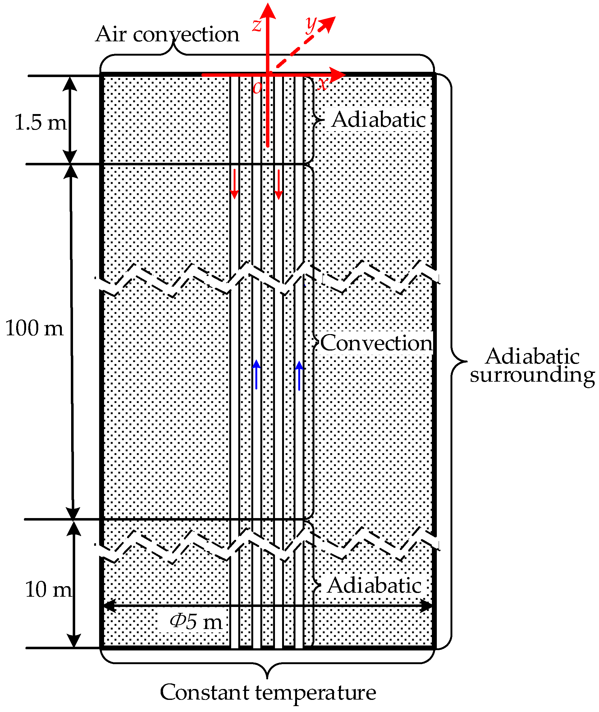
2. Physical and Mathematical Models

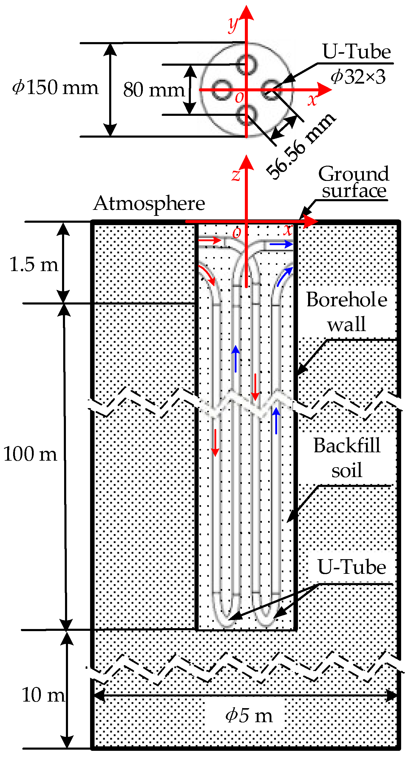
2.1. Physical Model

This paper takes the heat conduction between the double U-tube heat exchanger and the surrounding soil as an example to illustrate the building process of the layered slice algorithm and analyze its solving performance. The corresponding physical model is shown in Figure 1. The heat-storage system mainly includes the double U-tube heat exchanger, backfill soil, and original soil. For low-temperature soil heat storage in practice engineering, the U-tube heat exchanger generally adopts an HDPE pipe with a diameter of 32 mm and a thickness of 3 mm, and the center distance between two adjacent pipes is set as 56.56 mm. The U-tube heat exchanger is buried in a borehole with a diameter of 150 mm and a depth of 101.5 m.

A space of 1.5 m below the ground surface is usually used to arrange horizontal pipes. These horizontal pipes connect the inlets and outlets of double U-tube heat exchangers in multi-boreholes and are covered with a thermal insulation layer on the outside. A space from 1.5 m to 101.5 m is the main body of heat storage. The double U-tube heat exchanger is placed in this space and exchanges heat with the surrounding soil. When the depth and radius are greater than 111.5 m and 2.5 m, respectively, the soil temperature is hardly affected by the ground heat exchanger [39]. Therefore, the computation domain is set to 111.5 m (depth) × 5 m (diameter).

The soil heat storage is affected by many factors. In order to simplify the calculation process, the following reasonable assumptions are put forward, based on the actual situation in the project:

(1)

The backfill still uses the original soil;

(2)

The effective thermophysical properties are adopted instead of the actual soil parameter and are set as constants. Then, the complex coupling process in the soil can be regarded as a single heat conduction problem;

(3)

Water is selected as the working medium in the U-type tube and is assumed to be an incompressible fluid;

(4)

A U-type tube is simplified as two straight tubes with opposite flow directions and equal bottom temperature.

Based on the assumptions above, a simplified physical model for the soil heat-storage system is established in this paper, as shown in Figure 2. It should be noted that we neglect the connection part at the bottom of the U-type tube. Then, the double U-tube heat exchanger is transformed into four straight tubes running from top to bottom. For the four straight tubes, the upper and lower parts are all set as the adiabatic boundary condition. The middle section with a length of 100 m is considered the convection heat-transfer boundary condition. For the simplified physical model, the top, bottom, and outside surfaces are set as the convection heat-transfer, isothermal, and adiabatic boundary conditions, respectively.

2.2. Mathematical Model

2.2.1. Governing Equation for Convection Heat Transfer Inside the Tube

Compared with the tube length, its diameter is so small that it can be neglected. Therefore, it is assumed that the temperature is uniform on the cross-section of the tube. The temperature is only a function of time and the axial position of the tube. Then, the energy equation for the fluid inside the tube can be written as follows:

$$\frac{\partial \left({\rho }_f{c}_f{T}_f\right)}{\partial \tau }+\frac{\partial \left({\rho }_f{c}_f{w}_f{T}_f\right)}{\partial z}=\frac{\partial }{\partial z}\left({\lambda }_f\frac{\partial T_f}{\partial z}\right)+\frac{2h(T_{ts}-T_f)}{r}$$

(1)

where T_f and T_ts refer to the temperatures of the fluid and the inner surface of the tube, h is the coefficient of convection heat transfer, and r is the tube radius. The value of heat transfer coefficient in calculation comes from reference [40].

2.2.2. Governing Equation for Generalized Heat-Storage Body

For convenience, the soil and the tube wall are unified into a generalized heat-storage body. The corresponding energy equation can be expressed as

$$\frac{\partial \left(\rho cT\right)}{\partial \tau }=\frac{\partial }{\partial x}\left(\lambda \frac{\partial T}{\partial x}\right)+\frac{\partial }{\partial y}\left(\lambda \frac{\partial T}{\partial y}\right)+\frac{\partial }{\partial z}\left(\lambda \frac{\partial T}{\partial z}\right)$$

(2)

It should be noted that the subscript is omitted when referring to the generalized heat-storage body. Still, the subscripts t and s are adopted when denoting tube and soil, respectively.

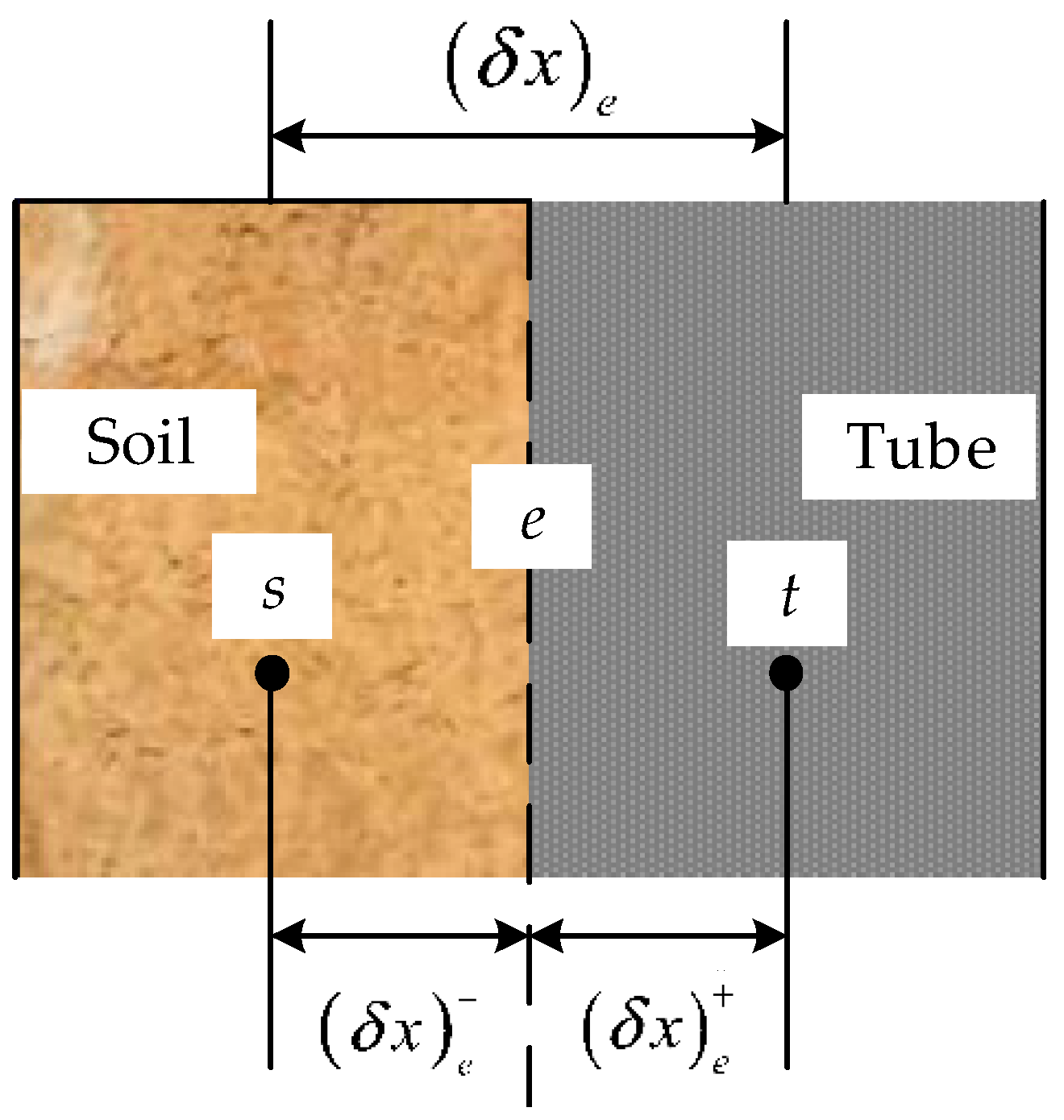
2.2.3. Treatment of Interface between Tube and Soil

As shown in Figure 3, when the thermal contact resistance is ignored, the temperature at the interface e meets

$$T_e|{}_s=T_e|{}_t$$

(3)

The corresponding thermal conductivity coefficient at the interface can be obtained by the harmonic mean method. First, the heat flux through the interface can be calculated by Fourier’s law.

$$q_e=\frac{T_e-T_s}{\frac{{\left(\delta x\right)}_e^{-}}{{\lambda }_s}}=\frac{T_t-T_e}{\frac{{\left(\delta x\right)}_e^{+}}{{\lambda }_t}}=\frac{T_t-T_s}{\frac{{\left(\delta x\right)}_e^{-}}{{\lambda }_s}+\frac{{\left(\delta x\right)}_e^{+}}{{\lambda }_t}}=\frac{T_t-T_s}{\frac{{\left(\delta x\right)}_e}{{\lambda }_e}}$$

(4)

Then, the following Equation can be obtained from the above Equation.

$$\frac{{\left(\delta x\right)}_e^{-}}{{\lambda }_s}+\frac{{\left(\delta x\right)}_e^{+}}{{\lambda }_t}=\frac{{\left(\delta x\right)}_e}{{\lambda }_e}$$

(5)

Finally, we obtain the thermal conductivity coefficient at the interface.

$${\lambda }_e=\frac{{\left(\delta x\right)}_e}{\frac{{\left(\delta x\right)}_e^{-}}{{\lambda }_s}+\frac{{\left(\delta x\right)}_e^{+}}{{\lambda }_t}}$$

(6)

2.2.4. Boundary Conditions

In Section 2.1, the types of boundary conditions have been introduced for the different surfaces in the simplified physical model. In the following, we give the corresponding expressions of these boundary conditions.

For the four straight tubes, the upper, middle, and lower sections’ temperature boundary conditions are expressed as follows:

$${\lambda }_t\frac{\partial T_t}{\partial n_t}=0 \mathrm{at}\{\begin{array}{l}{\left(x+0.04\right)}^2+y^2=0, -1.5 \mathrm{m}\le z\le 0\\ {\left(x-0.04\right)}^2+y^2=0, -1.5 \mathrm{m}\le z\le 0\\ x^2+{\left(y+0.04\right)}^2=0, -1.5 \mathrm{m}\le z\le 0 \\ x^2+{\left(y-0.04\right)}^2=0, -1.5 \mathrm{m}\le z\le 0\end{array}$$

(7)

$${\lambda }_t\frac{\partial T_t}{\partial n_t}=h_f\left(T_t-T_f\right) \mathrm{at}\{\begin{array}{l}{\left(x+0.04\right)}^2+y^2=0, -101.5 \mathrm{m}\le z\le -1.5 \mathrm{m}\\ {\left(x-0.04\right)}^2+y^2=0, -101.5 \mathrm{m}\le z\le -1.5 \mathrm{m}\\ x^2+{\left(y+0.04\right)}^2=0, -101.5 \mathrm{m}\le z\le -1.5 \mathrm{m}\\ x^2+{\left(y-0.04\right)}^2=0, -101.5 \mathrm{m}\le z\le -1.5 \mathrm{m}\end{array}$$

(8)

$${\lambda }_t\frac{\partial T_t}{\partial n_t}=0 \mathrm{at}\{\begin{array}{l}{\left(x+0.04\right)}^2+y^2=0, -111.5 \mathrm{m}\le z\le -101.5 \mathrm{m}\\ {\left(x-0.04\right)}^2+y^2=0, -111.5 \mathrm{m}\le z\le -101.5 \mathrm{m}\\ x^2+{\left(y+0.04\right)}^2=0, -111.5 \mathrm{m}\le z\le -101.5 \mathrm{m}\\ x^2+{\left(y-0.04\right)}^2=0, -111.5 \mathrm{m}\le z\le -101.5 \mathrm{m}\end{array}$$

(9)

where n_t refers to the normal direction pointing toward the tube wall, h_f is the convection heat transfer coefficient for water, and t_f denotes the water temperature.

For the simplified physical model, the temperature boundary conditions of the top, bottom, and outside surfaces are, respectively, described as

$${\lambda }_s\frac{\partial T_s}{\partial n_s}=h_a\left(T_s-T_a\right) \mathrm{at} z=0$$

(10)

$$T_s=T_c \mathrm{at} z=-111.5 \mathrm{m}$$

(11)

$${\lambda }_s\frac{\partial T_s}{\partial n_s}=0 \mathrm{at} {\left(x-2.5\right)}^2+{\left(y-2.5\right)}^2=0$$

(12)

where n_s refers to the normal direction pointing toward the soil, h_a is the convection heat transfer coefficient for air, t_a denotes the air temperature, and T_c is a set temperature.

3. Numerical Simulation Method

3.1. Traditional 3D Simulation Algorithm

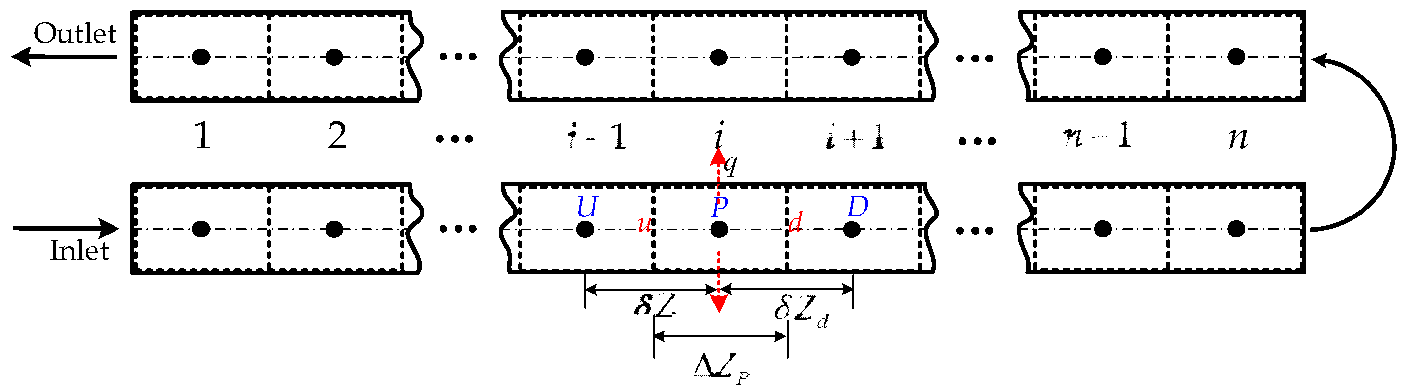
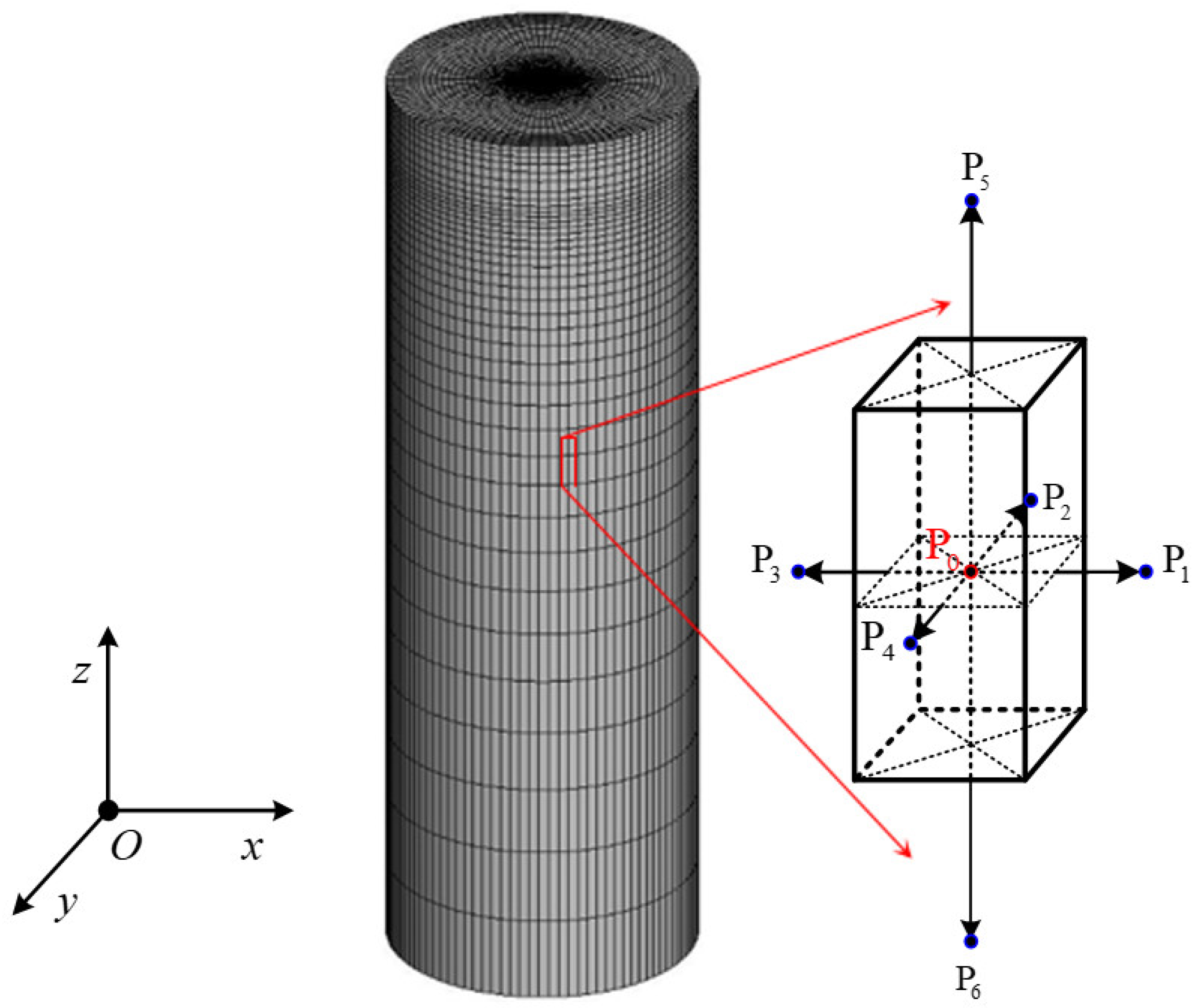
3.1.1. Discretization of the Computation Domain

We adopt a one-dimensional grid system to calculate the temperature change along the tube (see Figure 4). For this grid system, each control volume is a cylinder whose diameter is equal to the tube’s inner diameter.

For the generalized heat-storage body region, the unstructured quadrilateral grid is adopted on the horizontal section, as shown in Figure 5. The temperature changes sharply in and near the tube wall, so the mesh is refined locally in this area. Along the depth direction, the structures of different horizontal sections are the same as each other. Therefore, a structured grid is made in the depth direction. Then, the corresponding 3D grid system is generated, and each control volume is a quadrangular prism (see Figure 6).

3.1.2. Discretization and Solution of Energy Equation for In-Tube Fluid

Based on the one-dimensional grid system (see Figure 4), the finite volume method is adopted to discretize the energy Equation (1). Because the in-tube fluid temperature changes little, the corresponding thermophysical properties such as density, specific heat capacity, and thermal conductivity are assumed to be constant.

If we integrate Equation (1) over the control volume around the central grid point P, we obtain:

$${\displaystyle {\int }_u^d\frac{\partial \left({\rho }_f{c}_f{T}_f\right)}{\partial \tau }}{A}_{t}dz+{\displaystyle {\int }_u^d\frac{\partial \left({\rho }_f{c}_f{w}_f{T}_f\right)}{\partial z}}{A}_{t}dz={\displaystyle {\int }_u^d\frac{\partial }{\partial z}\left({\lambda }_f\frac{\partial T_f}{\partial z}\right)A_{t}dz}+{\displaystyle {\int }_u^d\frac{2h(T_{ts}-T_f)}{r}{A}_{t}dz}$$

(13)

where u and d refer to the upstream and downstream faces of the control volume, A_t is the tube’s cross-sectional area.

When we adopt an explicit time-integration scheme combined with a first-order upwind spatial scheme, the following discretization equation can be obtained:

$${\rho }_f{c}_f\frac{\left(T_{f,P}-T_{f,P}^0\right)}{\Delta \tau }\Delta V+\left[\begin{array}{l}{\rho }_f{c}_f{w}_f{T}_{f,P}^0{A}_t\\ -{\rho }_f{c}_f{w}_f{T}_{f,U}^0{A}_t\end{array}\right]=\left[{\lambda }_f\left(\frac{T_{f,U}^0-T_{f,P}^0}{\delta z_u}\right)A_t-{\lambda }_f\left(\frac{T_{f,P}^0-T_{f,D}^0}{\delta z_d}\right)A_t\right]+2\pi r\Delta z_{P}h\left(T_{ts,P}^0-T_{f,P}^0\right)$$

(14)

where the superscript 0 refers to the current time step, the subscripts U and D denote the upstream and downstream grid points, $\Delta V$ is the volume of the control volume, and $\Delta \tau$ is the time step. According to the known temperatures at the current time step, we can obtain the fluid temperature at the next time step by solving Equation (14). Then, the calculated fluid temperature can be used as the boundary condition to compute the generalized heat-storage body’s temperature field.

3.1.3. Discretization and Solution of Energy Equation for Generalized Heat-Storage Body

Figure 6 shows the 3D grid system for the generalized heat-storage body. We focus attention on the central grid point P₀, which has the grid points P₁, P₂, P₃, P₄, P₅, P₆ as its neighbors. If we integrate Equation (2) over the control volume around P₀, we obtain:

$${\displaystyle \underset{V}{\int }\frac{\partial \left(\rho cT\right)}{\partial \tau }}dV={\displaystyle \underset{V}{\int }\nabla }\cdot \left(\lambda \nabla T\right)dV$$

(15)

The unsteady term in Equation (15) can be expanded to obtain:

$${\displaystyle \underset{V}{\int }\frac{\partial \left(\rho cT\right)}{\partial \tau }}dV=\rho c_p{V}_{P_0}\frac{T_{P_0}-T_{P_0}^0}{\Delta \tau }$$

(16)

where $V_{P_0}$ denotes the volume of the control volume.

For the diffusion term in Equation (15), we obtain:

$${\displaystyle \underset{V}{\int }\nabla }\cdot \left(\lambda \nabla T\right)dV=\lambda {\displaystyle \underset{A}{\int }\left(\nabla T\right)\cdot d\mathit{A}}={\displaystyle \sum _{j=1}^6\lambda {\left(\nabla T\right)}_j\cdot }{\mathit{A}}_j={\displaystyle \sum _{j=1}^6\left(D_j^n+D_j^c\right)}$$

(17)

where $D_j^n$ and $D_j^c$ refer to the normal and cross diffusion fluxes, respectively. The corresponding expressions are:

$$D_j^n=\lambda \left(\frac{T_{P_j}-T_{P_0}}{\left|{\mathit{d}}_j\right|}\frac{{\mathit{d}}_j}{\left|{\mathit{d}}_j\right|}\right)\cdot {\mathit{A}}_j$$

(18)

$$D_j^c=\lambda \left[{\left(\nabla T\right)}_j^0-{\left(\nabla T\right)}_j^0\cdot \frac{{\mathit{d}}_j}{\left|{\mathit{d}}_j\right|}\frac{{\mathit{d}}_j}{\left|{\mathit{d}}_j\right|}\right]\cdot {\mathit{A}}_j$$

(19)

Substituting Equations (18) and (19) into Equation (17), we obtain:

$${\displaystyle \underset{V}{\int }\nabla }\cdot \left(\lambda \nabla T\right)dV={\displaystyle \sum _{j=1}^6\left\{\lambda \left(\frac{T_{P_j}-T_{P_0}}{\left|{\mathit{d}}_j\right|}\frac{{\mathit{d}}_j}{\left|{\mathit{d}}_j\right|}\right)\cdot {\mathit{A}}_j+\lambda \left[{\left(\nabla T\right)}_j^0-{\left(\nabla T\right)}_j^0\cdot \frac{{\mathit{d}}_j}{\left|{\mathit{d}}_j\right|}\frac{{\mathit{d}}_j}{\left|{\mathit{d}}_j\right|}\right]\cdot {\mathit{A}}_j\right\}}$$

(20)

where ${\mathit{A}}_j$ denotes the area vector of the control-volume face j, ${\left(\nabla T\right)}_j^0$ is the temperature gradient at the control-volume face j. The value of ${\left(\nabla T\right)}_j^0$ can be obtained by the following linear interpolation:

$${\left(\nabla T\right)}_j^0=w_{p_0}{\left(\nabla T\right)}_{p_0}^0+w_{p_j}{\left(\nabla T\right)}_{p_j}^0$$

(21)

where $w_{p_0}$ and $w_{p_j}$ are interpolation factors. ${\left(\nabla T\right)}_{p_0}^0$ and ${\left(\nabla T\right)}_{p_j}^0$ are the temperature gradients at the grid points P₀ and P_j, which can be calculated by the least square method [41].

Substituting Equations (16) and (20) into Equation (15), we obtain the corresponding discretization equation:

$$a_{p_0}{T}_{p_0}={\displaystyle \sum _{j=1}^6{a}_{p_j}{T}_{p_j}}+b_{P_0}$$

(22)

where

$$a_{p_j}=\lambda \frac{{\mathit{d}}_j\cdot {\mathit{A}}_j}{{\left|{\mathit{d}}_j\right|}^2}\hspace{1em}j=1~6$$

(23)

$$a_{p_0}=\rho c\frac{V_{p_0}}{\Delta \tau }+{\displaystyle \sum _{j=1}^6{a}_{p_j}}$$

(24)

$$b_{P_0}=\rho c\frac{V_{p_0}}{\Delta \tau }{T}_{P_0}^0+{\displaystyle \sum _{j=1}^6\lambda \left[\left(w_{p_0}{\left(\nabla T\right)}_{p_0}^0+w_{p_j}{\left(\nabla T\right)}_{p_j}^0\right)-\left(w_{p_0}{\left(\nabla T\right)}_{p_0}^0+w_{p_j}{\left(\nabla T\right)}_{p_j}^0\right)\cdot \frac{{\mathit{d}}_j}{\left|{\mathit{d}}_j\right|}\frac{{\mathit{d}}_j}{\left|{\mathit{d}}_j\right|}\right]\cdot {\mathit{A}}_j}$$

(25)

According to the known temperature, time step, mesh geometry parameters, and thermophysical properties, we can calculate the coefficients $a_{p_0}$, $a_{p_j}$ and source term $b_{P_0}$ in Equation (22). Then, the discretization equations for all grid points are iteratively solved in the whole 3D space. Finally, we can obtain the unknown temperature field at the next time step.

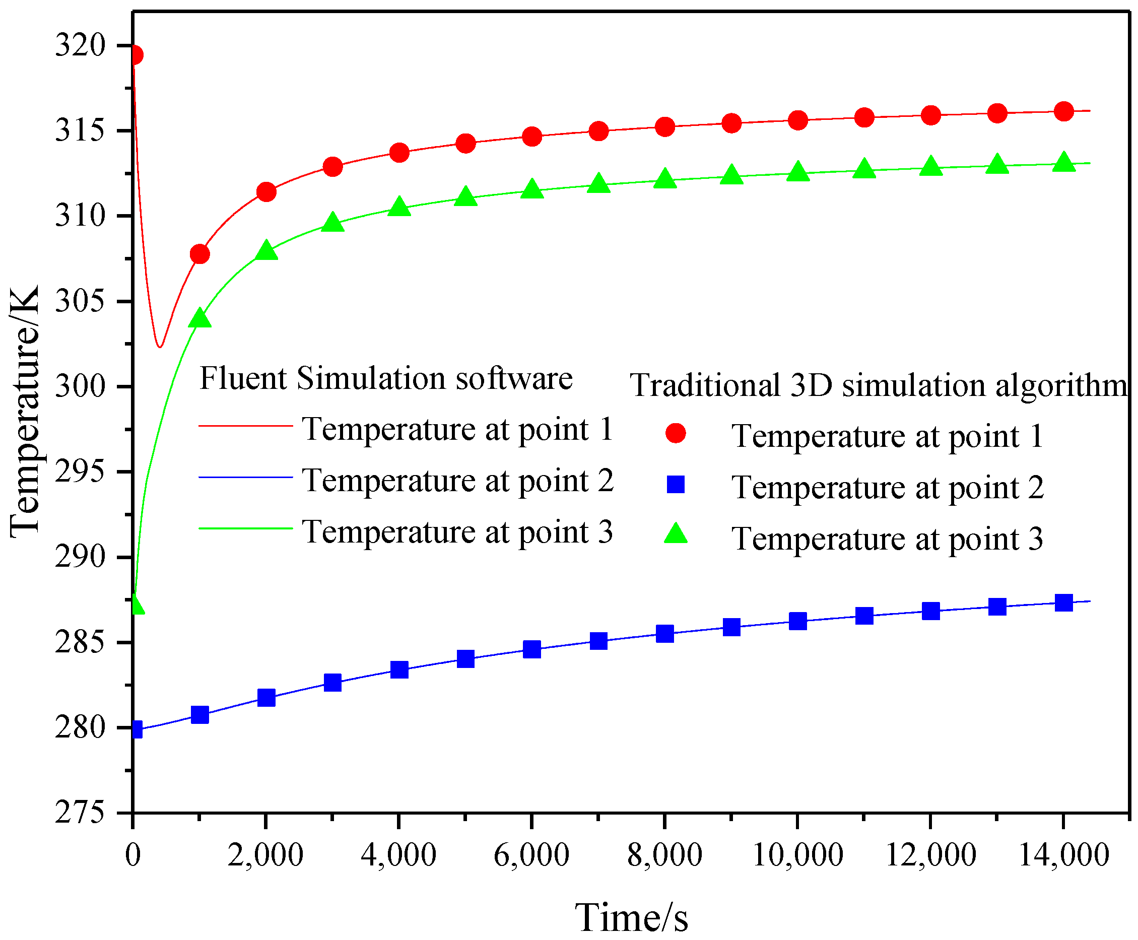
3.1.4. Traditional 3D Simulation Algorithm Self-Programming Accuracy Verification

In order to verify the correctness of the traditional 3D simulation algorithm, this chapter developed the solution program of the traditional 3D simulation algorithm according to the above discrete equations and solving steps. Then, the solution program of the traditional 3D simulation algorithm and FLUENT software were, respectively, used to simulate the soil heat storage process for 4 h. Finally, the simulation results of traditional 3D simulation algorithm are compared and verified.

In the following example, the same mesh quantity (600,000) and the same time step (10 s) are used. The physical parameters of raw soil, backfill soil, pipe wall and heat carrying medium are set, as shown in

Table 1. Thermophysical properties of soil, tube wall, and in-tube fluid.

Medium	Thermal Conductivity Coefficient λ [W/(m·K)]	Density ρ [kg/m3]	Specific Heat cp [J/(kg·K)]
Soil	1.40	1500.0	848.0
Tube wall	0.35	1230.0	1510.0
In-tube fluid	0.64	988.1	4181.5

.

In this example, the temperature field of soil heat storage was simulated under the condition that the inlet temperature was constant at 323 K, and the temperature changes with time at points 1 (0.04, 0, 0) (exit of U-shaped pipe), 2 (−0.06, 0.01, −1.5) and 3 (−0.03, 0.03, −101.5) were recorded, as shown in Figure 7. As can be seen from the figure, the results obtained by the solution program of the traditional 3D simulation algorithm in the whole heat storage process are almost identical with those obtained by the FLUENT software.

In order to quantitatively analyze the accuracy of the traditional 3D simulation algorithm,

Table 2. Temperature errors at observation points calculated by the traditional 3D simulation algorithm under thermal storage condition.

Error	Point 1	Point 2	Point 3
Absolute error [K]	0.0095	0.019	0.039
Relative error [%]	0.056	0.25	0.15

lists the maximum temperature errors at the three points in the whole heat storage process. As listed in the table, compared with the results calculated by the Fluent software, the absolute temperature errors for the traditional 3D simulation algorithm are all less than 0.039 K, and the relative errors are all less than 0.25%.

Next, we will propose a layered slice algorithm based on the traditional 3D algorithm and analyze its performance in depth.

3.2. Layered Slice Algorithm

The above traditional 3D simulation algorithm needs to simultaneously solve the discrete equations in the whole 3D space, making convergence difficult and time-consuming. According to the structural and heat transfer characteristics of the simplified physical model, this paper proposes a layered slice algorithm, which transforms the 3D solution process into the solutions of 2D heat transfer on different horizontal slices.

The in-tube calculation process is the same for the traditional 3D simulation algorithm and the layered slice algorithm. The essential difference between these two algorithms lies in the energy equation’s discretization and solution for the generalized heat-storage body.

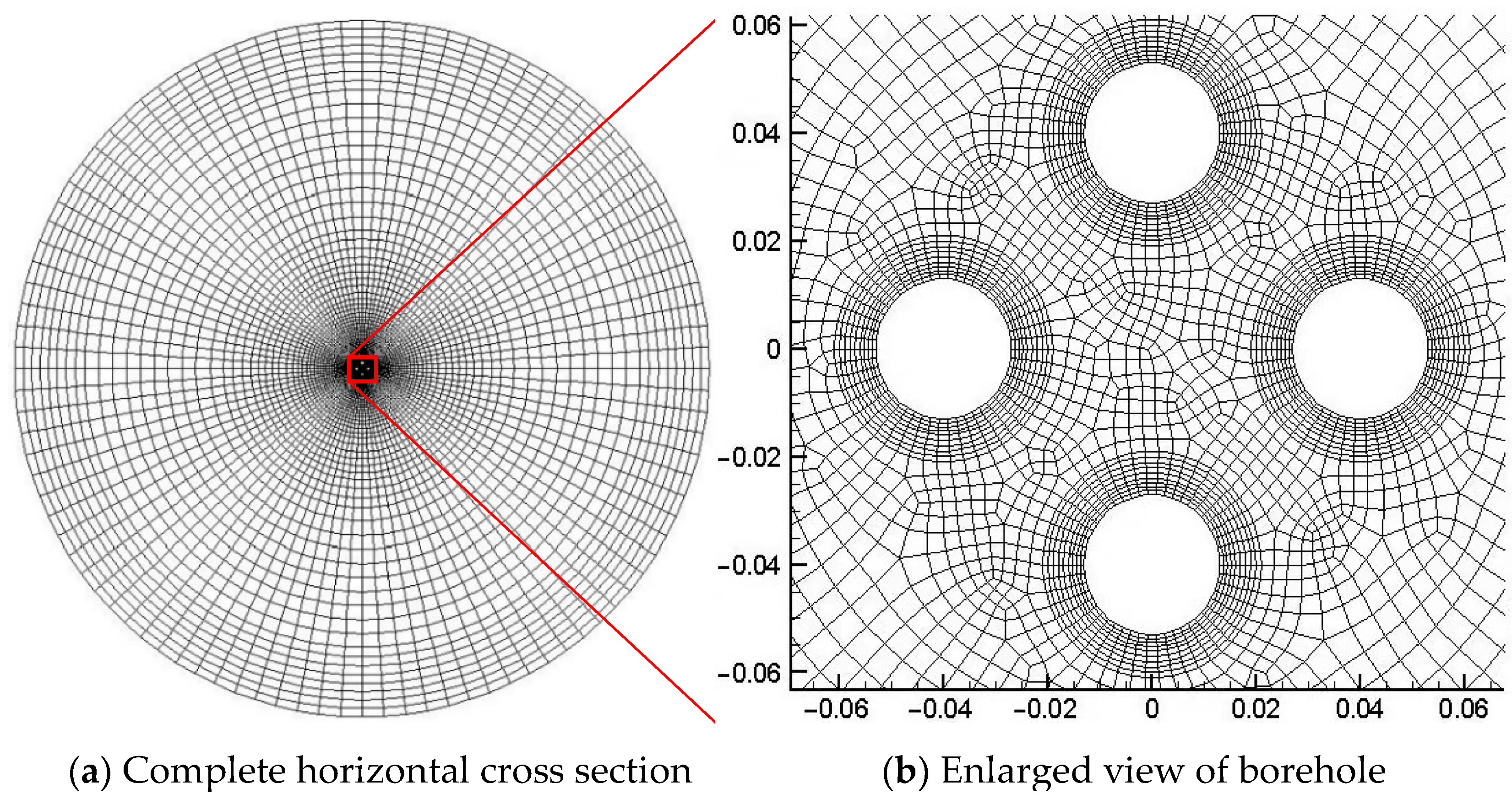
3.2.1. Discretization of the Computation Domain

The discrete Equation (22) used in the traditional 3D simulation algorithm is split into the horizontal and vertical directions and is written as:

$$\left(\rho c\frac{V_{p_0}}{\Delta \tau }+{\displaystyle \sum _{j=1}^4{a}_{p_j}+{\displaystyle \sum _{j=5}^6{a}_{p_j}}}\right)T_{p_0}={\displaystyle \sum _{j=1}^4{a}_{p_j}{T}_{p_j}}+{\displaystyle \sum _{j=5}^6{a}_{p_j}}{T}_{p_j}+b_{P_0}$$

(26)

Considering the characteristic of a high heat-transfer rate in the horizontal direction while low in the vertical direction, we adopt the known temperatures to calculate the heat transfer in the vertical direction. Thus, the above equation can be cast into the following form:

$$\left(\rho c\frac{V_{p_0}}{\Delta \tau }+{\displaystyle \sum _{j=1}^4{a}_{p_j}}\right)T_{p_0}={\displaystyle \sum _{j=1}^4\left(a_{p_j}{T}_{p_j}\right)}+{\displaystyle \sum _{j=5}^6\left[a_{p_j}\left(T_{p_j}^0-T_{p_0}^0\right)\right]}+b_{P_0}$$

(27)

The latter two terms on the right side of Equation (27) can be unified into a new source term:

$$B_{P_0}={\displaystyle \sum _{j=5}^6\left[a_{p_j}\left(T_{p_j}^0-T_{p_0}^0\right)\right]}+b_{P_0}$$

(28)

Finally, we can obtain the discrete energy equation involved in the layered slice algorithm. The result is:

$$a_{p_0}{T}_{p_0}={\displaystyle \sum _{j=1}^4{a}_{p_j}{T}_{p_j}}+B_{P_0}$$

(29)

where

$$a_{p_j}=\lambda \frac{{\mathit{d}}_j\cdot {\mathit{A}}_j}{{\left|{\mathit{d}}_j\right|}^2}\hspace{1em}j=1~4$$

(30)

$$a_{p_0}=\rho c\frac{V_{p_0}}{\Delta \tau }+{\displaystyle \sum _{j=1}^4{a}_{p_j}}$$

(31)

There are just horizontal-direction unknown temperatures in Equation (29), so the 3D solution process is successfully transformed into 2D heat transfer solutions on different horizontal slices.

3.2.2. Solution Procedure of Layered Slice Algorithm

To better understand the layered slice algorithm, we will introduce its detailed solution procedure in the following:

Step 1: Build the simplified physical model for the soil heat-storage system (see Figure 2), which has the same structures for different horizontal slices;

Step 2: Establish the energy Equations (1) and (2) for the in-tube fluid and the generalized heat-storage body, respectively;

Step 3: Set the thermophysical properties, the boundary conditions, and the initial temperatures;

Step 4: Generate the 1D and 3D grid systems (see Figure 4 and Figure 6) for the in-tube fluid and the generalized heat-storage body, respectively. The 3D grid system adopts the same 2D unstructured grids on different horizontal slices for implementing the layered slice algorithm;

Step 5: Derive the discrete energy Equations (14) and (29) for the in-tube fluid and the generalized heat-storage body, respectively.

Step 6: Solve the discrete energy Equation (14) according to the known temperatures at the current time step and then obtain the next time step’s fluid temperature. Note that the calculated fluid temperature can be used to update the boundary condition for the generalized heat-storage body;

Step 7: Calculate the coefficients and source term in the discrete energy Equation (29) according to the known temperatures. Then, solve the equation slice by slice to obtain the temperature distribution within the generalized heat-storage body at the next time step; Note that the solving processes for different horizontal slices are entirely independent. We can calculate one slice and then another.

Step 8: Regard the calculated temperature as the known, then return to Step 6 for the next time step.

Repeat Steps 6~8 until the time reaches the preset value.

4. Numerical Comparisons and Analyses

The temperature distribution during soil heat storage may be affected by the thermophysical properties of soil, tube wall, and in-tube fluid. However, they have little influence on the solving performance of the proposed layered slice algorithm. Therefore, we adopt the specific thermophysical properties (see Table 1) to study and analyze the proposed algorithm through some different cases. It should be noted that the programming language used for both algorithms is Fortran90, and the computer used in the test has eight computing cores and 16 threads. In Section 4.1 and Section 4.2, only single-thread serial computation is used in the test example, while in Section 4.3, 1~16 threads are used for parallel computation with OpenMP fortran application program interface.

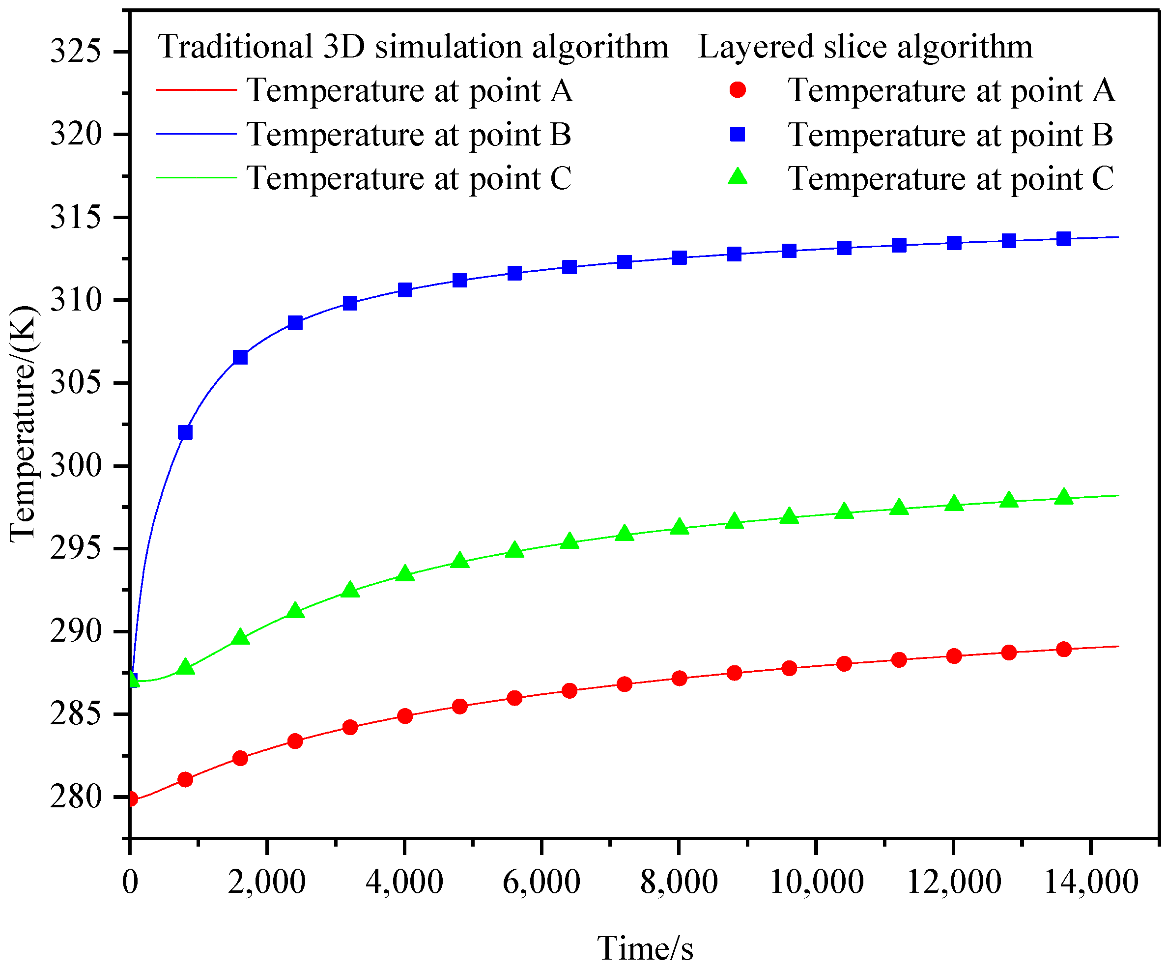
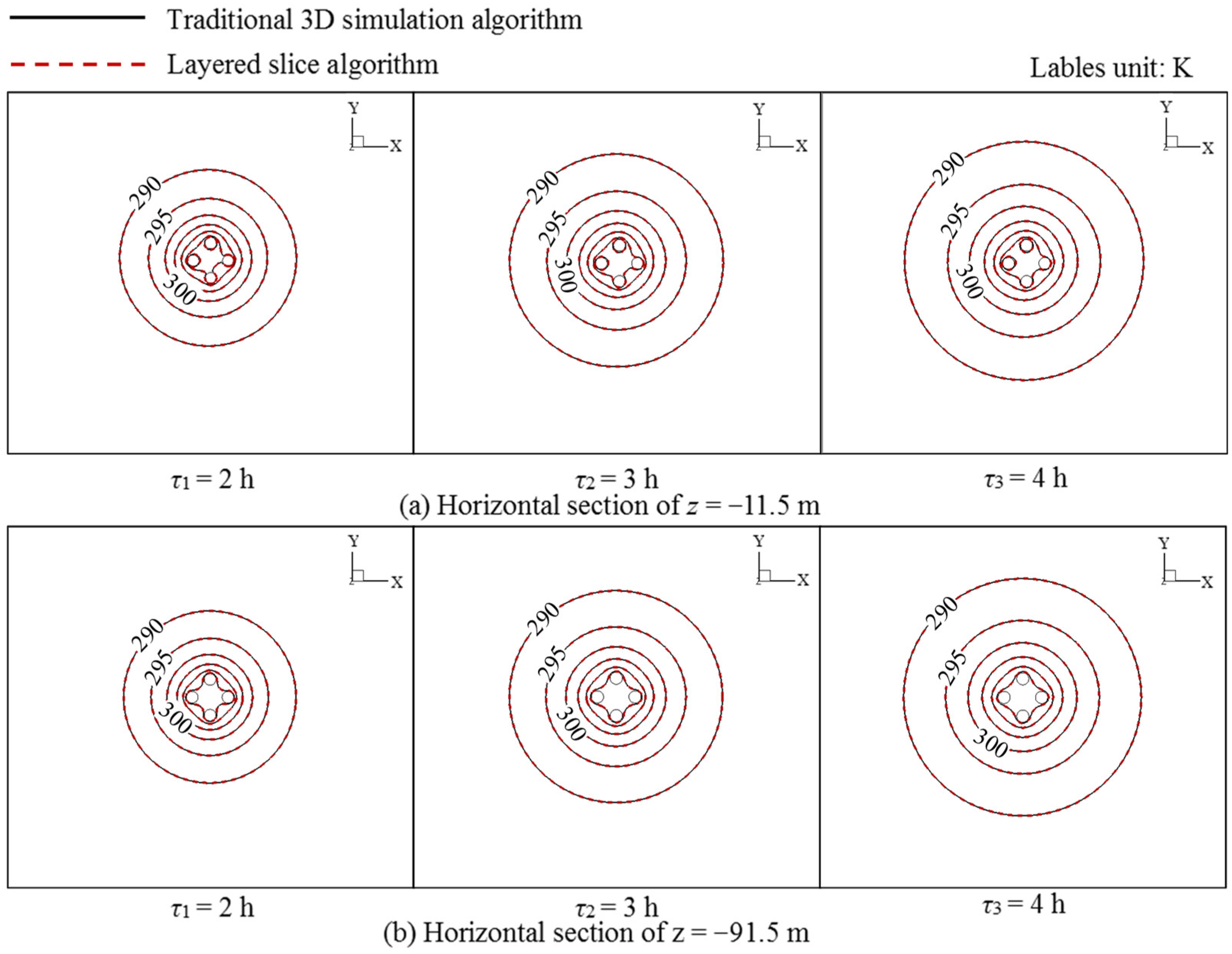
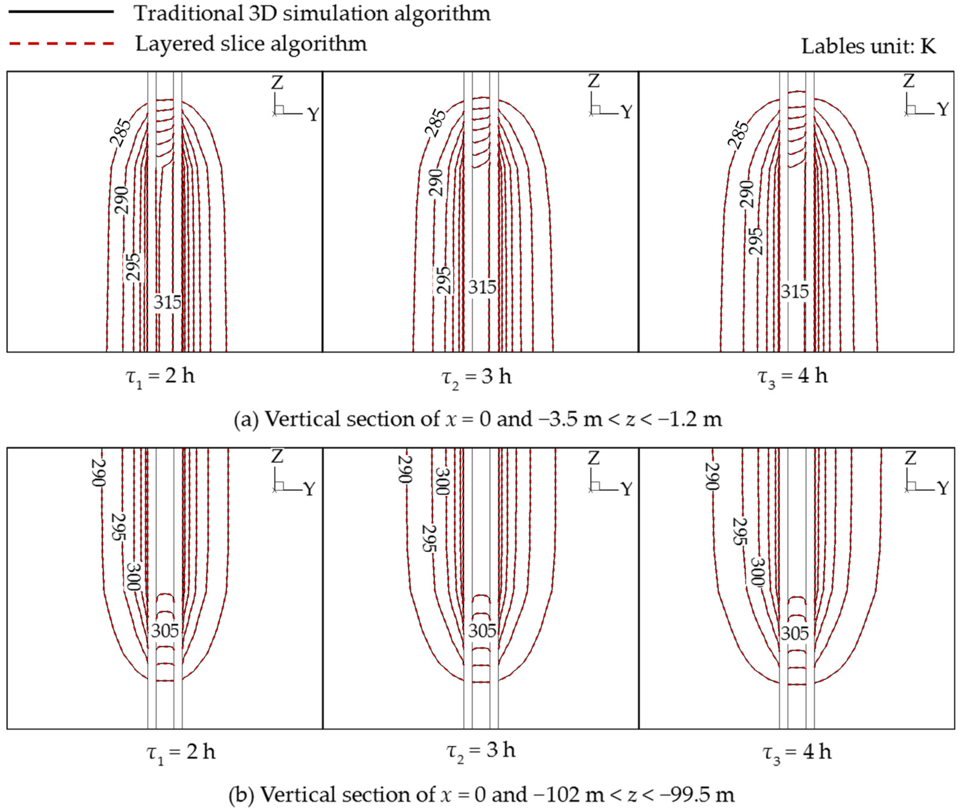
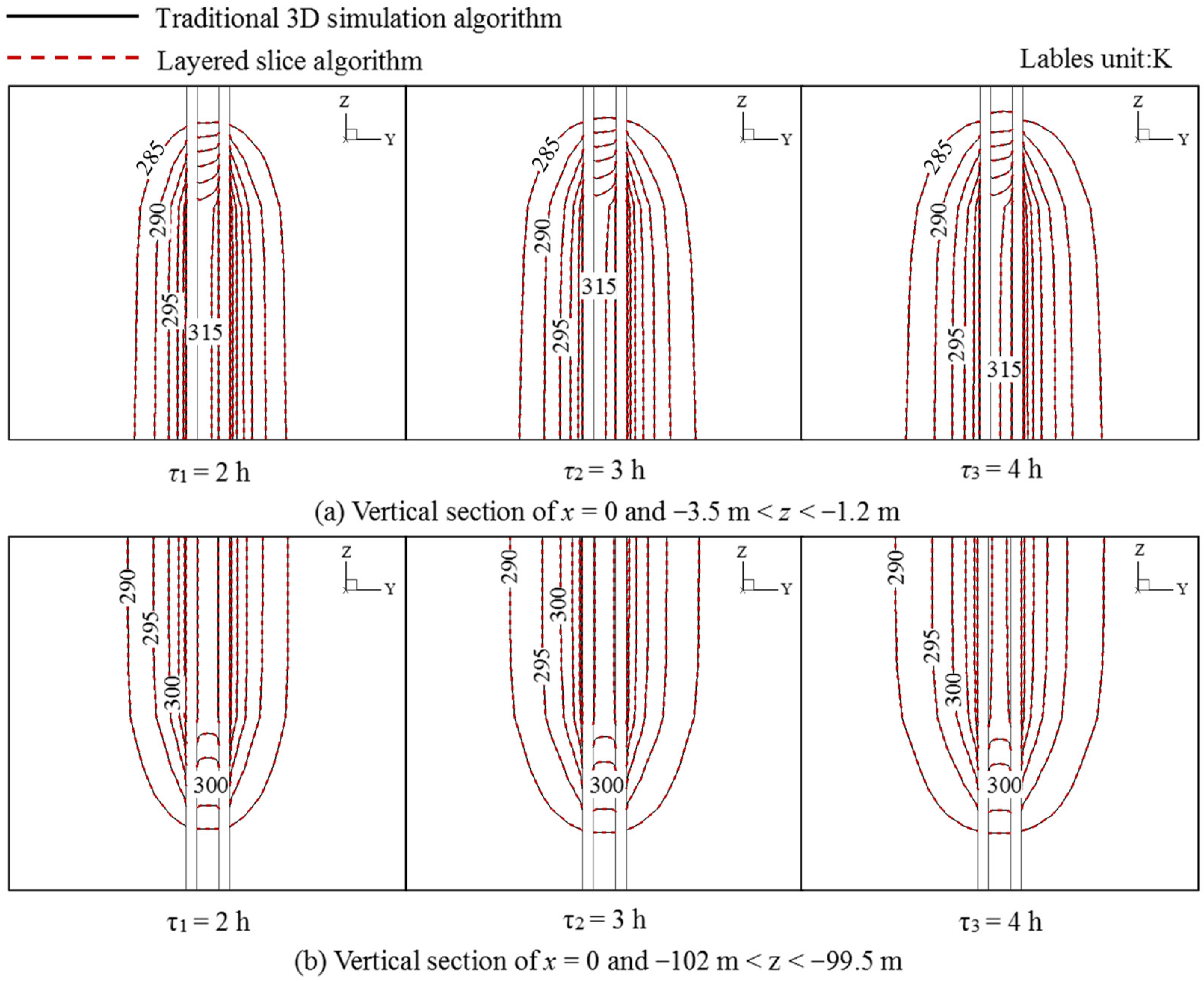
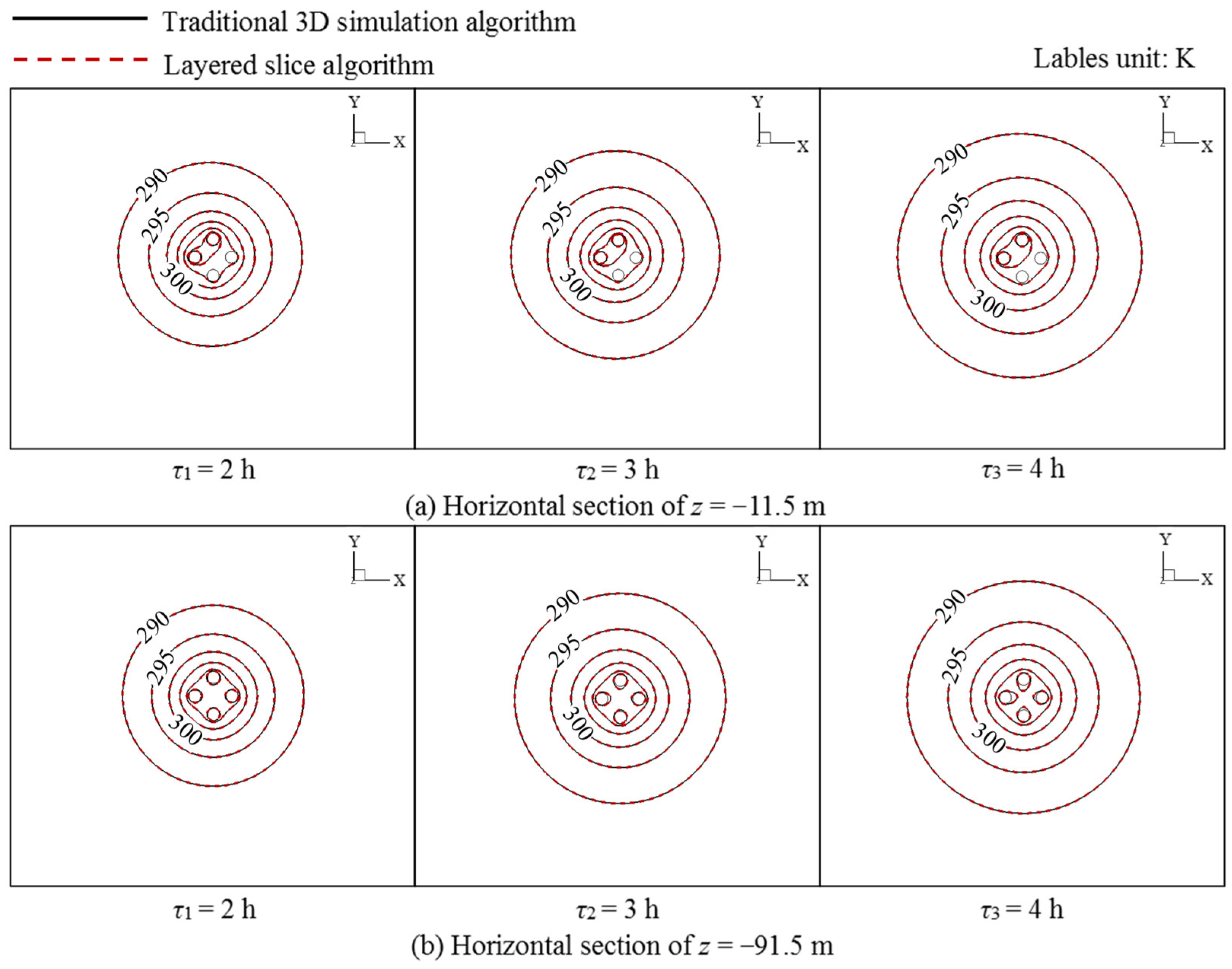
4.1. Accuracy Verification of Layered Slice Algorithm

The inlet temperatures of the double U-tube heat exchanger are mainly divided into two types: fixed and periodic. Based on these two types of temperature conditions, we verify the accuracy of the proposed layered slice algorithm by comparing with the traditional 3D simulation algorithm.

4.1.1. Fixed Inlet Temperature

Table 3. The parameters used in the initial and boundary conditions.

Parameter	Value
Initial temperature of the soil	$T(z)=12.9e^{-0.3\left|z\right|}\cos (0.3|z|-4.13)+287$
Initial temperature of the in-tube fluid	323 K
Fixed inlet temperature	323 K
Periodic inlet temperature	$T_{in}=323.0+5.0\sin \left(\frac{2\pi }{3600}\tau \right)$
Inlet velocity	0.5 m/s
Air temperature	303 K

lists the related parameters used in the initial and boundary conditions. As we know, the soil temperature is affected by the depth and tends to be stable after reaching a certain depth. According to the reference [40], its initial temperature is given as a function of soil depth.

$$T(z)=12.9e^{-0.3\left|z\right|}\cos (0.3|z|-4.13)+287$$

(32)

Besides, the double U-tube heat exchanger’s inlet temperature and velocity are set to 323 K and 0.5 m/s, respectively. The simulation is implemented under the conditions of the grid number with 600,000, the time step with 10 s, and the heat storage time with 4 h. It should be noted that the grid-independent result can be obtained when the grid number is greater than or equal to 600,000.

Because the soil has a large thermal inertness, the temperature change in the area away from the heat exchanger is relatively slow. For better validating the proposed layered slice method, three different points near the U-tube are selected for analysis. These three points are located at different depths and different horizontal positions, which are points A (0, 0, −1.5), B (0.03, 0.03, −54.0) and C (0.075, 0.075, −101.5). Figure 8 illustrates the temperature change at these three points for the case of fixed inlet temperature.

As shown in this figure, the temperature-time change curves calculated by the proposed algorithm are almost completely consistent with the results of the traditional 3D simulation algorithm. In order to quantitatively analyze the accuracy of the proposed algorithm,

Table 4. Temperature errors of the layered slice algorithm at points A, B, and Cunder the condition of fixed inlet temperature.

Error	Point A	Point B	Point C
Absolute error [K]	0.017	3.0 × 10−6	0.0019
Relative error [%]	0.18	0.000011	0.017

lists the maximum temperature errors at the three points in the whole heat storage process. As listed in the table, the temperature errors are very small at point B near the middle of the U-tube, while the errors increase a little at points A and C near either end of the U-tube. The reason is that the heat transfer in the vertical direction at points A and C is larger than that at point B. When we adopt the known temperatures to calculate the heat transfer in the vertical direction, points A and C will produce a larger error. In general, compared with the traditional 3D simulation algorithm, the absolute temperature errors for the proposed layered slice algorithm are all less than 0.017 K, and the relative errors are all less than 0.18%.

In order to further analyze the accuracy of the proposed layered slice algorithm, we compare the instantaneous temperature fields computed by the two different algorithms, as shown in Figure 9 and Figure 10. Their calculation results agree very well with each other in both vertical and horizontal sections, further proving that the layered slice algorithm has a high precision for the case of fixed inlet temperature.

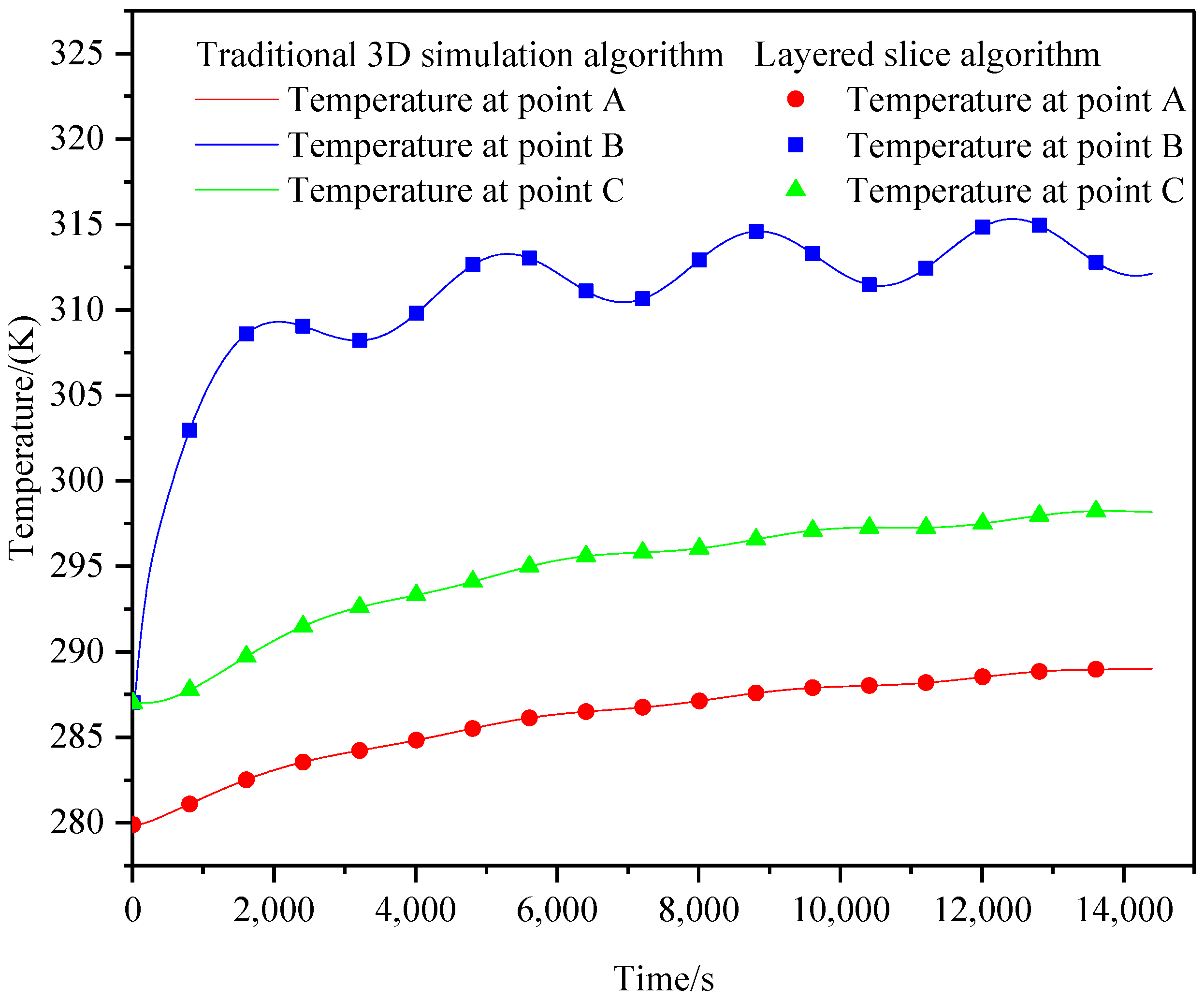
4.1.2. Periodic Inlet Temperature

When the inlet temperature changes periodically, the soil temperature field will fluctuate accordingly. In order to verify the accuracy of the proposed layered slice algorithm for the case of periodic inlet temperature, the inlet temperature is set as a sine function of time.

$$T_{in}=323.0+5.0\sin \left(\frac{2\pi }{3600}\tau \right)$$

(33)

Besides, other conditions are the same as the case of fixed inlet temperature.

In this case, we also compare the temperature changes with time at points A, B, and C, as shown in Figure 11. The three points’ temperatures show an upward trend in fluctuation, and the temperature change curves calculated by the two different algorithms are almost identical.

Table 5. Temperature errors of the layered slice algorithm at points A, B, and Cunder the condition of periodic inlet temperature.

Error	Point A	Point B	Point C
Absolute error [K]	0.017	8.8 × 10−4	0.0021
Relative error [%]	0.19	0.0031	0.019

lists the corresponding temperature errors of the layered slice algorithm. For points A and C, the temperature errors are basically the same as those under the fixed inlet temperature. For point B, the errors are still very small, but they have a little increase compared with the fixed inlet temperature. The reason is that the temperature fluctuations will cause the rise of the heat transfer in the vertical direction, leading to an increase in the layered slice algorithm’s calculation errors. On the whole, compared with the traditional 3D simulation algorithm, the absolute temperature errors for the proposed layered slice algorithm are all less than 0.017 K, and the relative errors are all less than 0.19%.

We have also compared the instantaneous temperature fields calculated by the two different algorithms, as shown in Figure 12 and Figure 13. Their calculation results are in good agreement in both horizontal and vertical directions, which indicates that the proposed layered slice algorithm has a high accuracy for the case of periodic inlet temperature.

With the arguments above, we can conclude that the proposed layered slice algorithm can maintain a high numerical accuracy. In the following, we will analyze the solution speed of the proposed layered slice algorithm in detail.

4.2. Solution Speed Analysis of Layered Slice Algorithm

Unlike the traditional 3D simulation algorithm, the layered slice algorithm transforms the 3D solution process into 2D heat transfer solutions on different horizontal slices. Due to the reduction of dimensionality, the proposed algorithm has an evident accelerating effect. In the following, based on the case of periodic inlet temperature, we will investigate the influences of grid number and time step on the proposed algorithm’s solution speed, respectively.

4.2.1. The Influence of Grid Number

In order to analyze the effect of the grid number on the solution speed of the proposed layered slice algorithm, three different grid numbers of 600,000, 900,000, and 1,200,000 are considered to simulate the case of periodic inlet temperature.

Table 6. Comparison of solving speed between the layered slice algorithm and the traditional 3D simulation algorithm for three different grid numbers.

Algorithm	Grid Number	Computation Time/s	Speedup Ratio
Traditional 3D simulation algorithm	600,000	1180	—
	900,000	1813	—
	1,200,000	2494	—
Layered slice algorithm	600,000	505	2.34
	900,000	768	2.36
	1,200,000	1048	2.38

lists the speedup ratios of the proposed layered slice algorithm over the traditional 3D simulation algorithm and the corresponding computation times. For the grid numbers of 600,000, 900,000, and 1,200,000, the speedup ratios are 2.34, 2.36, and 2.38, respectively. The proposed algorithm has good acceleration effects under different grid systems. At the same time, the acceleration effect is slightly improved with the increase in the grid number. In other words, compared with the traditional 3D simulation algorithm, the layered slice algorithm can obtain fast-converging solutions on different grids.

4.2.2. The Influence of Time Step

Three different time steps of 1 s, 10 s, and 100 s are adopted to research the influence of time step on the solution speed of the proposed layered slice algorithm.

Table 7. Comparison of solving speed between the layered slice algorithm and the traditional 3D simulation algorithm for three different time steps.

Algorithm	Time Step/s	Computation Time/s	Speedup Ratio
Traditional 3D simulation algorithm	1	6128	—
	10	1180	—
	100	261	—
Layered slice algorithm	1	2788	2.20
	10	505	2.34
	100	102	2.56

shows the computation times of these two different algorithms and the speedup ratios of the proposed layered slice algorithm over the traditional 3D simulation algorithm.

For the time steps of 1 s, 10 s, and 100 s, the proposed algorithm’s speedup ratios are 2.20, 2.34, and 2.56, respectively. On the one hand, these data show that the proposed algorithm can obtain fast convergent solutions at different time steps; on the other hand, its acceleration effect is improved continuously with the increase in time step. It is noteworthy that the computation time decreases with the rise of the time step. So, a larger time step should be selected as far as possible on the premise of ensuring the calculation accuracy, which can achieve our proposed algorithm’s best performance.

Based on the above analysis, it can be concluded that compared with the traditional algorithm, the proposed layered slice algorithm can improve the calculation speed by 2.2~2.56 times under different grid numbers and time steps. In addition to the above advantages, the proposed algorithm also has an excellent parallel performance. In the following, we will analyze its parallel performance in detail.

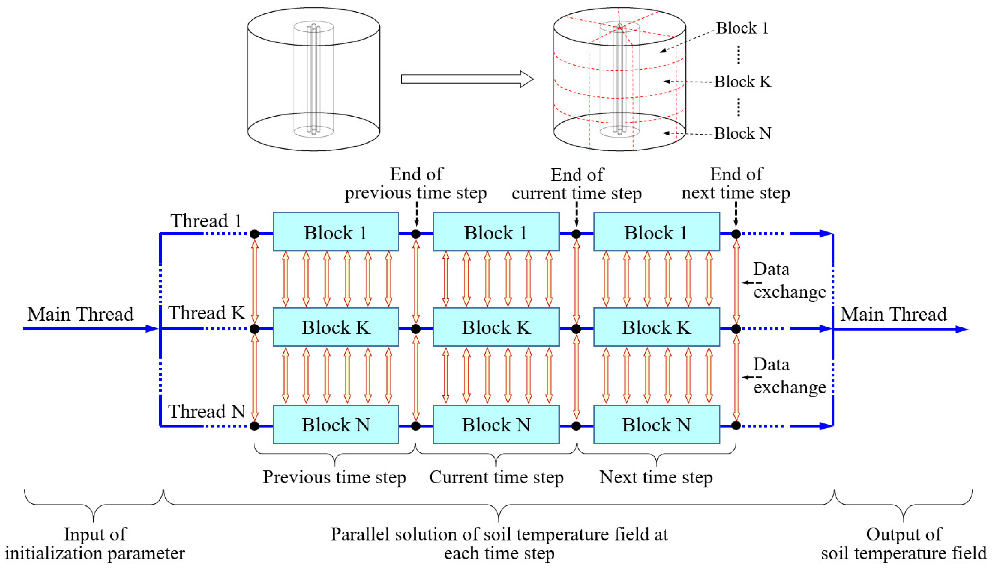
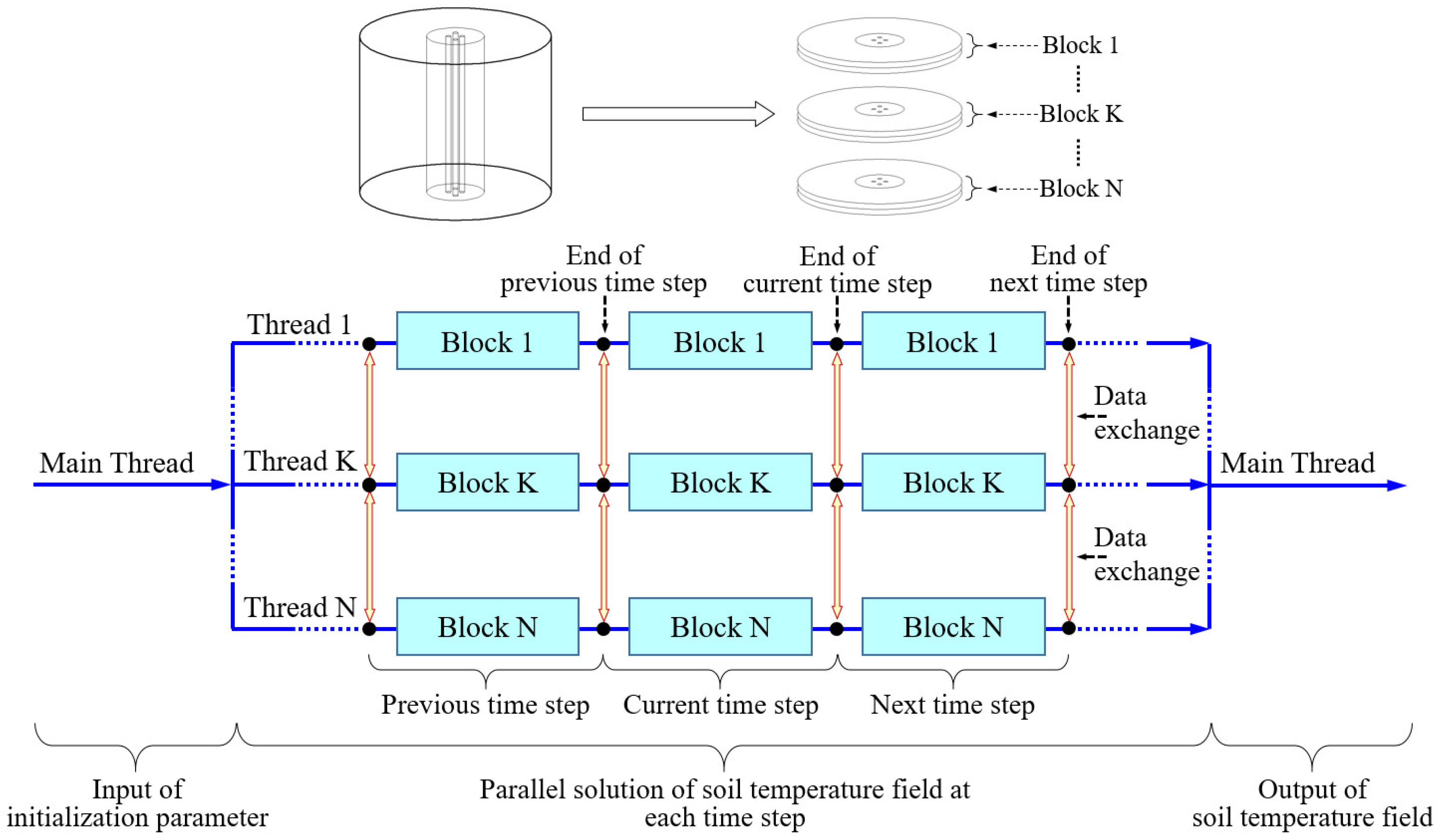
4.3. Parallel Characteristic Analysis of Layered Slice Algorithm

4.3.1. Parallel Computing Principle

In general, parallel computing can be used to speed up the solution of soil heat storage. Figure 14 shows the parallel computing process of the traditional 3D simulation algorithm. In this process, the data exchanges between different threads are required during the iteration solution at each time step. With the increase in the parallel threads, the amount of data communication is raised substantially, leading to the reduction of parallel computing efficiency.

Unlike the traditional 3D simulation algorithm, the layered slice algorithm adopts the known temperatures to calculate the heat transfer in the vertical direction. Thus, the original 3D solution process is transformed into 2D heat transfer solutions on different horizontal slices. Based on this solving characteristic, several horizontal slices can be defined as a block and assigned to a thread for parallel computing, as shown in Figure 15. In this way, there is no need for data exchange between different threads, except at the end of each time step. Due to the substantial reduction of the data exchange among different threads, the parallel computing efficiency of the layered slice algorithm can be significantly improved. In this paper, OpenMP is introduced into the proposed layered slicing algorithm to realize parallel computing. OpenMP is a set of APIs based on shared storage architecture [42]. For this parallel technique, the parallel program can be easily realized by adding the directives to the original serial program.

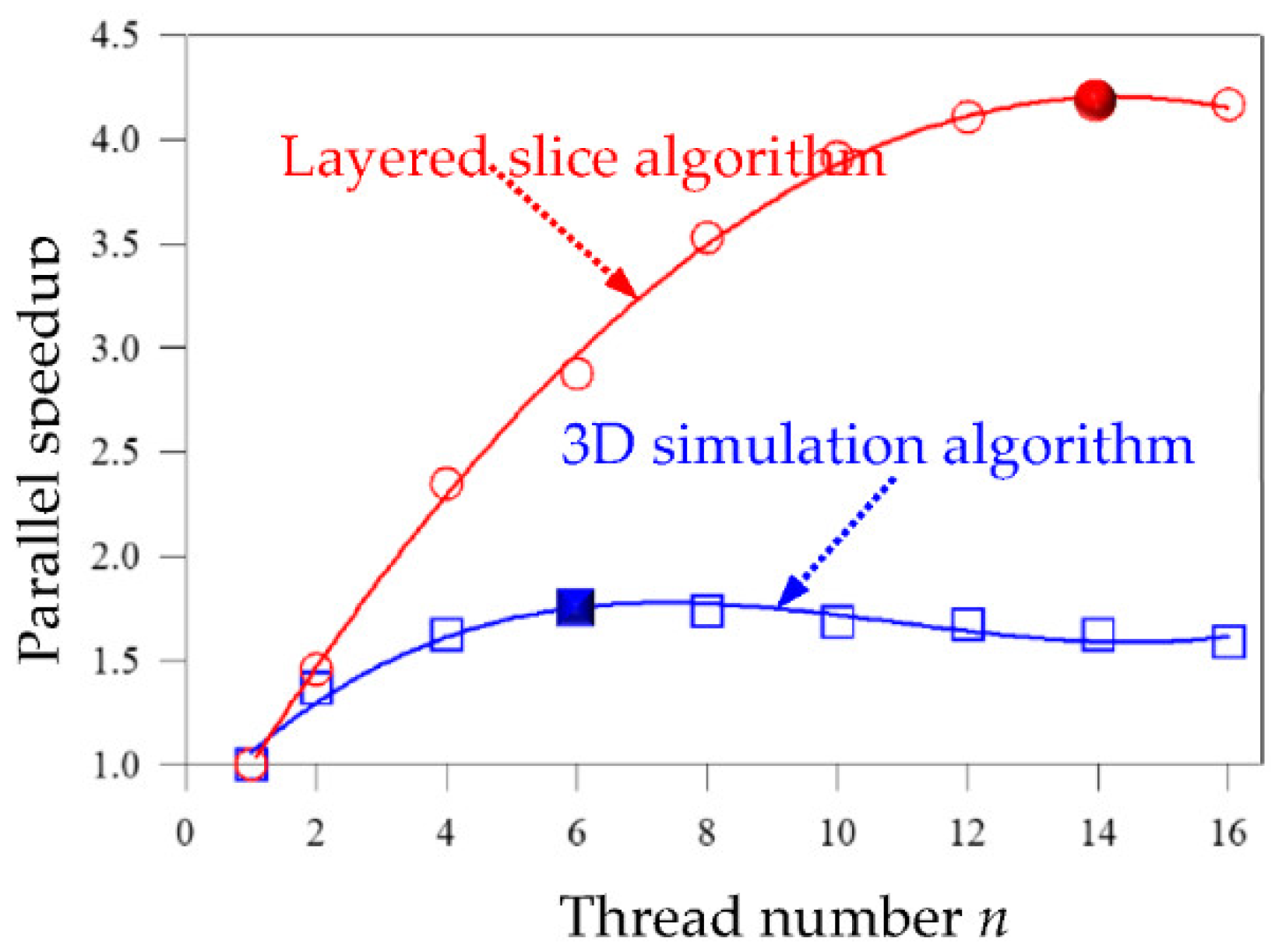
4.3.2. Parallel Performance Analysis

(1)

Qualitative analysis

Parallel computing time and parallel speedup ratio can effectively reflect the parallel performance of the algorithm. Parallel computing time mainly consists of three parts: the first is the time consumption ${\tau }_1$ of the necessary serial computing part; the second is the time consumption ${\tau }_2/n$ of the parallel computing part with n threads, and; the third is the time consumption ${\tau }_3$ of the data exchange among different threads. Thus, the parallel speedup ratio is written as:

$$S_p\left(n\right)=\frac{{\tau }_1+{\tau }_2}{{\tau }_1+\frac{{\tau }_2}{n}+{\tau }_3}$$

(34)

where (${\tau }_1+{\tau }_2$) refers to the computation time of serial computing, and (${\tau }_1+\frac{{\tau }_2}{n}+{\tau }_3$) denotes the computation time of parallel computing with n threads.

Because ${\tau }_3$ is positively related to the number of threads n, it can be expressed as:

$${\tau }_3=\alpha n$$

(35)

The value of α is determined by the amount of data exchange among different threads.

According to Equations (34) and (35), we can obtain the derivative of S_p with respect to n:

$$\frac{\partial S_p}{\partial n}=-\left({\tau }_1+{\tau }_2\right)\frac{\alpha -\frac{{\tau }_2}{n^2}}{{\left({\tau }_1+\frac{{\tau }_2}{n}+\alpha n\right)}^2}$$

(36)

It can be seen from Equation (36) that:

$$\{\begin{array}{l}n<\sqrt{\frac{{\tau }_2}{\alpha }}\to \frac{\partial S_p}{\partial n}>0\to S_p \mathrm{increases} \mathrm{with} \mathrm{the} \mathrm{increase} \mathrm{of} n.\\ n=\sqrt{\frac{{\tau }_2}{\alpha }}\to \frac{\partial S_p}{\partial n}=0 \to S_p \mathrm{gets} \mathrm{the} \mathrm{maximum} \mathrm{value}.\\ n>\sqrt{\frac{{\tau }_2}{\alpha }}\to \frac{\partial S_p}{\partial n}>0\to S_p \mathrm{decreases} \mathrm{with} \mathrm{the} \mathrm{increase} \mathrm{of} n.\end{array}$$

(37)

Compared with the traditional 3D simulation algorithm, the layered slice algorithm’s data exchange is drastically reduced. So, we can obtain:

$${\alpha }_L<{\alpha }_T\to (n_{L,\mathrm{opt}}=\sqrt{\frac{{\tau }_2}{{\alpha }_L}})>(n_{T,\mathrm{opt}}=\sqrt{\frac{{\tau }_2}{{\alpha }_T}})$$

(38)

where $n_{T,\mathrm{opt}}$ and $n_{L,\mathrm{opt}}$ refer to the optimal thread number of the traditional algorithm and the layered slice algorithm, respectively. It can be found that the value of $n_{L,\mathrm{opt}}$ is greater than that of $n_{T,\mathrm{opt}}$.

Substituting the optimal thread number $n_{\mathrm{opt}}$ into Equation (34), we obtain the maximum parallel speedup ratio:

$$S_{p,\max }\left(n\right)=\frac{{\tau }_1+{\tau }_2}{{\tau }_1+\frac{2{\tau }_2}{n_{\mathrm{opt}}}}$$

(39)

According to Equations (38) and (39), we can derive:

$$S_{pL,\max }>S_{pT,\max }$$

(40)

It means the parallel acceleration effect of the layered slice algorithm is better than that of the traditional algorithm.

(2)

Quantitative comparison

The case of periodic inlet temperature with a grid number of 600,000 is used to analyze the layered slice algorithm’s parallel performance quantitatively. Figure 16 shows the parallel speedup ratios of the traditional algorithm and the layered slice algorithm with the threads from 1~16.

It can be seen from Figure 16 that the parallel speedup ratio of both algorithms increases first, and then decreases as the number of threads increases. When the same thread numbers are used for calculation, the parallel speedup ratio of the layered slice algorithm is always greater than that of the traditional algorithm. The maximum parallel speedup ratio of the layered slice algorithm is 4.17 with 14 threads, while the traditional algorithm is only 1.75 with 6 threads. The quantitative results are entirely consistent with the above qualitative analysis.

Based on the above qualitative and quantitative analysis, we may conclude that the layered slice algorithm could gain a much higher parallel speedup than the traditional algorithm under the same conditions.

5. Conclusions

According to the structural and heat transfer characteristics of soil heat storage, a novel layered slice algorithm is proposed to efficiently and accurately calculate the soil heat storage process. Finally, through systematic and comprehensive comparison with the traditional 3D simulation algorithms, the following conclusions can be drawn:

(1)

The layered slice algorithm has a high simulation precision. For both cases of the fixed and periodic inlet temperatures, the maximum relative errors are only 0.18% and 0.19%, respectively;

(2)

The layered slice algorithm can simplify and speed up the solution process. The layered slice algorithm transforms the 3D solution process into 2D heat transfer solutions on different horizontal slices. Due to the reduction of dimensionality, the proposed algorithm has an evident accelerating effect. Compared with the traditional 3D algorithm, its calculation speed improves by 2.2~2.56 times under different grid numbers and time steps;

(3)

The layered slice algorithm has an excellent parallel characteristic. The parallel acceleration effect of the layered slice algorithm is better than that of the traditional 3D algorithm. The maximum parallel speedup ratio of the layered slice algorithm is 4.17, while the traditional 3D algorithm is only 1.75.

Due to the superior solving performance, the proposed layered slice algorithm can help the optimization design of the buried-tube heat exchangers.

References

1. Riahi, S.; Jovet, Y.; Saman, W.Y.; Belusko, M.; Bruno, F. Sensible and latent heat energy storage systems for concentrated solar power plants, exergy efficiency comparison. Sol. Energy 2019, 180, 104–115. [Google Scholar] [CrossRef]
2. Tehrani, S.S.M.; Shoraka, Y.; Nithyanandam, K.; Taylor, R.A. Shell-and-tube or packed bed thermal energy storage systems integrated with a concentrated solar power: A techno-economic comparison of sensible and latent heat systems. Appl. Energy 2019, 238, 887–910. [Google Scholar] [CrossRef]
3. Henríquez-Vargas, L.; Angel, F.; Reyes, A.; Pailahueque, N.; Donoso-García, P. Simulation of a solar energy accumulator based on phase change materials. Numer. Heat Transf. Part A Appl. 2020, 77, 443–459. [Google Scholar] [CrossRef]
4. Kursun, B. Thermal stratification enhancement in cylindrical and rectangular hot water tanks with truncated cone and pyramid shaped insulation geometry. Sol. Energy 2018, 169, 512–525. [Google Scholar] [CrossRef]
5. Dahash, A.; Ochs, F.; Janetti, M.B.; Streicher, W. Advances in seasonal thermal energy storage for solar district heating applications: A critical review on large-scale hot-water tank and pit thermal energy storage systems. Appl. Energy 2019, 239, 296–315. [Google Scholar] [CrossRef]
6. Erdemir, D.; Atesoglu, H.; Altuntop, N. Experimental investigation on enhancement of thermal performance with obstacle placing in the horizontal hot water tank used in solar domestic hot water system. Renew. Energy 2019, 138, 187–197. [Google Scholar] [CrossRef]
7. Lee, K.S. Numerical Simulation on the Continuous Operation of an Aquifer Thermal Energy Storage System Under Regional Groundwater Flow. Energy Sources Part A-Recovery Util. Environ. Eff. 2011, 33, 1018–1027. [Google Scholar] [CrossRef]
8. Fleuchaus, P.; Godschalk, B.; Stober, I.; Blum, P. Worldwide application of aquifer thermal energy storage—A review. Renew. Sustain. Energy Rev. 2018, 94, 861–876. [Google Scholar] [CrossRef]
9. Lu, H.; Tian, P.; Guan, Y.; Yu, S. Integrated suitability, vulnerability and sustainability indicators for assessing the global potential of aquifer thermal energy storage. Appl. Energy 2019, 239, 747–756. [Google Scholar] [CrossRef]
10. Li, Y.; Liu, S.; Wang, S.; Miao, Y.; Chen, B. Comparative study on methods for computing soil heat storage and energy balance in arid and semi-arid areas. J. Meteorol. Res. 2014, 28, 308–322. [Google Scholar] [CrossRef]
11. Tong, C.; Li, X.; Duanmu, L.; Wang, Z. Research on heat transfer characteristics of soil thermal storage in the non-heating season. Procedia Eng. 2017, 205, 3293–3300. [Google Scholar] [CrossRef]
12. Jahangir, M.H.; Ghazvini, M.; Pourfayaz, F.; Ahmadi, M.H.; Sharifpur, M.; Meyer, J.P. Numerical investigation into mutual effects of soil thermal and isothermal properties on heat and moisture transfer in unsaturated soil applied as thermal storage system. Numer. Heat Transf. Part A Appl. 2018, 73, 466–481. [Google Scholar] [CrossRef]
13. Pfeil, M.; Koch, H. High performance–low cost seasonal gravel/water storage pit. Sol. Energy 2000, 69, 461–467. [Google Scholar] [CrossRef]
14. Novo, A.V.; Bayon, J.R.; Castro-Fresno, D.; Rodriguez-Hernandez, J. Review of seasonal heat storage in large basins: Water tanks and gravel–water pits. Appl. Energy 2010, 87, 390–397. [Google Scholar] [CrossRef]
15. Bott, C.; Dressel, I.; Bayer, P. State-of-technology review of water-based closed seasonal thermal energy storage systems. Renew. Sustain. Energy Rev. 2019, 113, 109241. [Google Scholar] [CrossRef]
16. Umair, M.M.; Zhang, Y.; Iqbal, K.; Zhang, S.; Tang, B. Novel strategies and supporting materials applied to shape-stabilize organic phase change materials for thermal energy storage-A review. Appl. Energy 2019, 235, 846–873. [Google Scholar] [CrossRef]
17. Wang, N.; Liu, K.; Hu, J.; Wang, X. Simulation of operation performance of a solar assisted ground heat pump system with phase change thermal storage for heating in a rural building in Xi’an. In Proceedings of the IOP Conference Series: Earth and Environmental Science, Hong Kong, China, 3–5 December 2018; p. 012062. [Google Scholar]
18. Liu, C.; Xu, Z.; Song, Y.; Lv, P.; Zhao, J.; Liu, C.; Huo, Y.; Xu, B.; Zhu, C.; Rao, Z. A novel shape-stabilization strategy for phase change thermal energy storage. J. Mater. Chem. A 2019, 7, 8194–8203. [Google Scholar] [CrossRef]
19. Guo, P.; Wang, Y.; Li, J.; Wang, Y. Thermodynamic analysis of a solar chimney power plant system with soil heat storage. Appl. Therm. Eng. 2016, 100, 1076–1084. [Google Scholar] [CrossRef]
20. Zhang, L.; Xu, P.; Mao, J.; Tang, X.; Li, Z.; Shi, J. A low cost seasonal solar soil heat storage system for greenhouse heating: Design and pilot study. Appl. Energy 2015, 156, 213–222. [Google Scholar] [CrossRef]
21. Zhu, N.; Hu, P.; Xu, L.; Jiang, Z.; Lei, F. Recent research and applications of ground source heat pump integrated with thermal energy storage systems: A review. Appl. Therm. Eng. 2014, 71, 142–151. [Google Scholar] [CrossRef]
22. You, T.; Wu, W.; Shi, W.; Wang, B.; Li, X. An overview of the problems and solutions of soil thermal imbalance of ground-coupled heat pumps in cold regions. Appl. Energy 2016, 177, 515–536. [Google Scholar] [CrossRef]
23. Liu, Z.; Xu, W.; Zhai, X.; Qian, C.; Chen, X. Feasibility and performance study of the hybrid ground-source heat pump system for one office building in Chinese heating dominated areas. Renew. Energy 2017, 101, 1131–1140. [Google Scholar] [CrossRef]
24. Nouri, G.; Noorollahi, Y.; Yousefi, H. Solar assisted ground source heat pump systems—A review. Appl. Therm. Eng. 2019, 163, 114351. [Google Scholar] [CrossRef]
25. Nouri, G.; Noorollahi, Y.; Yousefi, H. Designing and optimization of solar assisted ground source heat pump system to supply heating, cooling and hot water demands. Geothermics 2019, 82, 212–231. [Google Scholar] [CrossRef]
26. Guo, D.; Zhu, J. Application of industrial waste heat to water-source heat pump. Refrig. Air-Cond. 2008, 8, 140–145. [Google Scholar]
27. Guo, M.; Diao, N.; Man, Y.; Fang, Z. Research and development of the hybrid ground-coupled heat pump technology in China. Renew. Energy 2016, 87, 1033–1044. [Google Scholar] [CrossRef]
28. Naranjo-Mendoza, C.; Oyinlola, M.A.; Wright, A.J.; Greenough, R.M. Experimental study of a domestic solar-assisted ground source heat pump with seasonal underground thermal energy storage through shallow boreholes. Appl. Therm. Eng. 2019, 162, 114218. [Google Scholar] [CrossRef]
29. Cui, P.; Diao, N.; Gao, C.; Fang, Z. Thermal investigation of in-series vertical ground heat exchangers for industrial waste heat storage. Geothermics 2015, 57, 205–212. [Google Scholar] [CrossRef]
30. Guo, F.; Yang, X.; Xu, L.; Torrens, I.; Hensen, J. A central solar-industrial waste heat heating system with large scale borehole thermal storage. Procedia Eng. 2017, 205, 1584–1591. [Google Scholar] [CrossRef]
31. Li, M.; Yu, Y. Research progress of thermal response test for GSHP system. Refrig. Air-Cond. 2010, 10, 31–34. [Google Scholar]
32. Spitler, J.D.; Gehlin, S.E.A. Thermal response testing for ground source heat pump systems—An historical review. Renew. Sustain. Energy Rev. 2015, 50, 1125–1137. [Google Scholar] [CrossRef]
33. Zeng, H.Y.; Diao, N.R.; Fang, Z.H. A finite line-source model for boreholes in geothermal heat exchangers. Heat Transf.—Asian Res. 2002, 31, 558–567. [Google Scholar] [CrossRef]
34. Lamarche, L.; Beauchamp, B. A new contribution to the finite line-source model for geothermal boreholes. Energy Build. 2007, 39, 188–198. [Google Scholar] [CrossRef]
35. Deerman, J.D.; Kavanaugh, S.P. Simulation of vertical U-tube ground-coupled heat pump systems using the cylindrical heat source solution. ASHRAE Trans. Res. 1990, 3472, 287–295. [Google Scholar]
36. Yang, W.; Shi, M. Study on cylindrical source theory based on vertical u-tube ground heat exchangers and it’s application. J. Refrig. 2006, 27, 51–57. [Google Scholar]
37. Lee, C.K.; Lam, H.N. Computer simulation of borehole ground heat exchangers for geothermal heat pump systems. Renew. Energy 2008, 33, 1286–1296. [Google Scholar] [CrossRef]
38. Li, Z.; Zheng, M. Development of a numerical model for the simulation of vertical U-tube ground heat exchangers. Appl. Therm. Eng. 2009, 29, 920–924. [Google Scholar] [CrossRef]
39. Yv, C.Y. Research on Heating System of Solar Energy Inter Seasonal Heat Storage Composite Ground Source Heat Pump for Agricultural Greenhouse. Master’s Thesis, Beijing Institute of Petrochemical Technology, Beijing, China, 2020. [Google Scholar]
40. Sun, D.; Wang, L.; Xu, J.; Lu, X. Research and Application of Temperature Stratification Model for Seasonal Water Tank Heat Storage. Acta Energ. Sol. Sin. 2014, 35, 291–298. [Google Scholar]
41. Tao, W. Modern Development of Computational Heat Transfer; Science Press: Beijing, China, 2000. [Google Scholar]
42. Peng, X.; Chen, G.; Yu, P.; Zhang, Y.; Guo, L.; Wang, C.; Cheng, X.; Niu, H. Parallel computing of three-dimensional discontinuous deformation analysis based on OpenMP. Comput. Geotech. 2019, 106, 304–313. [Google Scholar] [CrossRef]
Figure 1. The physical model for soil heat storage system.
Energies 15 03743 g001
Figure 2. The simplified physical model for soil heat storage system and the corresponding boundary conditions. (For convenience, this figure shows all the four straight pipes in the middle. Their real relative positions refer to Figure 1).
Energies 15 03743 g002
Figure 3. Geometric relationship on both sides of the interface e.
Energies 15 03743 g003
Figure 4. One-dimensional grid system for the interior of the tube.
Energies 15 03743 g004
Figure 5. The unstructured quadrilateral grid on the horizontal section for the generalized heat-storage body.
Energies 15 03743 g005
Figure 6. 3D grid system for the generalized heat-storage body.
Energies 15 03743 g006
Figure 7. Evolution of temperature with time at observation points calculated by the Fluent software and the traditional 3D simulation algorithm under thermal storage condition.
Energies 15 03743 g007
Figure 8. Temperature change at three different points near the U-tube for the case of fixed inlet temperature.
Energies 15 03743 g008
Figure 9. Comparison of temperature fields computed by different algorithms at vertical section of x = 0 for the case of fixed inlet temperature.
Energies 15 03743 g009
Figure 10. Comparison of temperature fields computed by different algorithms at horizontal sections of z = −11.5 m and z = −91.5 m for the case of fixed inlet temperature.
Energies 15 03743 g010
Figure 11. Temperature change at three different points near the U-tube for the case of periodic inlet temperature.
Energies 15 03743 g011
Figure 12. Comparison of temperature fields computed by different algorithms at vertical section of x = 0 for the case of periodic inlet temperature.
Energies 15 03743 g012
Figure 13. Comparison of temperature fields computed by different algorithms at horizontal sections of z = −11.5 m and z = −91.5 m for the case of periodic inlet temperature.
Energies 15 03743 g013
Figure 14. Parallel computing process of the traditional 3D simulation algorithm.
Energies 15 03743 g014
Figure 15. Parallel computing process of the layered slice algorithm.
Energies 15 03743 g015
Figure 16. Parallel speedup ratio of layered slice algorithm and 3D simulation algorithm with different thread numbers.
Energies 15 03743 g016