1. Introduction
Energy transition is expected to be accelerated, driven primarily by an increase in the share of renewable energy sources (RES) in the global energy mixture. From a technical aspect, this is strongly related to developments in the fields of energy storage [
1] and distributed energy resources (DERs) [
2], including cogeneration and trigeneration technologies. In this direction, local energy systems designed to utilize various combinations of novel energy technologies are of great interest. Special focus is given to their evaluation and the replicability of the most promising among them. A crucial and challenging prerequisite to come to meaningful conclusions is the accurate and reliable representation of these systems through dynamic modeling.
Over the last few years, numerous studies have developed dynamic models of RES-based local energy systems in order to assess the energy performance of their current design or proposed alternative scenarios [
3]. On top of that, energy management strategies that enable optimal synergies between interacting energy assets have been proposed and evaluated [
4].
Systems that incorporate solar thermal energy production and biomass combustion for heating, domestic hot water (DHW) and cooling, through absorption refrigeration, have been analyzed through dynamic models [
5,
6,
7]. In [
8,
9,
10], the authors investigate the the performance of combined heat power (CHP) production with integrated Organic Rankine Cycle (ORC) systems for residential or industrial waste heat recovery applications. More specifically, dynamic models with the use of the equation-based language Modelica have been proposed in [
11,
12]. Research in this field also focuses on applications of solar cooling and combined cooling, heat and power (CCHP or trigeneration) to increase system energy efficiency [
13,
14,
15,
16]. Regarding thermal energy storage (TES) systems, authors in [
17,
18] investigated their effect on heating and cooling applications covered by RES.
Furthermore, a considerable amount of research activity is associated with the area of dynamic simulation of grid-connected or islanded microgrids [
19,
20]. A research subject of special interest is also the performance of cooperative photovoltaic (PV) and ORC units, which is presented in [
21,
22,
23]. The effect of battery energy storage in decentralized RES power generation is also studied in recent literature [
24,
25]. Focus is also given to the development of proper battery component models with sufficient accuracy, capable to integrate with the broader system models. In solar applications, the widely approved method of equivalent electric circuit, first proposed in [
26], is the most common choice for battery modeling [
27]. Furthermore, although the effect of battery chemistry on system performance is an issue of special concern, attention is mainly given to the financial comparison of the different types [
28,
29,
30,
31].
This study focuses on the investigation of a LES, in which energy is generated by solar thermal collectors, a biomass boiler, a PV system and an ORC unit serving the demand of heating, DHW, cooling and electricity of a student residence building complex in Xanthi, Greece. For that purpose, a multidomain dynamic system model has been developed, incorporating detailed submodels of each energy asset. Model development has been implemented in Modelica language within Dymola software. To strengthen the profitability gained from the system model, a validation process has been performed, in which simulation results have been compared against measured data. The validated model is then used for the evaluation of system performance, the definition of technical barriers and the comparison of alternative design and operation scenarios. The solutions examined include energy-saving measures and the replacement of the existing lead–acid battery system with an equivalent, in terms of energy capacity, lithium-ion which is known for its higher energy density [
32].
The main contributions of this research are:
Dynamic modeling of energy system components in Modelica language, in comparison with most available open-access studies that use commercial or proprietary software, including the equivalent circuit model of a nickel manganese cobalt oxide lithium-ion battery cell.
The integration of all components into a system-level model following a unified multidomain approach, and a subsequent validation procedure against measured field data.
The proposal of seven measures in the thermal grid of the system under study, which increase the contribution of solar thermal field in the heating and DHW energy supply from 12.64% to 37.26%, as well as two further measures in the electrical grid that lead to a 4.9% rise in PV generation.
In a nutshell, the followed methodology results in the evaluation of the proposed measures as capable to lead to an enhanced system energy performance.
This paper is structured as follows:
Section 2 imports the methodology followed throughout this work.
Section 3 provides a description of system configuration and energy management priorities. All stages of the model development are described in
Section 4. The scenarios under examination are defined in
Section 5 and the results are presented in
Section 6. Finally, the conclusions of this work are consolidated in
Section 7.
2. Methodology
The followed methodological framework aims to examine in detail a trigeneration system through extensive and numerous parametrically studied dynamic simulations. The analysis aims to enhance system operation in terms of energy efficiency and formulate a report on best practices among interacting energy vectors.
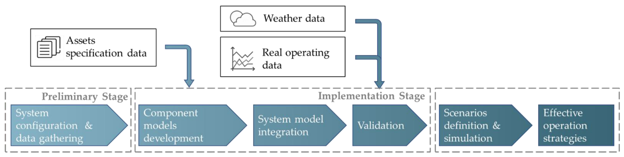
The process stages of the overall methodology are depicted in
Figure 1 in a diagram form. As the validity of the proposed operation strategies relies on the accuracy of the energy system representation, a comprehensive validation procedure has been incorporated.
Methodology consists of three stages. The preliminary stage involves the accurate definition of the system which will be represented, taking into account all relevant energy assets, their configuration, the overall topology and the necessary control systems. The implementation stage follows, where the model development takes place. The first step includes the development of accurate models for the representation of each individual part of the complete system setup. In this step, the collection of assets’ design and operating data plays an important role in model accuracy. Moreover, as already mentioned, the involvement of multiple power transactions occurs and as a result, the coupling of many different submodels is required. In the final step of this stage, implementation moves forward with the model validation against available measured data. This stress test of the system dynamic model is followed by the evaluation stage. Alternative design and operation scenarios, based on examined possible measures, are proposed and simulations are conducted. In the final step, the quantities of RES energy production and their share in the local energy mixture are compared to arrive at conclusions regarding optimal system performance. As a result of the methodological framework described, a deep and solid perspective of system operation is achieved.
3. System Description
The system under study is located in Xanthi, Greece and serves energy demands for heating, cooling, DHW and electricity of the Democritus University of Thrace local student residencies. The building complex consists of 8 buildings that include 778 student rooms, an amphitheater and a restaurant. The present section includes a brief description of the system configuration and the available assets along with the main energy management strategy. For a detailed description of the system, the reader is referred to relevant works [
33,
34].
3.1. Energy Assets Overview
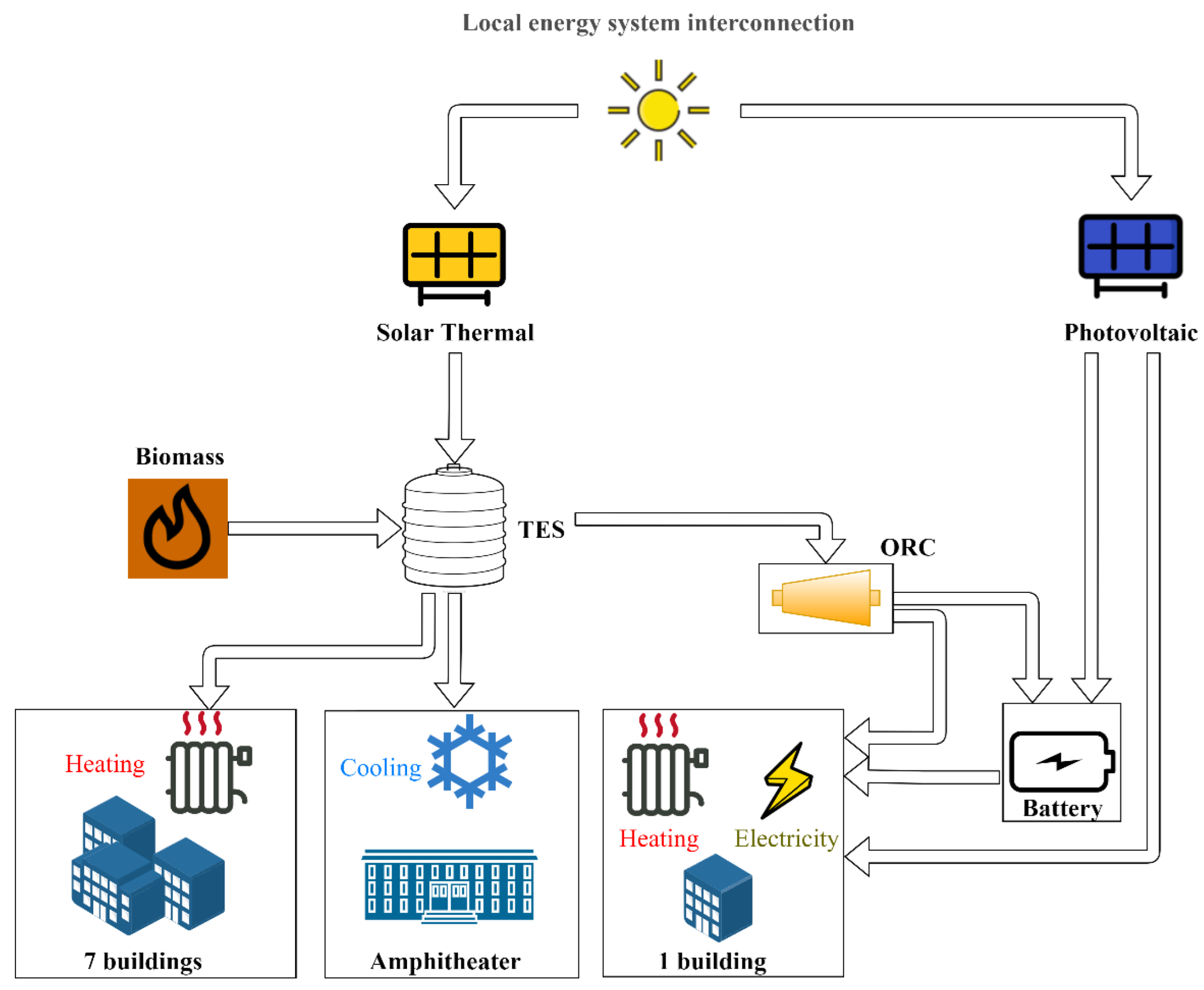
The energy system involves several assets from different energy domains coupled together and is depicted in
Figure 2. The system can be considered as of two main integrated subsystems, namely the thermal grid which covers the heating and DHW demand of the 8 buildings as well as the cooling demand of the amphitheater, and the electrical grid which covers partially the loads of a single building. Reference to the two grids is made separately throughout the manuscript, despite their interconnection through an ORC unit.
The thermal grid can be considered as an application of trigeneration or CCHP, exploiting solar and biomass as primary energy sources. A TES system that includes hot water tanks of a total volume of 49 m
3 offers significant heat storage capacity, and therefore temporal flexibility. The heat generated by the system covers the annual heating demand of most of the residences’ buildings. The average annual thermal energy delivered to the building complex is approximately 1900 MWh. Moreover, an absorption refrigeration network covers the cooling demand of an amphitheater for approximately one month during the summer months. For the operation of the absorption chiller, the average thermal energy consumption is 45 MWh
th/y, 94% of which is delivered by the solar field. With the provided seasonal coefficient of performance (SCOP) value of 0.57, this is equivalent to a cooling demand of 25.6 MW
c/y. An ORC system of 7 kW
e capacity is also integrated into the same system, receiving heat through the connection with the biomass boiler exit point and providing electricity to the local electrical grid. The key technical parameters of the aforementioned assets are listed in
Table 1.
The local electrical microgrid includes a PV installation, a lead–acid battery system and an ORC unit, powered by the thermal grid, that supply the electrical loads of the common spaces of a single student residences building and an electric bicycle charger through 4 separate power converters. It should be noted that the ORC system is recently installed and is not yet operational. Technical specifications of the grid assets are presented in
Table 2. In a previous study of the system, the annual electric load of the system has been estimated at 8 MWh/y, whereas the annual electricity generation at 73 MWh/y, which is the 3.2% of the total complex electricity demand [
35]. The rest of the demand is served by a connection with the external grid.
3.2. Energy Management Overview
In this section, the priorities of energy flows during operation are described, according to the existing control schemes, design operating conditions and technical limitations of power generation, storage and conversion assets.
In the thermal grid, solar energy is transferred to a 20% propylene glycol solution, through four independent sets of flat-plate solar collectors (loops). In each loop, a water flow is then heated through a plate heat exchanger, flowing to the TES system, which consists of hot water storage tanks. Hot water reaches the biomass boiler and is afterward supplied to the building complex heating distribution system or the amphitheater cooling system during the summer months. If necessary, the water temperature is increased by the boiler up to 90 °C. Otherwise, the boiler may remain turned off. Physical quantities, such as temperature and pressure, are monitored at different system points, enabling complex control schemes of pump actuators and three-way valves. These real-time measured data, that lead to the definition of operating strategies of the energy system, are collected in a smart-decision hub of the system.
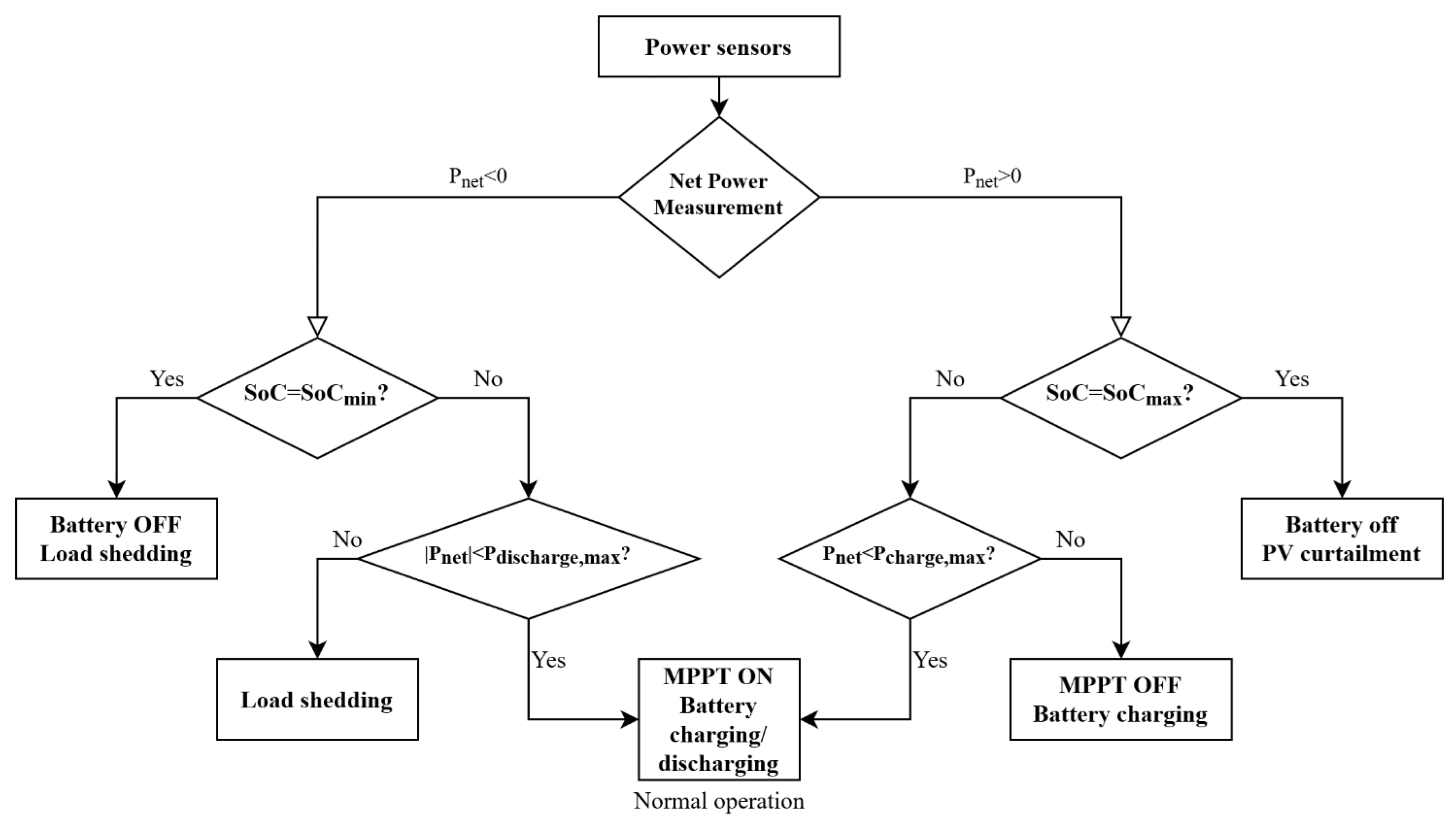
The energy management rules applied to the electrical microgrid, in this study, are simpler due to its lower complexity. PV inverters ensure that maximum available power is injected into the microgrid through a maximum power point tracker (MPPT) algorithm [
36] when the battery is not fully charged. If the power generation exceeds the load demand, the battery charging process is taking place, while in the opposite condition, the battery system provides the power deficit between PV generation and load consumption. Battery daily depth of discharge (DoD) is always kept below its safety limit (defined at 25% for the specific application by the manufacturer). When DoD approaches this value, ORC generation is used as a backup power source for the microgrid. This way, battery operation is extended and therefore energy storage of surplus PV power that otherwise would be curtailed is enabled. However, ORC’s low efficiency results in an electric power generation of 7 kW
e after the extraction of more than 100 kW
th from the thermal grid. As a consequence, for the consideration of ORC synergetic operation with the thermal and electrical grids, whether its operation is dependent on solar or biomass energy must be taken into account. The logic rules described above are depicted in a flow diagram in
Figure 3.
4. Model Development
System models are designed in Dymola software using Modelica, an equation-based modeling language. One of its basic characteristics is being object oriented and, as such, it supports bottom-up system design. More specifically, the followed approach builds larger system models based on the interconnection of individual components. That way, complex non-linear physical systems can be solved precisely in the time domain, through a set of differential and algebraic equations. The next few paragraphs present the developed models and provide important insight into the modeling process.
4.1. Meteorological Data
Prior to model development, the provision of accurate meteorological data must be secured since they are an essential input to proceed with model simulation. The result of the validation procedure relies as well on the utilization of weather data for the specific days under examination. Furthermore, the accuracy of the weather data directly affects the results of the validation process, an inevitable effect that should be kept in mind during the evaluation of the results. Thus, for the validation procedure and the scenario evaluation stage, SARAH-2.1 [
37] datasets have been used, where data are made available through satellite observations.
4.2. Component Modeling
4.2.1. Solar Collector
A case-specific model has been developed for the entire solar field, which consists of four loops. Each loop consists of two connected configurations. The first configuration consists of 4 collectors connected in series and 20 in parallel. Additionally, the second of 5 collectors connected in series and 20 in parallel. The solar collector type is flat-plate and no shadow effects take place in order to be considered. The modeling equations of the collector are derived from the literature [
38].
More specifically, solar collection efficiency, defined as the ratio of the useful gain over some specified time period to the incident solar energy over the same time period, and energy balance can be combined in the equations:
where the term
represents the useful energy gain in W,
is the collectors’ clean area in m
2,
denotes the solar irradiance on a tilted plane in W/m
2,
denotes the dimensionless heat removal factor, (τα) represents the dimensionless transmittance-absorptance product of the collector,
is the collector overall loss coefficient in W/(m
2 °C),
is the collector fluid entering temperature (in °C),
is the ambient temperature (in °C),
is the collector mass flow rate (in kg/s),
is the specific heat of the collector fluid (in J/kgK) and
is the fluid exit temperature (in °C)
The incidence angle modifier is calculated from the equation:
where b
0 represents the dimensionless incidence angle modifier coefficient and θ represents the instantaneous incidence angle.
In order to properly model the complex configuration of the high number of collectors, in series and parallel, certain modifications have been implemented in the Buildings library default solar thermal collector model.
4.2.2. Organic Rankine Cycle System
In order to have an increased RES power generation and energy conservation, an ORC system installation has been deployed. Concerning the operating temperature range of the available hot water, and in respect of low environmental impact specifications (Low Ozone Depletion Potential—ODP and Global Warming Potential—GWP), as imposed by EU legislation [
39], R245fa (pentafluoropropane) has been selected as the working fluid. Technical specifications of the installed ORC system, as provided by the manufacturer, are described in
Table 3.
Thermocycle [
40] and ExternalMedia [
41], two open-source Modelica libraries focused on thermodynamic cycles, have been used for the model development. Thermocycle provides the background to simulate thermodynamic cycles, including ORC. ExternalMedia includes embedded libraries, such as CoolProp [
42] and RefProp [
43] with thermodynamic properties of non-conventional working fluids. The states of the thermodynamic cycle, used for the simulations, are listed in
Table 4.
The following control mode operation is assumed by the model. ORC generator is turned on under only certain operating conditions, i.e., whenever battery DoD overcomes the maximum allowable threshold (25% specification for the specific battery) and when microgrid net power turns negative, which would otherwise lead to load shedding. The control block of the model adjusts the variable of the expander filling factor (ff), in order to control the value of the output variable, which is the generated power, at the desired level.
The model set of equations:
where
is the mass flow rate entering the expander in kg/s,
is the fluid density in kg/m
3,
is the superheated vapor temperature in °C,
is the swept volume in m
3,
is the exiting vapor specific enthalpy in J/kg,
is the superheated vapor specific enthalpy in J/kg,
is the isenthalpic exiting vapor specific enthalpy in J/kg,
is the dimensionless isentropic efficiency of the expander,
is the net output power in W,
is the dimensionless electromechanical efficiency and
is the pump electric consumption in W.
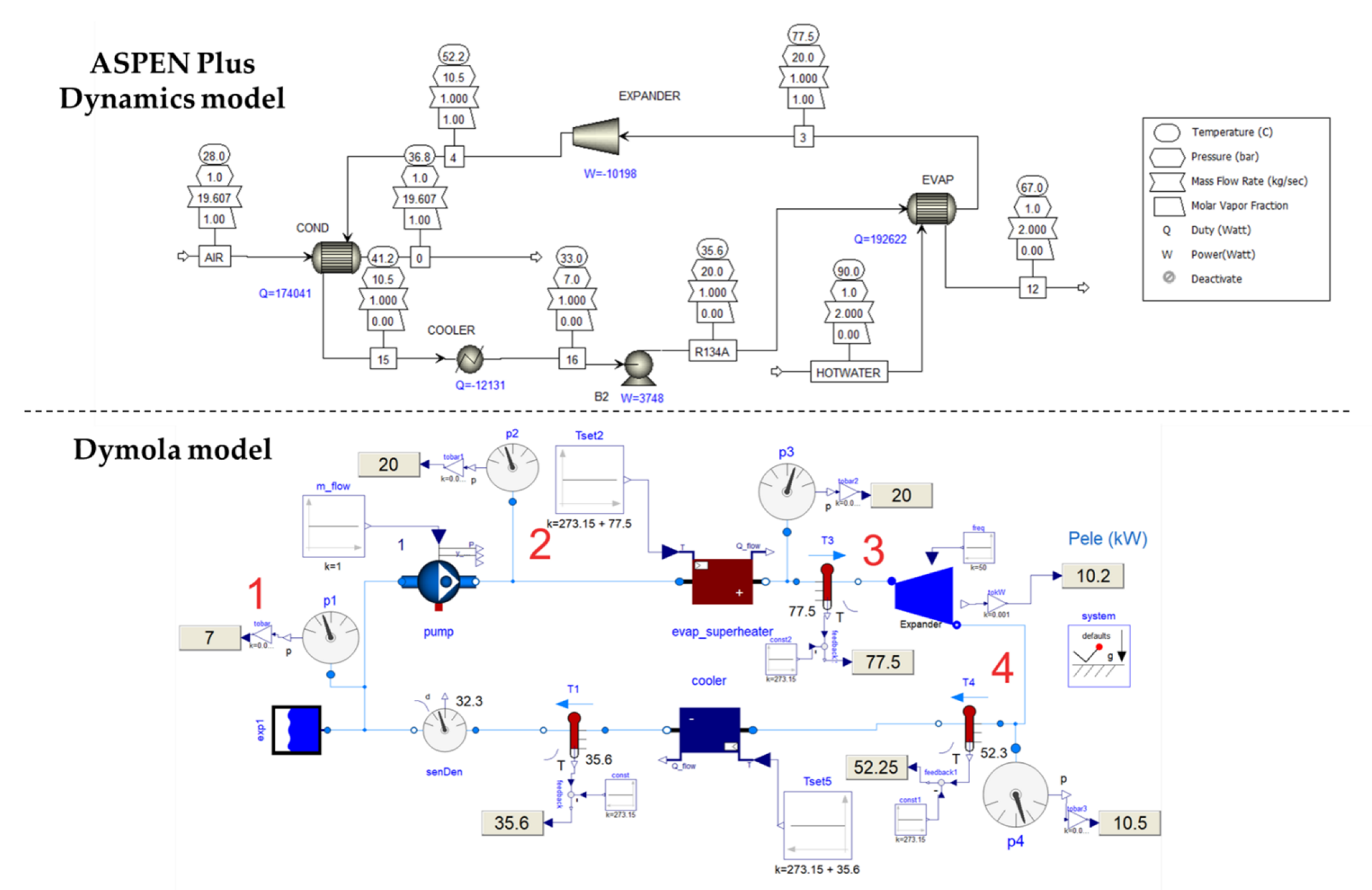
The developed model has been verified against simulation results of ASPEN Plus Dynamics, specialized software for combustion processes and thermal power plants. A reference case of an ORC system of 10 kW
e has been considered. For the cycle under examination the refrigerant R134a is the working fluid. The cycle thermodynamic states are presented in
Table 5. To verify the model’s accuracy, the expander output power value of the two software has been compared and the deviation is below 0.02% (i.e., 2 W). The simulation results, including all of the system design points compared, are depicted graphically in
Figure 4.
4.2.3. Absorption Chiller
Absorption chillers are often utilized for the exploitation of hot water for cooling purposes. In this application, during the summer months, hot water from the hybrid system is supplied to the chiller’s generator providing the necessary heat to generate steam in the absorption cycle. Whenever the TES system water temperature is below the chiller hot water specification threshold of 65 °C, the biomass boiler is turned on. The main parameters are included in
Table 6.
Integration with the upper-level model can be succeeded through three independent flow networks, i.e., hot water, cooling tower water and chilled water. Based on the chiller and cooling tower datasheets, a polynomial fit approach has been followed to calculate the heat flows of the evaporator, condenser, generator and absorber depending on each flow’s input temperature and part-load ratio. The second order polynomial functions used are:
where
is the water entering temperature from the cooling tower in °C,
is the dimensionless generator heat input modifier with dependence on
,
is the dimensionless part-load ratio,
is the dimensionless pump electric input ratio with dependence on
and
,
,
,
,
are the extracted polynomial coefficients.
The equation set for the calculations of chiller energy transactions is:
where
is the necessary heat flow rate to reach the chilled water temperature setpoint in W,
is the mass flow rate of the chilled water in kg/s,
is the specific enthalpy of the chilled water in J/kg,
is the temperature setpoint of the chilled water in °C,
is the inlet temperature of the chilled water in °C,
is the heat flow rate at the evaporator in W,
is the nominal heat flow rate at the evaporator in W,
is the pump power in W,
is the nominal pump power in W,
is the dimensionless heat input ratio,
is the dimensionless nominal coefficient of performance,
is the heat flow rate at the generator in W,
is the heat flow rate at the condenser in W and
is the heat flow rate at the absorber in W.
The model uses performance curves equivalent to the reliable EnergyPlus model (Chiller:Absorption:Indirect). Certain adjustments have been made, only focusing on the interconnection capability with the hot water stream from the biomass boiler, so that the amount of heat removal is accurately calculated considering chiller dynamic effects.
4.2.4. Lead–Acid Battery Cell
To proceed with the representation of the battery system, a dynamic model of the battery cell has been developed. This way, accurate predictions of battery pack terminal voltage, SoC and temperature are provided by the simulation, enabling operation in compliance with battery health and safety protocols.
The electrical model is based on the widely used equivalent circuit model (ECM) method, which has been described thoroughly in [
26,
44]. Each manufacturer-specific battery cell type differs in terms of operating conditions as a result of its own chemistry properties; thus, it has a unique set of parameters and needs special handling in the modeling process. Because of this, battery cell models need to be specialized for the specific battery type. The existing battery system consists of flooded type tubular-plated lead–acid batteries known as OPzS, whilst the one considered as a possible replacement in the case under examination consists of lithium-ion battery cells; therefore, two different models have been developed. First, the model developed for the OPzS battery cell is presented.
As no experimental data were available, the modeling technique that has been followed is datasheet based and is based on a methodology described in [
45], to obtain a valid and accurate model for the specific application. An ECM of the proposed topology, shown in
Figure 5, is considered to capture the transient response of complex internal chemical processes. The circuit elements are introduced as parameters with values derived from mathematical expressions obtained by curve-fitting or one-dimensional look-up tables. Circuit parameters are considered to only be dependent on SoC and current values over time. This way, for a known input time series of power (and therefore current) values the battery SoC and terminal voltage response are given as outputs as time evolves. A simplification has been made assuming the same values of polarization resistance have been used for both charging and discharging processes. Since, as described in
Section 3.1, each battery pack consists of three parallel strings of 24 cells in series, proper scaling transformations are implemented to represent the battery pack configuration.
The extracted equations for the calculation of OPzS parameter values during battery operation are:
where
is the cell capacity,
is the cell current, OCV denotes the open circuit voltage and R
bd is the part of polarization resistance that depends on the SoC.
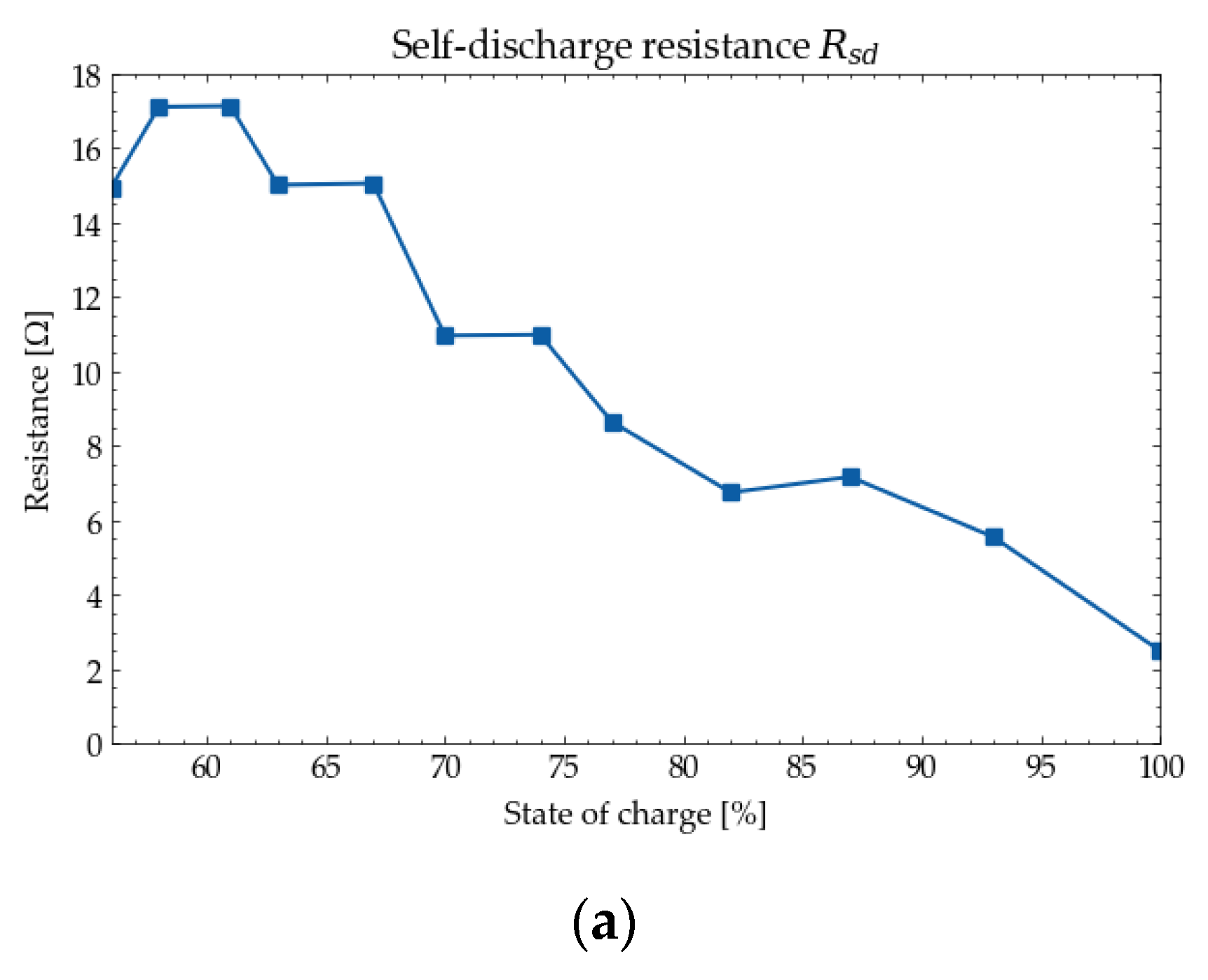
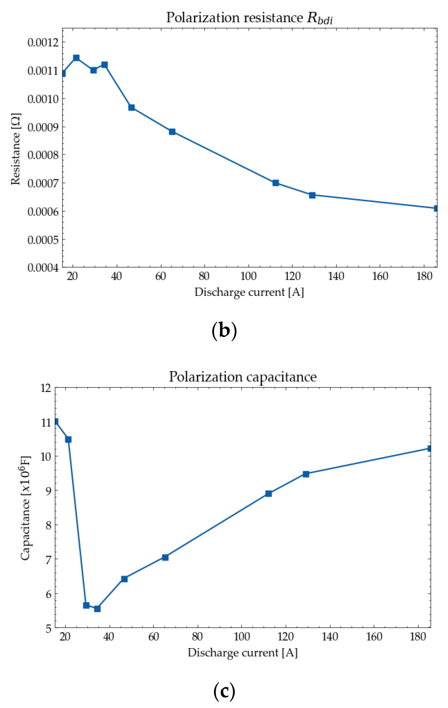
The extracted one-dimensional look-up tables for the calculation of parameter values are presented in
Figure 6.
4.2.5. Lithium-Ion Battery Cell
For the Li-ion battery cell modeling, the model topology and the parameter estimation techniques implemented are described in detail in [
46,
47]. The model focuses on accurately calculating the terminal voltage and SoC of each cell of the battery system configuration, based on the instantaneous power extracted to (discharging) or received by (charging) the connected electrical grid. Battery voltage response evolves with a nonlinear behavior when electric charge is transferred through battery terminals, and this is due to complex electrochemical phenomena (polarization–diffusion, double layer). These transient phenomena, related to the nonlinearity of voltage response, are captured by a number n
RC of parallel resistor–capacitor (RC) branches. This number is decided by the specific battery application, required accuracy and available computational resources. A resistance connected in series (R
0) represents the instantaneous voltage drop, while open-circuit voltage (OCV or E
m) reflects the available internal energy. All of the above model parameters are dependent on SoC, temperature and current and therefore their values are extracted for varying external conditions from look-up tables made available from specified test measurements.
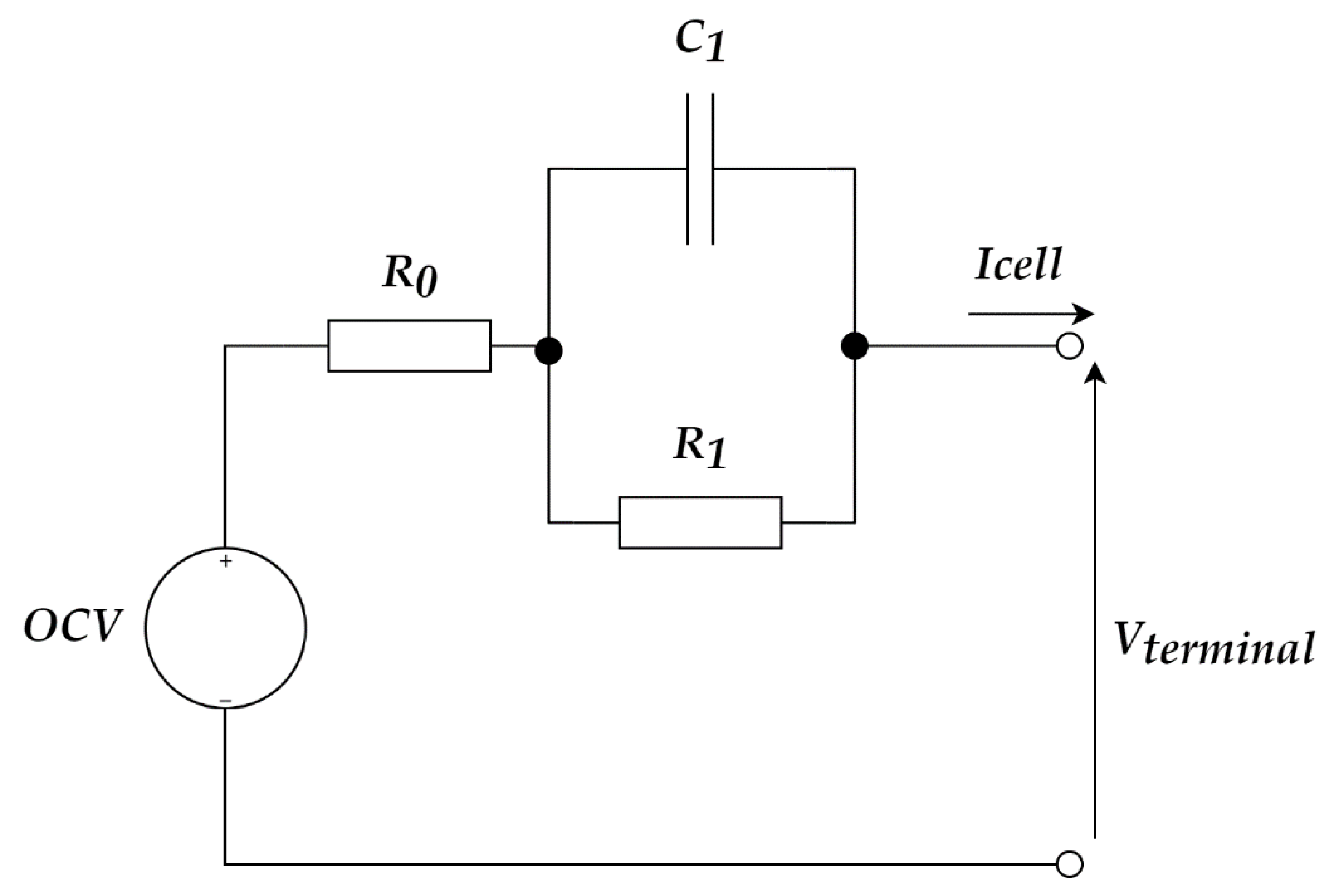
The current study focuses on a solar off-grid battery application and, therefore, the number of parallel RC branches is decided to be 1, since adequate accuracy is secured for the expected current dynamic response. On top of that, model efficiency in terms of computational complexity decreases significantly. The topology of the model with a single RC branch is depicted in
Figure 7.
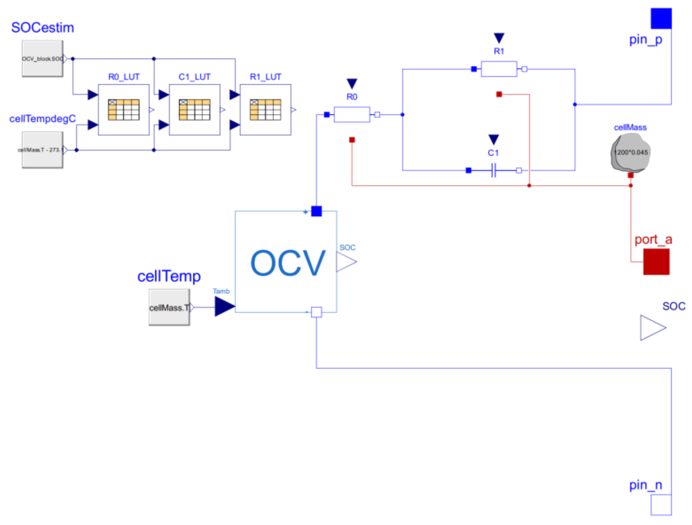
The cell model developed originally in Modelica is graphically shown in
Figure 8. The developed battery pack model supports the automated integration of any possible cell configuration. For n
RC = 1, the model uses Equation (15) for SoC estimation and the following set of equations:
where
and
are the battery cell mass in kg and specific heat in J/(kg∙K), respectively.
Modeling of battery cell capacity dependency on temperature is given in
Table 7.
To proceed with the parameter estimation stage, data from pulsed current discharge test at specific SoC breakpoints are necessary, following a constant current–constant voltage (CC-CV) full charging process. For this study, data made available in [
48] for a 18650 NMC battery cell have been used. Due to battery cell chemistry variations, each parameter set is actually the specific battery fingerprint and determines the model accuracy. For the implementation of the parameter estimation stage, MATLAB Simulink Design Optimization toolbox is utilized. The procedure is repeated in three different temperatures, enabling model dependency on thermal operating conditions and, thus, leading to accurate adjustments of critical quantities, such as available capacity or maximum allowed current. The results of the extracted parameters are presented in
Figure 9. The percentage values of the sum squared error (SSE) as a percentage of cell nominal voltage are listed in
Table 8.
4.2.6. Power Converters
Power converters (inverters) are used for the connection of PV, ORC and battery systems with the AC side of the local microgrid. Custom exclusive models have been developed, where the quasi-stationary theory described in [
49] has been followed for the AC side. AC signals are expressed as phasors with the use of Modelica Standard Library components. Since the grid is in islanded mode, each inverter plays a different role and this must be taken into account by the model. The battery inverter acts as a voltage-source control (V-f inverter) and PV and ORC inverters act as a current-source control (P-Q inverter).
4.3. System Modeling
4.3.1. Thermal Grid
The developed system model of the thermal grid is presented in
Figure 10. As can be seen, each solar loop has its own pump actuator block. This block ensures that the mass flow rate becomes zero in the case of negligible useful solar energy or collector temperature below 25 °C, in order to minimize heat losses to the environment. The collected energy is transferred in each solar field loop from the heated water-glycol solution to the water circuit, through a heat exchanger. Moreover, control blocks are used to decide the tank charge and discharge strategy, based on system temperatures and load conditions. The biomass boiler is used as a backup heating unit, to provide a high enough temperature for the distribution system, when needed. The terminal units, as well as the absorption chiller and the ORC system, remove an amount of thermal energy from the circulating water, which is calculated from each subsystem load demand. Additionally, the weather data are used to compute all the necessary external conditions that are used as inputs for each component model. The heating system covers the demand of eight buildings for the entire winter period (October to April) while cooling demand refers only to approximately one month of operation of the amphitheater during summer. Electricity generation through the ORC system covers a relatively low load (common loads of a single building) supplementarily to the existing PV system.
4.3.2. Electrical Grid
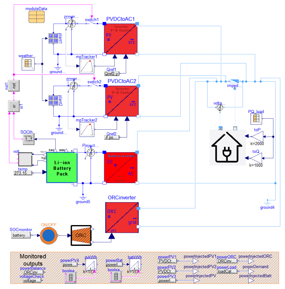
The dynamic model developed for the Kimmeria islanded power supply system is presented in
Figure 11. The increased complexity of such a group of equations increases the simulation run time significantly. System response yields from a phasor analysis that was implemented in the 3-phase AC branch between power generation and load. On top of that, a simple operation control algorithm has been developed focusing on the proper charging and discharging process of the battery. The algorithm ensures operation within the specified safety limits of voltage (between 1.9 V and 2.1 V per cell) and maximum daily DoD (below 25%) as described by the manufacturer. The energy management priorities are explained in more detail in
Section 3.2. For the PV control system, a necessary MPPT algorithm has been utilized. ORC operates as a backup generator to ensure the safe operation of the battery system.
4.4. Model Validation
4.4.1. Thermal Grid
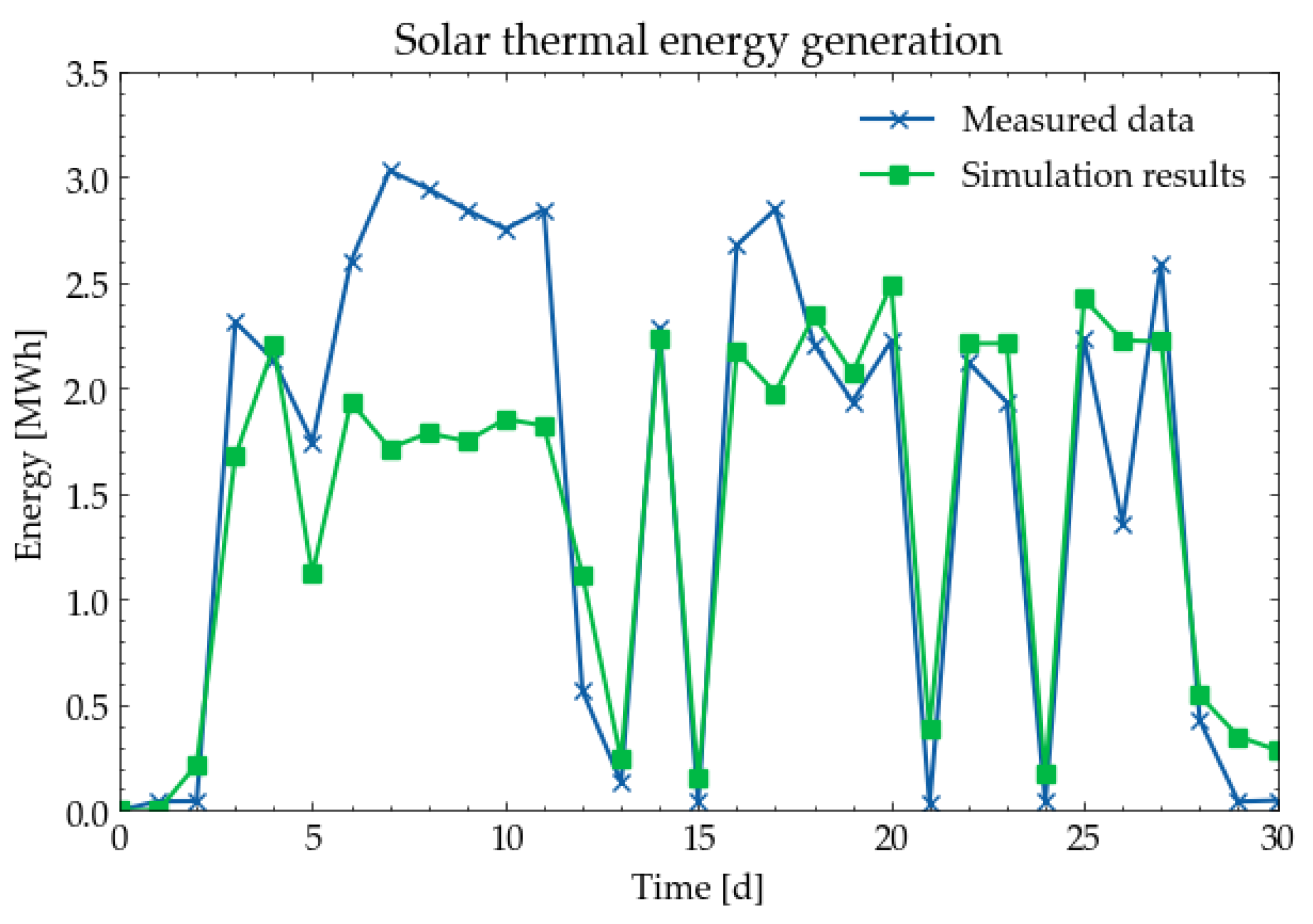
To validate the thermal grid model, simulation results have been compared against available measurements of the energy generated by the hybrid system of the solar field and the biomass boiler. The time period selected for the validation process is the first 30 days of October 2019, where measured data are available. Since weather data from the period under examination are not available, data from SARAH-2.1 have been used as input, which is a key aspect of the validation process. Hence, deviation from actual temperature and irradiation values can arise as an obstacle on certain days, affecting the accuracy of the simulation results. To overcome the effect of daily value deviations on the result, the amounts of energy produced over the entire month are compared. Measured heating load demand time series from the period under examination is also used as input for the developed model.
In
Figure 12, simulation results of energy produced by the solar field are compared against the measured values. The maximum daily error reaches 1.3 MWh on day 7. The total energy produced by the solar field over the 30 days of October is estimated at 47.8 MWh. The absolute estimation error is 2.2 MWh (or 4.4%). This deviation could be explained by the weather input data used, since data extracted from the satellite observations might deviate from the actual conditions and lead to an underestimation of the available solar irradiance, mainly between days 5 and 12.
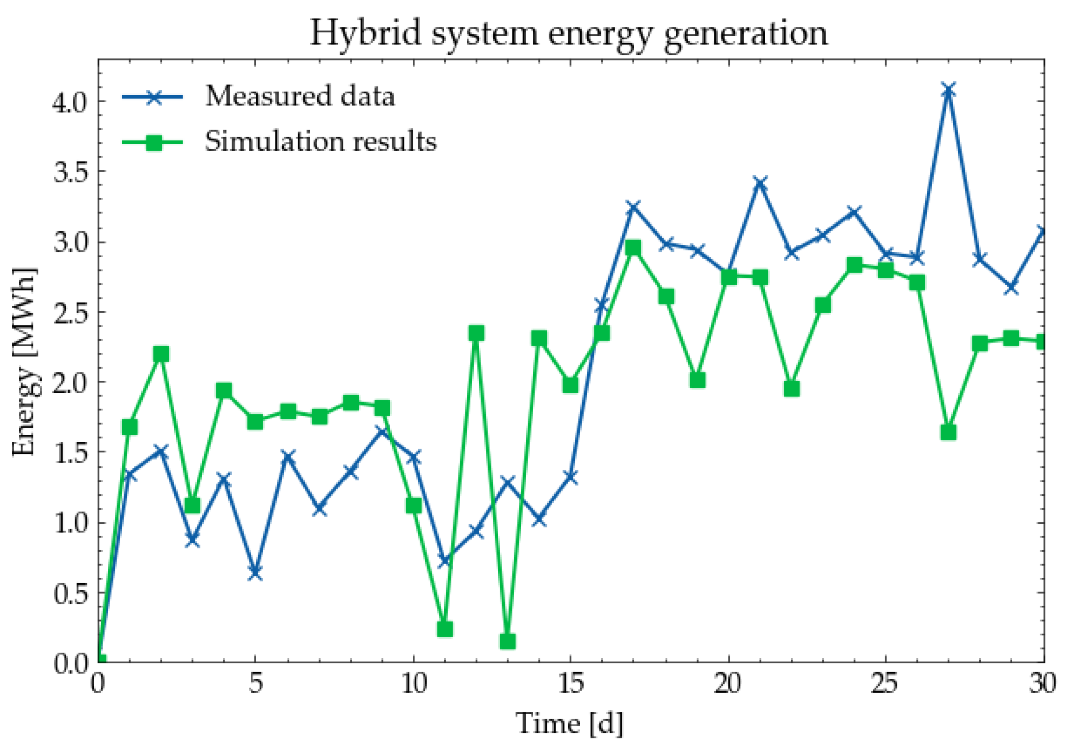
In
Figure 13, simulation results of the energy produced by the entire hybrid (solar/biomass) system are compared against the measured values. Again, the curves represent the evolution of aggregated daily energy values. The total energy production from 1 October until 30 October is estimated at 63 MWh and the estimation error is 3.3 MWh (or 5.0%), whereas the maximum daily error reaches 2.4 MWh on day 27. Deviations, in this case, can also be explained by a possible inconsistency between actual and used weather data.
It should be highlighted that the available measurements have been received by heat meters installed in specific system points, resulting in the necessity of certain clarifications about the conducted comparisons. More specifically, heat meters measuring the generated solar thermal energy are installed in the solar field entry and exit points. This means that heat losses due to the heat distribution grid (piping length is 150 m) are neglected. On the other hand, regarding hybrid system measurements, since heat meters are installed in the entry and exit point of the system as well, heat losses to the environment are taken into account.
4.4.2. Electrical Grid
The validation process of the electrical grid draws on the same approach as in
Section 4.4.1, leading to a comparison between measured data and simulation results of the energy generated by the PV installation. In this case, the period examined is June 2020, whereas the weather data are also obtained by SARAH-2.1 and the load demand time series is received from measurement equipment. It should be highlighted that the ORC system has been recently installed and no measured data are available. Therefore, it could not be included in the validation. As can be seen in
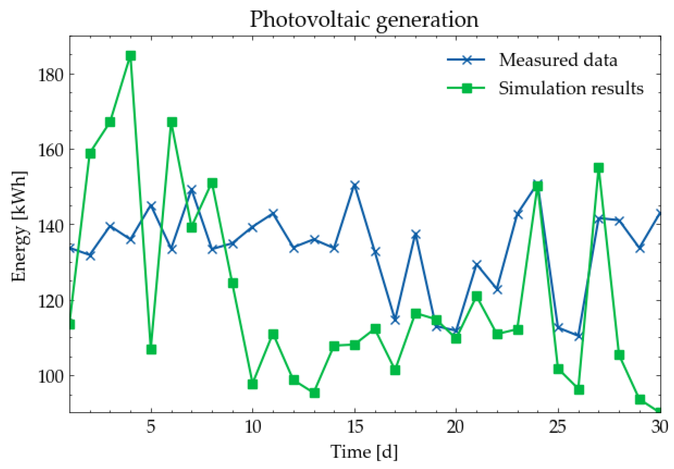
Figure 14, the results show a good match with the corresponding measurements on certain days. However, a deviation for the rest of the days is imported by the inconsistency between the used weather data and the actual conditions, as can be observed. The maximum deviation is 52.7 kWh on day 30, whereas the total estimation error in energy generation is 387 kWh (9.67%).
5. Scenarios Definition
5.1. Thermal Grid
Certain measures have been examined for the enhancement of system energy performance and are listed in
Table 9. The model has been simulated iteratively, changing certain design parameters and the solar fraction (f) value has been calculated and used as an evaluation index. A common simulation period has been selected to conduct the iterations, namely from 1 October until 8 October.
To evaluate solar contribution in terms of energy performance, the widely used index of solar fraction f is introduced, which is equivalent to the cumulative solar energy contribution to the total load demand over an entire period. Solar fraction f is defined as:
where
is the total generated solar energy over the entire period,
is the total energy demand over the entire period and
is the total biomass energy consumption over the entire period.
Measure #1 deals with the optimal temperature difference between collectors and TES for actuating circulating pumps. The current control system actuates the pumps of the secondary circuit when the temperature difference between the solar collector and the second tank exceeds the value of 7 °C (ΔΤ
on). Additionally, the pumps are turned off whenever this value becomes below 4 °C (ΔΤ
off). As stated by [
38], for optimal solar energy exploitation this value must be set in order to meet the constraint of the equation below.
where ε is the effectiveness of the solar field heat exchanger.
For the system under study, this leads to:
Thus, after solving the model iteratively, the optimal f value is found to be maximum for ΔΤon equal to 1.7 °C and ΔΤoff equal to 0.5 °C. It is assumed that the controller is sensitive to temperature differences of 0.5 °C and, thus, oscillations are avoided.
Measure #2 deals with the mass flow rates of the primary and secondary circuit pumps. These pumps are controlled with ON/OFF logic, so adjusting their amplitude is critical to system energy transactions. After an iterative process, the values obtained are 15,000 kg/h for the primary circuit pump and 6000 kg/h for the secondary circuit pump.
Measure #3 is related to the biomass boiler actuation condition. The boiler controller is based on ON/OFF logic and may lead to undesired oscillations, which result in increased biomass fuel consumption. The nominal setpoint values are 80 °C for turning on (low value) and 90 °C for turning off (high value). High values of these temperatures along with low increment between them, result in more frequent actuation of the boiler and therefore increase consumption. Based on the allowed operating conditions by the specifications of the installed radiators, supply and return temperatures can be set to 70 °C and 55 °C, respectively. This set of temperature values has been examined in this case. However, this measure cannot be considered reproducible, since radiator design temperatures are rarely adjustable.
Measure #4 includes the consideration of a smoother load profile over the day by decreasing the peak value and increasing load values over the rest of the day.
Measure #5 proposes the use of the existing load time series multiplied by a 90% factor, assuming that energy saving is achieved in the building complex. This measure implies the exploitation of passive building design interventions.
Measure #6 focuses on reducing the heat losses by increasing the insulation of the secondary circuit piping system. Existing piping system insulation material heat conductivity is 0.04 W/m∙K, while the solution of a material with a value of 0.035 W/m∙K is evaluated.
Measure #7 accounts for an increase in the TES system volume by 5 m3, reaching a total value of 54 m3.
Finally, a combination of all proposed measures is considered (Measure #8).
5.2. Electrical Grid
For the electrical grid, two measures have been selected and evaluated in comparison with the existing system (reference case). All of the cases under examination refer to the same time period of 15 days with a power load curve based on the data measured in June 2020 and already used for the validation in
Section 4.4.2 and the same initial condition of SoC (95%).
In the reference case, the PV installation of 51.5 kWp covers the power demand of the common spaces of a single building and an electric bicycle charging station. Since there is no backup power generator, if the battery DoD exceeds the maximum DoD (25%), a load-shedding option is actuated and the load is covered at 50% of the demand.
Measure #1 refers to the integration of the ORC system into the local energy system operation. As already mentioned, the 7 kWe of the ORC system is expected to be added to the power generation capacity of the PV system. The proposed control strategy for ORC is to inject power when battery daily DoD exceeds 25% and remains on until SoC exceeds the value of 80%.
Measure #2 deals with the possible benefits’ replacement of the current battery system with a Li-ion battery energy storage system of equivalent capacity. Since the battery cell model developed is specifically oriented for the Panasonic NMC 18650 cell, a battery pack with equivalent nominal capacity and voltage, and therefore energy capacity, needs to be considered, as reported in
Table 10. To satisfy this constraint, a 13s5670p configuration has been selected for the Li-ion battery pack examined for replacement. Additionally, based on the literature, the value of maximum DoD is set to 80% [
50], making this battery technology more appropriate for applications where deep cycling is performed. The voltage upper and lower thresholds of each cell are 4.2 V and 3.5 V, respectively.
6. Results and Discussion
6.1. Thermal Grid
The calculated values of f for each case under examination are listed in
Table 11, along with the total biomass energy consumption. Therefore, they represent two cumulative positive values over the entire period under examination.
Combining all of the proposed measures (Measure #8) leads to an increase in the f value from 12.64% to 37.26%. The largest effect is noticed by applying measure #3 (+28.70%), which is related to boiler temperature control. This is reasonable since keeping the water temperature at lower levels results in a lower enthalpy increase and therefore fuel consumption. Additionally, through Measure #5, where a smoother load profile is applied, a significant increase of 2.16% is achieved due to the load reduction and the consequent biomass consumption. Furthermore, as expected, increasing TES storage volume imports temporal flexibility to the system and leads to reduced energy consumption by the boiler. Lastly, Measure #1 has a positive effect on the f value, applying a control rule that ensures the minimization of heat losses.
6.2. Electrical Grid
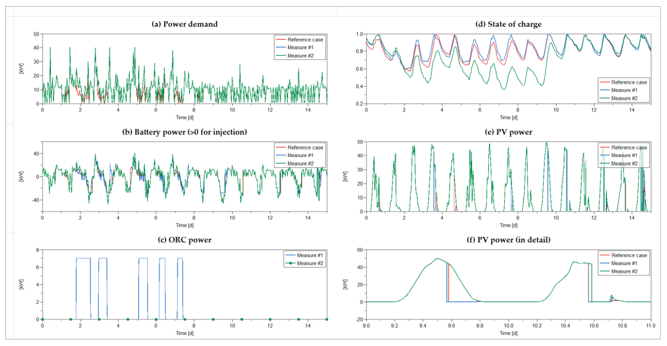
The corresponding results for each of the electrical grid measures under examination are presented in
Figure 15.
Figure 15a depicts that in the
reference case, the power demand is reduced in comparison with
Measures #1 and
#2 whenever the battery reaches its lower SoC limit, leading to load shedding. Lithium-ion battery, according to
Measure #2, operates within a larger SoC window as can be seen in
Figure 15d, which is also translated to higher values of battery income and outcome power in
Figure 15b. This results in a reduction in PV curtailment as well.
Figure 15e,f demonstrate that the PV power generation in the reference case and
Measure #1, is interrupted earlier than in
#2. This is due to control actions that secure that the condition of lead–acid battery maximum DoD is not violated.
Figure 15c shows the ORC power injected for
Measure #1 case, which explains the more narrow SoC operating range. It can also be observed that ORC is not delivering power to the load demand, since the Li-ion battery DoD does not exceed the maximum allowed value of 80%.
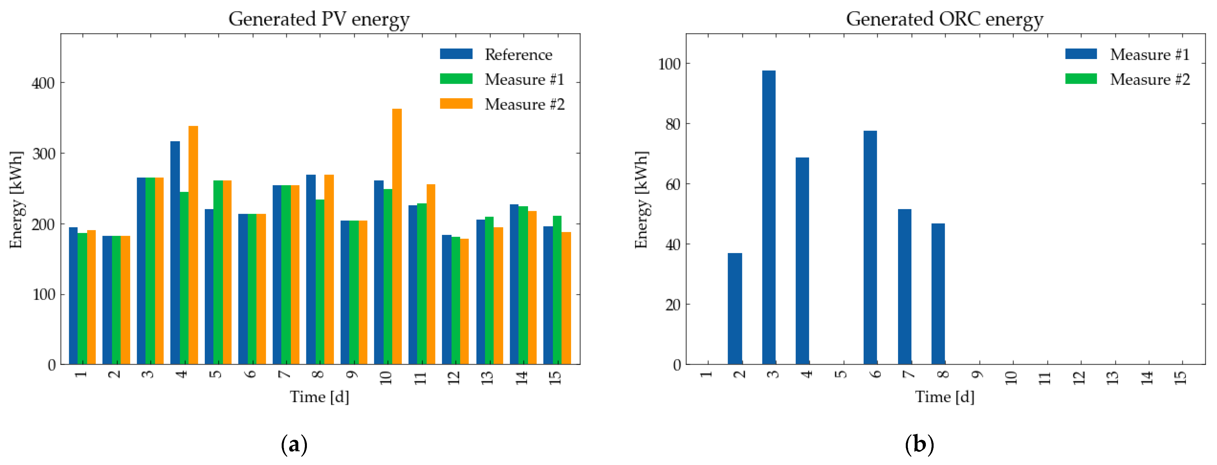
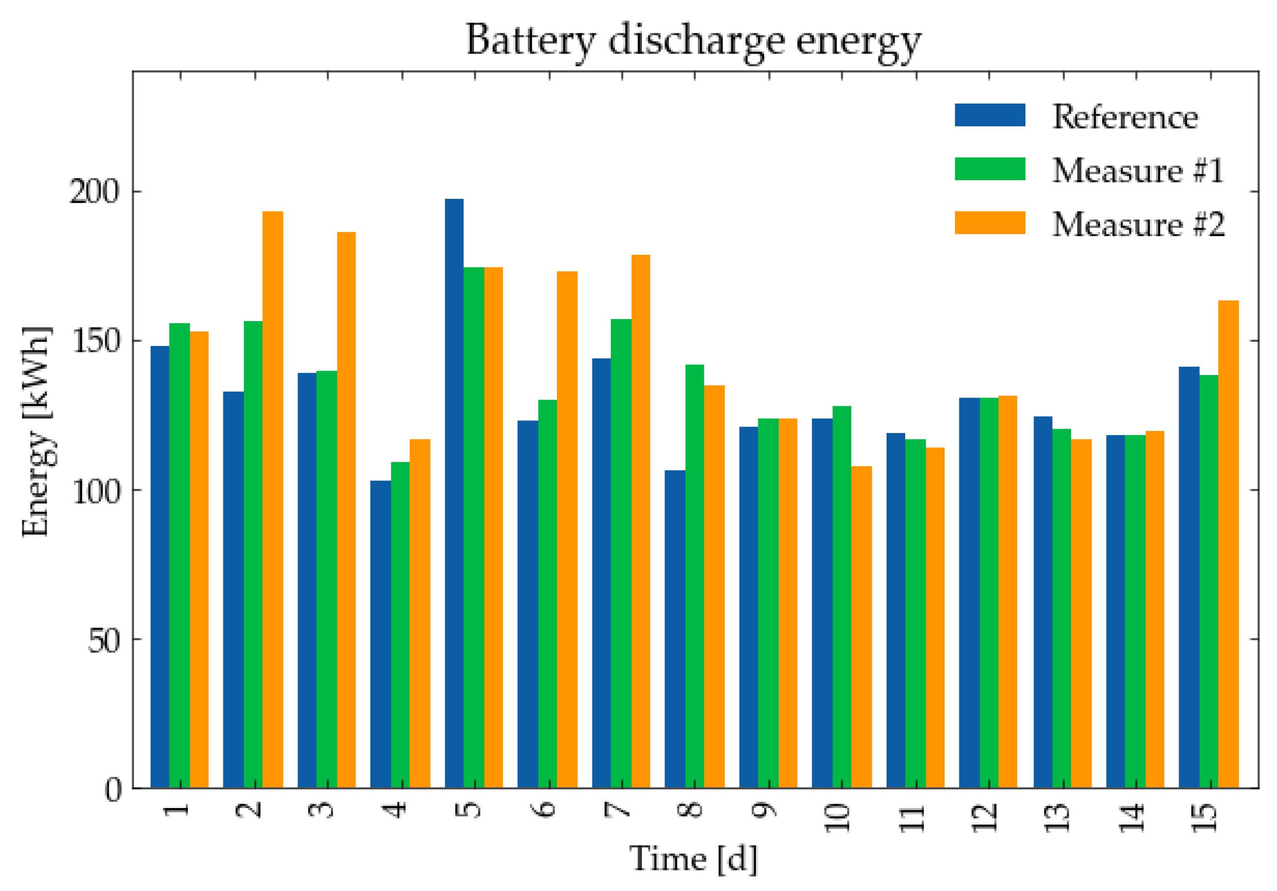
Figure 16 shows the daily evolution of the energy injected into the grid by (a) the ORC and (b) the PV systems. Regarding battery discharge energy, depicted in
Figure 17, a higher value is observed for
Measure #2 on almost all the days. This is strongly related to the fact that Li-ion batteries are preferred for deep-cycling applications. Additionally, as already mentioned above, since no PV curtailment takes place, the amount of energy generated by the PV is larger. ORC is only turned on in
Measure #1, since, as already mentioned, the Li-ion battery is able to cover the demand in the absence of PV generation. An interesting result is that on days 4, 8 and 10, more PV energy is produced in the
reference case than in
Measure #1. This is strongly related to the energy provided by the ORC system in
Measure #1 these days.
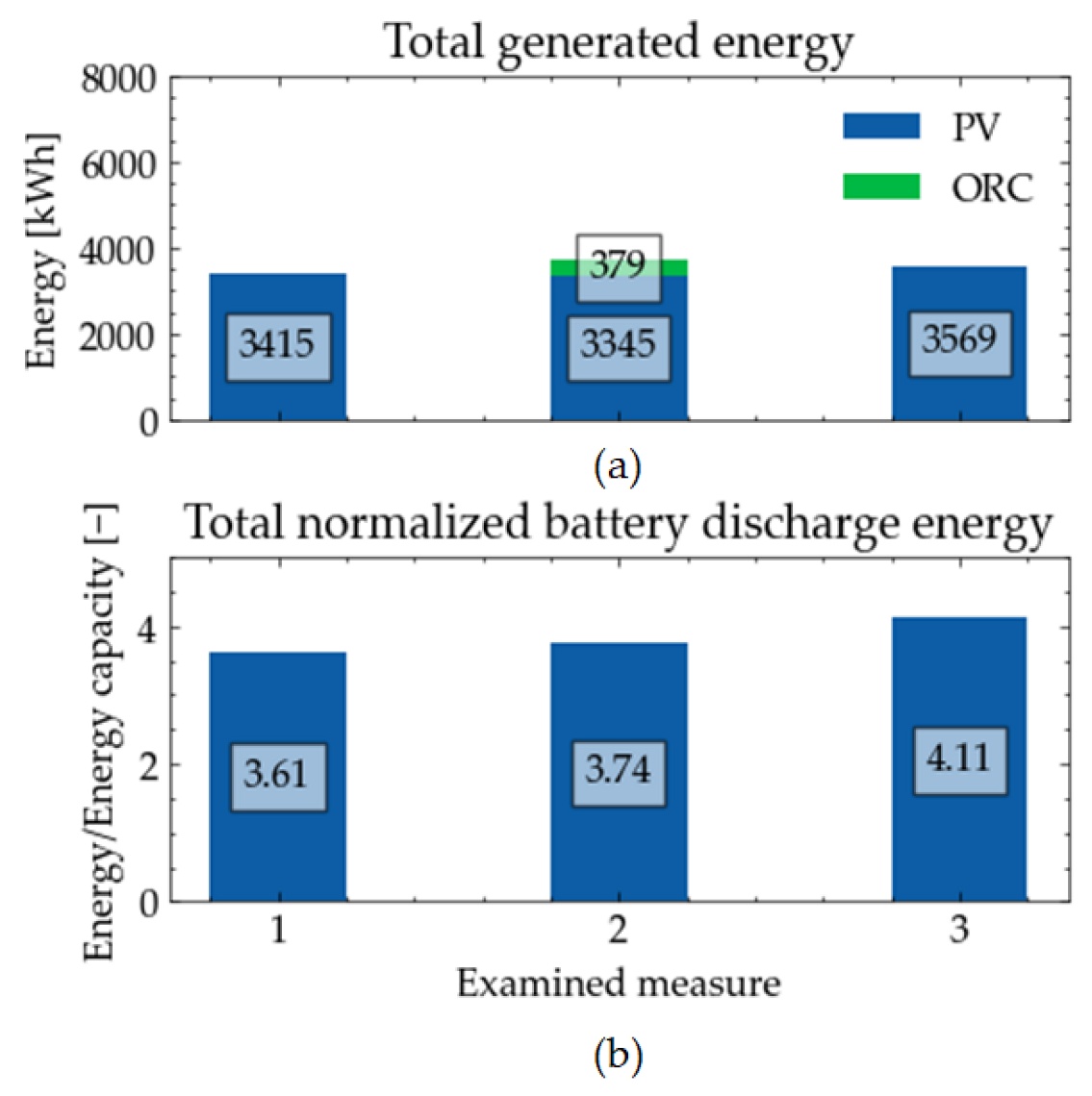
The amount of the total energy generated and the discharge energy injected by the battery are presented in
Figure 18a,b, respectively, for each measure examined. As mentioned in the results of daily energy production, even though in
Measure #1 PV energy is slightly less than in the reference case, the energy generated by the ORC increases the total renewable energy generation by 9.04%. Moreover, even though the total energy generated in
Measure #2 is increased by 4.53% in comparison with the reference case, it is lower than in
Measure #1. This can be explained by the microgrid energy management strategy considered, where ORC is only turned on when the battery SoC reaches its lower limit, acting as a backup generator. Therefore, the strategy does not focus on the maximization of ORC energy. Furthermore, the added ORC energy amount is not necessarily an advantage of
Measure #1 against
Measure #2, since biomass fuel consumption increases and must be taken into account.
7. Conclusions
A local energy system that incorporates solar thermal, biomass, PV, ORC and absorption refrigeration subsystems is examined in this study with the utilization of dynamic simulations. System representation is grounded on the mathematical modeling of each component.
State-of-the-art models have been exploited. Special focus has been given to the development of a single RC branch equivalent circuit model of an NMC Li-ion battery cell. The maximum sum squared error in the parameter estimation stage is limited to 359.6 mV. The model has been developed in Modelica language.
Validation of the thermal grid model has led to relative estimation errors of 4.4% for the solar generation and 5% for the total generation. Regarding the electrical grid, the relative estimation error of the PV generation is 9.67%.
The solar fraction f over a week in October has been studied under different scenarios defined by a proposed design and operating measures. Alternative measures showed great potential in f increase. Alteration in the biomass boiler operating temperature has led to a 16.06% rise in the value of f, whilst increasing thermal storage capacity and load smoothening led to a 1.57% and 2.16% rise, respectively. Applying a proposed control measure led to a 1.68% increase as well. Results showed that the combination of all measures led to a value of 37.26%.
The electrical grid operation over 15 days in June was also examined for different applied measures to study the effect of the installation of an ORC system (Measure #1) and a possible battery replacement (Measure #2). According to Measure #1, renewable energy generation was increased by 9.04% and for Measure #2 by 4.53%. However, ORC operation is not without constraints, since low solar fraction values lead to raised biomass fuel consumption. The Li-ion battery system examined as Measure #2 was found to be able to inject to the grid energy amounts of 4.11 times its energy capacity over the period under examination, while the corresponding value for the existing lead–acid battery system was lower (3.61). The larger contribution of the Li-ion battery system is mainly due to its larger value of maximum DoD.
These results are beneficial in multiple aspects. Practically, the application of the evaluated measures can lead to system performance enhancement with increased energy savings, energy efficiency and RES contribution. Additionally, economic benefits arise from the decrease in biomass fuel consumption. Furthermore, the efficient operation of the local electrical grid is a prerequisite for enabling financial schemes such as local energy communities (LECs). From a social perspective, results have shown that RES-based energy systems can support the supply of heating, cooling and electricity demand in public non-profit buildings, such as the student residences examined. From a technological point of view, the accurate computer-aided representation of an energy system with multiple cooperating energy vectors powered by RES enables two capabilities. First, to further examine alternative design and operation conditions for the current system. Moreover, to explore the utilization of the developed component models for the dynamic modeling of other energy systems.
Future work could draw on the developed models in order to enhance overall accuracy in system representation. The exploitation of measurements at different system points for the segmental validation of system components could lead to the retuning of model parameters in order to achieve enhanced accuracy. Moreover, the input of accurate weather data can strengthen the validation process. On top of that, the option of energy management strategies based on sophisticated control techniques for real-time simulations will be enabled, which will further lead to optimized system performance.
Author Contributions
Conceptualization, R.R. and P.I.; methodology, R.R. and P.I.; software, R.R.; validation, R.R.; investigation, R.R. and P.I.; writing—original draft preparation, R.R., P.I., N.N., A.T. and E.K.; writing—review and editing, R.R., P.I., N.N., A.T. and E.K.; supervision, N.N., A.T. and E.K. All authors have read and agreed to the published version of the manuscript.
Funding
This work has been carried out in the framework of the European Union’s Horizon 2020 research and innovation programme under grant agreement No 824342 (RENewAble Integration and SuStainAbility iN energy CommunitiEs-RENAISSANCE).
Institutional Review Board Statement
Not applicable.
Data Availability Statement
Not applicable.
Conflicts of Interest
The authors declare no conflict of interest.
Nomenclature
| COP | Coefficient of Performance |
| CCHP | Combined Cooling, Heat and Power |
| CHP | Combined Heat and Power |
| DERs | Distributed Energy Resources |
| DHW | Domestic Hot Water |
| DoD | Depth of Discharge |
| ECM | Equivalent Circuit Model |
| GWP | Global Warming Potential |
| LECs | Local Energy Communities |
| MPPT | Maximum Power Point Tracker |
| OCV | Open-circuit Voltage |
| ODP | Ozone Depletion Potential |
| OPzS | Ortsfest (stationary) PanZerplatte (tubular plate) Flüssig (flooded) |
| ORC | Organic Rankine Cycle |
| PLR | Part-load Ratio |
| RES | Renewable Energy Sources |
| SoC | State of Charge |
| TES | Thermal Energy Storage |
References
- Kalair, A.; Abas, N.; Saleem, M.S.; Kalair, A.R.; Khan, N. Role of Energy Storage Systems in Energy Transition from Fossil Fuels to Renewables. Energy Storage 2021, 3, e135. [Google Scholar] [CrossRef] [Green Version]
- López González, D.M.; Garcia Rendon, J. Opportunities and Challenges of Mainstreaming Distributed Energy Resources towards the Transition to More Efficient and Resilient Energy Markets. Renew. Sustain. Energy Rev. 2022, 157, 112018. [Google Scholar] [CrossRef]
- Subramanian, A.; Gundersen, T.; Adams, T. Modeling and Simulation of Energy Systems: A Review. Processes 2018, 6, 238. [Google Scholar] [CrossRef] [Green Version]
- Battula, A.R.; Vuddanti, S.; Salkuti, S.R. Review of Energy Management System Approaches in Microgrids. Energies 2021, 14, 5459. [Google Scholar] [CrossRef]
- Palomba, V.; Borri, E.; Charalampidis, A.; Frazzica, A.; Cabeza, L.F.; Karellas, S. Implementation of a Solar-Biomass System for Multi-Family Houses: Towards 100% Renewable Energy Utilization. Renew. Energy 2020, 166, 190–209. [Google Scholar] [CrossRef]
- Zisopoulos, G.; Nesiadis, A.; Atsonios, K.; Nikolopoulos, N.; Stitou, D.; Coca-Ortegón, A. Conceptual Design and Dynamic Simulation of an Integrated Solar Driven Thermal System with Thermochemical Energy Storage for Heating and Cooling. J. Energy Storage 2021, 41, 102870. [Google Scholar] [CrossRef]
- Abusaibaa, G.Y.; Al-Aasam, A.B.; Al-Waeli, A.H.A.; Al-Fatlawi, A.W.A.; Sopian, K.B. Performance Analysis of Solar Absorption Cooling Systems in Iraq. Int. J. Renew. Energy Res. 2020, 10, 223–230. [Google Scholar]
- Orosz, M.; Dickes, R. Solar Thermal Powered Organic Rankine Cycles. In Organic Rankine Cycle (ORC) Power Systems; Elsevier: Amsterdam, The Netherlands, 2017; pp. 569–612. ISBN 978-0-08-100510-1. [Google Scholar]
- Fatigati, F.; Vittorini, D.; Wang, Y.; Song, J.; Markides, C.N.; Cipollone, R. Design and Operational Control Strategy for Optimum Off-Design Performance of an ORC Plant for Low-Grade Waste Heat Recovery. Energies 2020, 13, 5846. [Google Scholar] [CrossRef]
- Fitri, S.P.; Zaman, M.B.; Azizi, F.A. Design of Organic Rankine Cycle (ORC) Power Plant Systems by Using Flat-Plate Solar Collector. IJMEIR 2019, 4, 199–207. [Google Scholar] [CrossRef]
- Casella, F.; Mathijssen, T.; Colonna, P.; van Buijtenen, J. Dynamic Modeling of Organic Rankine Cycle Power Systems. J. Eng. Gas Turbines Power 2013, 135, 042310. [Google Scholar] [CrossRef]
- Twomey, B. Dynamic Simulation and Experimental Validation of an Organic Rankine Cycle Model. Ph.D. Thesis, The University of Queensland, Brisbane, Australia, 2016. [Google Scholar]
- Dabwan, Y.N.; Pei, G. A Novel Integrated Solar Gas Turbine Trigeneration System for Production of Power, Heat and Cooling: Thermodynamic-Economic-Environmental Analysis. Renew. Energy 2020, 152, 925–941. [Google Scholar] [CrossRef]
- Jalalizadeh, M.; Fayaz, R.; Delfani, S.; Mosleh, H.J.; Karami, M. Dynamic Simulation of a Trigeneration System Using an Absorption Cooling System and Building Integrated Photovoltaic Thermal Solar Collectors. J. Build. Eng. 2021, 43, 102482. [Google Scholar] [CrossRef]
- Calise, F.; Dentice d’Accadia, M.; Palombo, A.; Vanoli, L. Dynamic Simulation of a Novel High-Temperature Solar Trigeneration System Based on Concentrating Photovoltaic/Thermal Collectors. Energy 2013, 61, 72–86. [Google Scholar] [CrossRef]
- Acevedo, L.; Uche, J.; Del Almo, A.; Círez, F.; Usón, S.; Martínez, A.; Guedea, I. Dynamic Simulation of a Trigeneration Scheme for Domestic Purposes Based on Hybrid Techniques. Energies 2016, 9, 1013. [Google Scholar] [CrossRef] [Green Version]
- Doracic, B.; Grozdek, M.; Puksec, T.; Duic, N. Excess Heat Utilization Combined with Thermal Storage Integration in District Heating Systems Using Renewables. Therm. Sci. 2020, 24, 3673–3684. [Google Scholar] [CrossRef]
- Hirmiz, R.; Lightstone, M.F.; Cotton, J.S. Performance Enhancement of Solar Absorption Cooling Systems Using Thermal Energy Storage with Phase Change Materials. Appl. Energy 2018, 223, 11–29. [Google Scholar] [CrossRef]
- Velut, S.; Andreasson, J.; Navratil, J.; Åberg, M. A Modelica-Based Solution for the Simulation and Optimization of Microgrids Proceedings of the Asian Modelica Conference; Linköping University Electronic Press: Linköping, Sweden, 2020; pp. 41–47. [Google Scholar]
- MacRae, N.; Batteh, J.; Velut, S.; Skrivan, W.; Khan, I.; Jang, D. Micro-Grid Design and Cost Optimization Using Modelica. In Proceedings of the American Modelica Conference 2020, Boulder, CO, USA, 23–25 March 2020; Linköping University Electronic Press: Boulder, CO, USA, 2020; pp. 18–27. [Google Scholar] [CrossRef]
- Al-Nimr, M.A.; Al-Ammari, W.A. A Novel PVT/PTC/ORC Solar Power System with PV Totally Immersed in Transparent Organic Fluid. Int. J. Energy Res. 2019, 43, 4766–4782. [Google Scholar] [CrossRef]
- Ungureşan, P.; Petreuş, D.; Pocola, A.; Bălan, M. Potential of Solar ORC and PV Systems to Provide Electricity under Romanian Climatic Conditions. Energy Procedia 2016, 85, 584–593. [Google Scholar] [CrossRef] [Green Version]
- Tourkov, K.; Schaefer, L. Performance Evaluation of a PVT/ORC (Photovoltaic Thermal/Organic Rankine Cycle) System with Optimization of the ORC and Evaluation of Several PV (Photovoltaic) Materials. Energy 2015, 82, 839–849. [Google Scholar] [CrossRef]
- Sarita, K.; Devarapalli, R.; Rai, P. Modeling and Control of Dynamic Battery Storage System Used in Hybrid Grid. Energy Storage 2020, 2, e146. [Google Scholar] [CrossRef] [Green Version]
- Jufri, F.H.; Aryani, D.R.; Garniwa, I.; Sudiarto, B. Optimal Battery Energy Storage Dispatch Strategy for Small-Scale Isolated Hybrid Renewable Energy System with Different Load Profile Patterns. Energies 2021, 14, 3139. [Google Scholar] [CrossRef]
- Chen, M.; Rincon-Mora, G.A. Accurate Electrical Battery Model Capable of Predicting Runtime and I-V Performance. IEEE Trans. Energy Convers. 2006, 21, 504–511. [Google Scholar] [CrossRef]
- Tamilselvi, S.; Gunasundari, S.; Karuppiah, N.; Razak RK, A.; Madhusudan, S.; Nagarajan, V.M.; Sathish, T.; Shamim, M.Z.M.; Saleel, C.A.; Afzal, A. A Review on Battery Modelling Techniques. Sustainability 2021, 13, 10042. [Google Scholar] [CrossRef]
- Kebede, A.A.; Coosemans, T.; Messagie, M.; Jemal, T.; Behabtu, H.A.; Van Mierlo, J.; Berecibar, M. Techno-Economic Analysis of Lithium-Ion and Lead-Acid Batteries in Stationary Energy Storage Application. J. Energy Storage 2021, 40, 102748. [Google Scholar] [CrossRef]
- Paul Ayeng’o, S.; Schirmer, T.; Kairies, K.-P.; Axelsen, H.; Uwe Sauer, D. Comparison of Off-Grid Power Supply Systems Using Lead-Acid and Lithium-Ion Batteries. Sol. Energy 2018, 162, 140–152. [Google Scholar] [CrossRef]
- Ayuso, P.; Beltran, H.; Segarra-Tamarit, J.; Pérez, E. Optimized Profitability of LFP and NMC Li-Ion Batteries in Residential PV Applications. Math. Comput. Simul. 2021, 183, 97–115. [Google Scholar] [CrossRef]
- Marshall, P.G.; Wongpanyo, W.; Sittisun, P.; Rakwichian, W.; Thanarak, P.; Vichanpol, B. Comparison of Energy Storage Technologies for a Notional, Isolated Community Microgrid. J. Renew. Energy Smart Grid Technol. 2020, 15, 14. [Google Scholar]
- Beltran, H.; Ayuso, P.; Pérez, E. Lifetime Expectancy of Li-Ion Batteries Used for Residential Solar Storage. Energies 2020, 13, 568. [Google Scholar] [CrossRef] [Green Version]
- Botsaris, P.N.; Lymperopoulos, K.; Pechtelidis, A. Preliminary Evaluation of Operational Results of RES Systems Integrated in Students’ Residences in Xanthi, Greece. IOP Conf. Ser. Earth Environ. Sci. 2020, 410, 012048. [Google Scholar] [CrossRef]
- Papatsounis, A.G.; Botsaris, P.N.; Lymperopoulos, K.A.; Rotas, R.; Kanellia, Z.; Iliadis, P.; Nikolopoulos, N. Operation Assessment of a Hybrid Solar-Biomass Energy System with Absorption Refrigeration Scenarios. Energy Sources Part A Recovery Util. Environ. Eff. 2022, 44, 700–717. [Google Scholar] [CrossRef]
- Botsaris, P.N.; Lymperopoulos, K.A.; Giourka, P.; Bekakos, P.; Pistofidis, P.; Pecthelidis, A. Integration of Renewable Energy Technologies in Student Residences of Xanthi and Results of Project REUNI; Solar Energy Institute: Thessaloniki, Greece, 2018. [Google Scholar]
- Brkic, J.; Ceran, M.; Elmoghazy, M.; Kavlak, R.; Haumer, A.; Kral, C. Open Source PhotoVoltaics Library for Systemic Investigations. In Proceedings of the 13th International Modelica Conference, Regensburg, Germany, 4–6 March 2019; pp. 41–50. [Google Scholar]
- Pfeifroth, U.; Kothe, S.; Trentmann, J.; Hollmann, R.; Fuchs, P.; Kaiser, J.; Werscheck, M. Surface Radiation Data Set—Heliosat (SARAH)—Edition 2.1, Satellite Application Facility on Climate Monitoring. 2019. Available online: https://wui.cmsaf.eu/safira/action/viewDoiDetails?acronym=SARAH_V002_01 (accessed on 15 May 2022).
- Duffie (Deceased), J.A.; Beckman, W.A.; Blair, N. Solar Engineering of Thermal Processes, Photovoltaics and Wind, 1st ed.; Wiley: Hoboken, NJ, USA, 2020; ISBN 978-1-119-54028-1. [Google Scholar]
- Regulation (EU) No 517/2014 of the European Parliament and of the Council of 16 April 2014 on Fluorinated Greenhouse Gases and Repealing Regulation (EC) No 842/2006Text with EEA Relevance. Available online: https://eur-lex.europa.eu/legal-content/EN/TXT/PDF/?uri=CELEX:32014R0517&from=EN (accessed on 1 January 2022).
- Quoilin, S.; Desideri, A.; Wronski, J.; Bell, I.; Lemort, V. ThermoCycle: A Modelica Library for the Simulation of Thermodynamic Systems. In Proceedings of the 10th International Modelica Conference, Lund, Sweden, 10–12 March 2014; Linköping University Electronic Press: Lund, Sweden, 2014; pp. 683–692. [Google Scholar]
- Casella, F.; Richter, C. ExternalMedia: A Library for Easy Re-Use of External Fluid Property Code in Modelica. In Proceedings of the 6th International Modelica Conference, Bielefeld, Germany, 3 March 2008; pp. 157–161. [Google Scholar]
- Bell, I.H.; Wronski, J.; Quoilin, S.; Lemort, V. Pure and Pseudo-Pure Fluid Thermophysical Property Evaluation and the Open-Source Thermophysical Property Library CoolProp. Ind. Eng. Chem. Res. 2014, 53, 2498–2508. [Google Scholar] [CrossRef] [PubMed] [Green Version]
- Lemmon, E.W.; Bell, I.H.; Huber, M.L.; McLinden, M.O. NIST Standard Reference Database 23: Reference Fluid Thermodynamic and Transport Properties-REFPROP, Version 10.0; National Institute of Standards and Technology: Gaithersburg, MD, USA, 2018. [Google Scholar]
- Plett, G.L. Battery Management Systems, Volume 2: Equivalent-Circuit Methods; Artech House Power Engineering and Power Electronics; Artech House: Boston, MA, USA, 2016; ISBN 978-1-63081-027-6. [Google Scholar]
- Jantharamin, N.; Zhang, L. A New Dynamic Model for Lead-Acid Batteries. In Proceedings of the 4th IET International Conference on Power Electronics, Machines and Drives (PEMD 2008), York, UK, 2–4 April 2008; IEE: York, UK, 2008; pp. 86–90. [Google Scholar]
- Ceraolo, M. New Dynamical Models of Lead-Acid Batteries. IEEE Trans. Power Syst. 2000, 15, 1184–1190. [Google Scholar] [CrossRef] [Green Version]
- Huria, T.; Ceraolo, M.; Gazzarri, J.; Jackey, R. High Fidelity Electrical Model with Thermal Dependence for Characterization and Simulation of High Power Lithium Battery Cells. In Proceedings of the 2012 IEEE International Electric Vehicle Conference, Greenville, SC, USA, 4–8 March 2012; IEEE: Greenville, SC, USA, 2012; pp. 1–8. [Google Scholar]
- Zheng, F.; Xing, Y.; Jiang, J.; Sun, B.; Kim, J.; Pecht, M. Influence of Different Open Circuit Voltage Tests on State of Charge Online Estimation for Lithium-Ion Batteries. Appl. Energy 2016, 183, 513–525. [Google Scholar] [CrossRef]
- Dorf, E.R.C. Electrical Engineering Handbook; CRC Press LLC: Boca Raton, FL, USA, 2000; ISBN 978-0-8493-1586-2. [Google Scholar]
- Podder, S.; Khan, M.Z.R. Comparison of Lead Acid and Li-Ion Battery in Solar Home System of Bangladesh. In Proceedings of the 2016 5th International Conference on Informatics, Electronics and Vision (ICIEV), Piscataway, NJ, USA, 13–14 May 2016; pp. 434–438. [Google Scholar]
Figure 1.
Model development and evaluation methodology that has been followed.
Figure 1.
Model development and evaluation methodology that has been followed.
Figure 2.
Presentation of the local energy system under study.
Figure 2.
Presentation of the local energy system under study.
Figure 3.
Energy management overview of the electrical grid.
Figure 3.
Energy management overview of the electrical grid.
Figure 4.
Verification of the ORC model developed in Dymola (below) against the ASPEN Plus Dynamics model (above).
Figure 4.
Verification of the ORC model developed in Dymola (below) against the ASPEN Plus Dynamics model (above).
Figure 5.
Equivalent circuit topology of the model used for lead–acid battery cell.
Figure 5.
Equivalent circuit topology of the model used for lead–acid battery cell.
Figure 6.
One-dimensional look-up tables for OPzS battery cell equivalent circuit: (a) Self-discharge resistance Rsd, (b) polarization capacitance Cov and (c) polarization resistance Rbdi.
Figure 6.
One-dimensional look-up tables for OPzS battery cell equivalent circuit: (a) Self-discharge resistance Rsd, (b) polarization capacitance Cov and (c) polarization resistance Rbdi.
Figure 7.
The equivalent circuit model with a single RC branch used for this study.
Figure 7.
The equivalent circuit model with a single RC branch used for this study.
Figure 8.
Battery cell model with 1 RC branch and thermal dependence.
Figure 8.
Battery cell model with 1 RC branch and thermal dependence.
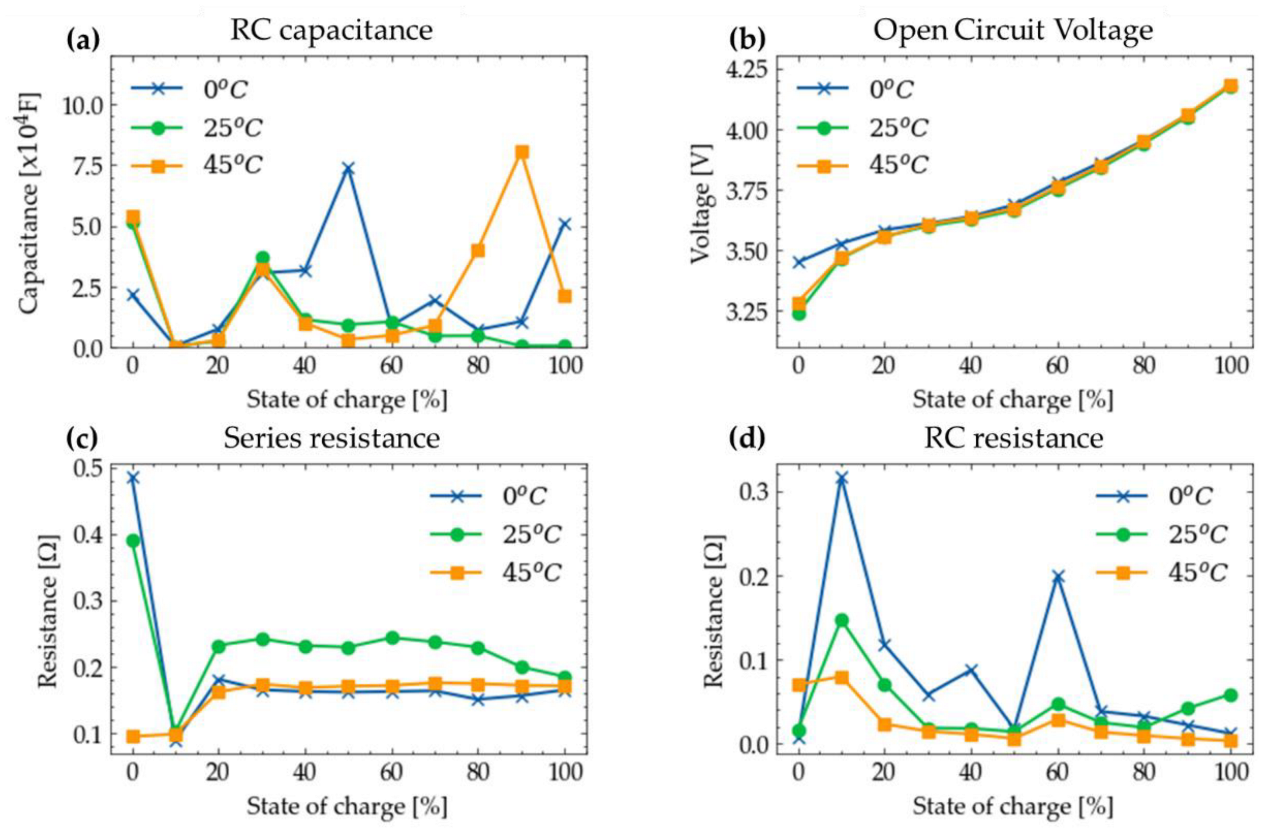
Figure 9.
Two-dimensional look-up tables of Li-ion cell ECM parameters for a single number of RC branches, namely (a) RC capacitance, (b) open circuit voltage, (c) series resistance and (d) RC resistance.
Figure 9.
Two-dimensional look-up tables of Li-ion cell ECM parameters for a single number of RC branches, namely (a) RC capacitance, (b) open circuit voltage, (c) series resistance and (d) RC resistance.
Figure 10.
Local thermal grid model.
Figure 10.
Local thermal grid model.
Figure 11.
Local electrical grid model connected with the ORC system, powered by solar thermal energy and biomass.
Figure 11.
Local electrical grid model connected with the ORC system, powered by solar thermal energy and biomass.
Figure 12.
Thermal grid validation against solar energy generation measurements.
Figure 12.
Thermal grid validation against solar energy generation measurements.
Figure 13.
Thermal grid validation. Simulation results against total energy generation measurements.
Figure 13.
Thermal grid validation. Simulation results against total energy generation measurements.
Figure 14.
Electrical grid validation. Simulation results against PV generation measurements.
Figure 14.
Electrical grid validation. Simulation results against PV generation measurements.
Figure 15.
Power balance and state of charge (SoC) evolution during the period examined. (a) Power demand, (b) injected battery power, (c) ORC power, (d) battery SoC, (e) PV power and (f) PV power between days 9 and 11 in detail.
Figure 15.
Power balance and state of charge (SoC) evolution during the period examined. (a) Power demand, (b) injected battery power, (c) ORC power, (d) battery SoC, (e) PV power and (f) PV power between days 9 and 11 in detail.
Figure 16.
Daily energy amounts injected for each proposed measure by (a) PV and (b) ORC systems.
Figure 16.
Daily energy amounts injected for each proposed measure by (a) PV and (b) ORC systems.
Figure 17.
Daily energy amount injected for each proposed measure by the battery system.
Figure 17.
Daily energy amount injected for each proposed measure by the battery system.
Figure 18.
Total energy injected for each proposed measure by (a) RES and (b) battery system normalized to nominal discharge energy capacity.
Figure 18.
Total energy injected for each proposed measure by (a) RES and (b) battery system normalized to nominal discharge energy capacity.
Table 1.
Main parameter values of the thermal grid.
Table 1.
Main parameter values of the thermal grid.
| Asset | Parameter | Value |
|---|
| Solar thermal field | Number of collector modules | 720 |
| Type of collector | Flat plate |
| Gross area per module | 2.58 m2 |
| Total gross area | 1857.6 m2 |
| Surface tilt angle | 45° |
| Biomass boiler | Nominal thermal power capacity | 1.15 MWth |
| Fuel | Pellet |
| Nominal efficiency | 0.87 |
| Buffer tank volume | 4.2 m3 |
| Total mass | 5000 kg |
| Absorption chiller | Type | Single-effect hot water-fired |
| Cooling power capacity | 316 kWc |
| Nominal COP | 0.78 |
| Cooling tower | Power capacity | 720.5 kW |
| ORC system | Nominal power output | 7 kWe |
| Nominal thermal power input | 102 kW |
| Hot water tanks | Number of tanks | 4 |
| Total capacity | 49 m3 |
| Insulation thickness | 0.05 m |
Table 2.
Main parameter values of the electrical grid.
Table 2.
Main parameter values of the electrical grid.
| Asset | Parameter | Value |
|---|
| Photovoltaic system | Panel type | Polycrystalline |
| PV nominal power capacity | 51.5 kWp |
| Number of panels | 198 |
| Battery system | Battery cell type | Lead–acid |
| Battery system nominal energy capacity | 544.3 kWh |
| Battery system configuration | 24s3p |
| Battery system nominal voltage | 48 V |
| Battery system nominal capacity | 11,340 Ah |
| Maximum daily allowable Depth of discharge (DoD) | 25% |
Table 3.
Organic Rankine Cycle: Manufacturer’s specifications.
Table 3.
Organic Rankine Cycle: Manufacturer’s specifications.
| Technical Specification | Value |
|---|
| Working fluid | R245fa |
| Nominal power output | 7 kWe |
| Nominal condenser water inlet/outlet temperature | 30/37 °C |
| Nominal evaporator water inlet/outlet temperature | 90/75 °C |
| Expander type | Single-screw |
| Displacement volume | 47 m3/h |
| Expansion ratio | 2.5 |
Table 4.
Organic Rankine Cycle: Thermodynamic states used for the model.
Table 4.
Organic Rankine Cycle: Thermodynamic states used for the model.
| Thermodynamic State | Quantity |
|---|
| Pressure [bar] | Temperature [°C] | Phase |
|---|
| 1 | 3.05 | 35 | Subcooled liquid |
| 2 | 7.773 | 35.6 | Subcooled liquid |
| 3 | 7.7 | 84 | Superheated vapor |
| 4 | 3.103 | 62.3 | Superheated vapor |
Table 5.
Thermodynamic states of the Organic Rankine Cycle (ORC) under examination.
Table 5.
Thermodynamic states of the Organic Rankine Cycle (ORC) under examination.
| Thermodynamic State | Quantity |
|---|
| Pressure [bar] | Temperature [°C] |
|---|
| 1 | 7 | 33 |
| 2 | 20 | 35.6 |
| 3 | 20 | 77.5 |
| 4 | 10.5 | 52.2 |
Table 6.
Absorption chiller technical specifications.
Table 6.
Absorption chiller technical specifications.
| Parameter | Value |
|---|
| Cooling capacity | 316 kWc |
| Nominal COP | 0.78 |
| Condenser nominal inlet temperature | 29 °C |
| Condenser nominal outlet temperature | 36 °C |
| Evaporator nominal inlet temperature | 12 °C |
| Evaporator nominal outlet temperature | 7 °C |
| Generator nominal inlet temperature | 90 °C |
| Generator nominal outlet temperature | 80 °C |
| Hot water mass flow rate | 10.1 kg/s |
| Chilled water mass flow rate | 15.1 kg/s |
| Cooling water mass flow rate | 25 kg/s |
Table 7.
Battery cell capacity dependency on temperature for discharge and charge processes.
Table 7.
Battery cell capacity dependency on temperature for discharge and charge processes.
| Discharge |
| Temperature | −10 °C | 0 °C | 25 °C | 60 °C |
| Relative capacity | 75% | 80% | 100% | 100% |
| Charge |
| Temperature | 0 °C | 5 °C | 25 °C | 45 °C |
| Relative capacity | 80% | 90% | 100% | 95% |
Table 8.
Li-ion battery parameter estimation results. Sum squared error for measurements conducted in three different temperatures.
Table 8.
Li-ion battery parameter estimation results. Sum squared error for measurements conducted in three different temperatures.
| Temperature | Sum Squared Error (mV) |
|---|
| 0 °C | 125.2 |
| 25 °C | 359.6 |
| 45 °C | 45.2 |
Table 9.
Comparison of proposed measures based on simulation results.
Table 9.
Comparison of proposed measures based on simulation results.
| Measure | System Point | Action |
|---|
| Reference case | Default design condition | None |
| #1 | Secondary pump control system | Change actuation condition |
| #2 | Primary and secondary pumps | Change mass flow rates |
| #3 | Biomass boiler | Change limits in hysteresis control (Ton/Toff) |
| #4 | Load demand | Decrease peak value (smoother load) |
| #5 | Load demand | Decrease total load by 10% (passive measures) |
| #6 | Piping system | Decrease heat losses (insulation) |
| #7 | Hot water tanks | Increase storage volume |
| #8 | Overall system | Combination of all |
Table 10.
Current and proposed battery system specifications.
Table 10.
Current and proposed battery system specifications.
| Battery System | Current | Proposed |
|---|
| Cell chemistry/technology | OPzS lead–acid | NMC lithium-ion |
| Cell nominal capacity | 3780 Ah | 2 Ah |
| Cell nominal voltage | 2 V | 3.6 V |
| Battery pack configuration | 24s3p | 13s5670p |
| Battery pack nominal capacity | 11,340 Ah | 11,340 Ah |
| Battery pack nominal voltage | 48 V | 46.8 V |
| Battery pack nominal energy capacity | 544.3 kWh | 530.7 kWh |
| Maximum daily DoD | 25% (manufacturer) | 80% |
| Maximum cut-off voltage per cell | 3.85 V | 3.5 V |
| Minimum cut-off voltage per cell | 4.1 V | 4.2 V |
Table 11.
Solar fraction (f) and biomass energy consumption values for each case under examination.
Table 11.
Solar fraction (f) and biomass energy consumption values for each case under examination.
| Case Examined | Solar
Fraction | Solar Fraction Increase | Biomass Energy Consumption (MWh) | Reduction in Biomass Energy Consumption (%) |
|---|
| Existing system | 12.64% | - | 70.1 | - |
| Measure #1 | 14.32% | 1.68% | 68.8 | 1.85% |
| Measure #2 | 12.93% | 0.29% | 69.9 | 0.29% |
| Measure #3 | 28.70% | 16.06% | 57.2 | 18.40% |
| Measure #4 | 13.62% | 0.98% | 68.9 | 1.71% |
| Measure #5 | 14.80% | 2.16% | 51.3 | 26.82% |
| Measure #6 | 12.81% | 0.17% | 69.9 | 0.29% |
| Measure #7 | 14.21% | 1.57% | 68.8 | 1.85% |
| Measure #8 | 37.26% | 24.62% | 43.8 | 37.52% |
| Publisher’s Note: MDPI stays neutral with regard to jurisdictional claims in published maps and institutional affiliations. |
© 2022 by the authors. Licensee MDPI, Basel, Switzerland. This article is an open access article distributed under the terms and conditions of the Creative Commons Attribution (CC BY) license (https://creativecommons.org/licenses/by/4.0/).

 ,
, 


