Abstract
The paper investigated the problem of selecting/finding the optimal process conditions for gas condensate wells. The well process conditions imply a set of parameters that characterize its operation. The optimization of process conditions provides for the efficient operation of an oil and gas field while meeting the defined boundary and initial conditions, and allows for the process/production goal to be achieved. This paper proposed using the tree-structured Parzen estimator (TPE), which allows for the results from previous iterations to be considered, in order to identify the most promising region of conditions, thereby increasing the optimization efficiency. The movement of multiphase fluid inside the pipeline system (also in the borehole) must be calculated to solve the process optimization problem. The optimization module was integrated into the hydraulic and unsteady state multiphase flow calculations inside the well and the pipeline. The platform created allows for the process conditions at gas condensate fields to be identified via the use of numerical methods. The proposed optimization algorithm was tested in delivering the task of optimizing the process conditions in 13 producing wells in a part of a real gas condensate field in Western Siberia. The engineering problem of optimizing the production of gas and the gas condensate was solved as a consequence of the calculations performed.
1. Introduction
Finding an optimal solution for almost any process is a challenging mathematical problem, generally solvable with the aid of optimization algorithms, which must be selected based on the problem type, initial, and boundary conditions. Traditionally, the random search and grid search algorithms are used for optimization. The efficient operation of oil and gas fields is largely determined by the hydrocarbon production process conditions, which may ensure the long-life of wells while maintaining a high recovery factor. The steady-state process conditions of a well are understood as a set of its operating parameters that ensure the oil, gas, and gas condensate yield for a certain time interval.
The main process variables of a well will differ for various fields, subject to the condition of hydrocarbons in the formation. Thus, purely for oil fields, the main variables are the bottom hole pressure and liquid column level in the hole, with the control tool represented by the pump operating mode in the case of artificially lifted oil. For gas and gas condensate fields, primary production is used, with the well head pressure being the main parameter and the nominal bore of the surface choke will be the tool to control the well performance. When it changes, the well process conditions change. The duration for a well transition to a steady-state operation varies and depends on the formation deliverability and formation-pressure conductivity, formation pressure, fluid composition, and on the relative change in the rate. The steady-state operation of wells is characterized by a constant rate and the readings of pressure gauges connected to the tubing and the inner annulus.
The movement of gas and liquid streams inside the well can be simulated using a system of continuity equations, conserving the impulse for the gas and liquid phases [1,2,3,4,5,6], and the equation for the total enthalpy of the mixture in the assigned volume and for the weight of a separate component considering friction, specific enthalpy, and heat exchange (gas/liquid, wall/gas, liquid/gas, wall/liquid). The system of equations cannot be solved analytically in the general case, so numerical methods will be applied in the calculation.
The optimization module for the well process conditions is integrated into the hydraulic calculation [7,8,9]. The optimization result is the selected nominal bores of the surface choke of known producing wells, which ensures the minimum value of the target function. In practice, due to the vast number of variables, the problem of optimizing the well process conditions has a large scale. To solve this, we used the Bayesian optimization algorithm, which considers the data of previous iterations to identify the most promising parameter region.
The proposed algorithms promote the development of the theoretical aspects for the unsteady-state simulation of multiphase fluids, whereas the software created during the project can be used for important practical applications in the oil and gas industry.
2. Materials and Methods
The basic model for the modeling of a multiphase flow in a well is a two-fluid single-velocity model based on solving the equations of the conservation of mass, energy; and momentum. The compositional fluid model [7] is the main model used in the analysis of gas and gas condensate fields with a complex composition of hydrocarbon fractions. Unlike the classical “black oil” fluid model, which contains three phases and three components, the number of fluid components in the compositional model is arbitrary (and in practice is several dozen).
At the same time, the composition of the gas phase may include various hydrocarbon components (C1–C14) and non-hydrocarbon components (CO2, N2, He, Ne, etc.). The composition of the liquid phase includes hydrocarbon components as well as non-hydrocarbon components (water). The composition is necessary when determining the density of the heat capacity and the ratio of phases in the flow. The calculation was based on the assumptions on the quasi-equilibrium of the phase transitions in the system and the equality of the velocities of the liquid and gas phases, the use of which is justified by the small volume fraction of liquid in the gas condensate mixture of up to 10% and can be explained by the small size of the drops and its small inertia and small buoyancy force. For higher liquid contents, phase slippage must be taken into account.
The movement of gas and liquid streams inside the well is simulated by solving a system of continuity equations, conserving the impulse for the gas and liquid phases [1,2,3,4,5,6], and the equation for the total enthalpy of the mixture in the assigned volume and for the weight of a separate component, considering the friction, specific enthalpy, and heat exchange (gas/liquid, wall/gas, liquid/gas, wall/liquid).
Continuity equation for the gas and liquid phases:
where is the density of gas/liquid phase; is the velocity of the gas/liquid phase; is the percentage by volume of the gas/liquid phase; the sum of percentages equals 1; and are the time and length, correspondingly.
The impulse conservation for gas and liquid phases is expressed by the following equation:
where is the gas/liquid phase friction on the channel wall; is a gravitational acceleration; and is a vertical angle.
The sum of the weight percentages of the individual mixture components is 1, and the following weight percentage equation is met for each individual mixture component:
where is the component weight percentage in the liquid; is the component weight percentage in the gas; is a molar fractions for every component of a mixture.
The liquid and gas phase parameters can be calculated after their compositions and quantities in the phase equilibrium state are determined. The phase equilibrium is calculated by solving the equation for the equality of the volatility logarithms of individual components in the liquid and the gas:
where is a component volatility in the liquid phase; is a component volatility in the gas phase; P is the pressure; T is the temperature; is a molar composition of a fluid liquid phase; is a molar composition of a fluid gas phase. The volatility of the components is related to the volatility coefficient calculated via the Peng–Robinson equation in the respective phase by compressibility. Molar compositions of the liquid and the gas can be used to calculate the density, viscosity, heat capacity, and heat conductivity of the respective phase.
The viscosity calculation for the liquid hydrocarbons was conducted according to the corresponding states’ method [10].
The viscosity of liquid hydrocarbons was calculated according to the method proposed by Katrine Pedersen (1967). The approach used is based on the principle of corresponding states (CSP—Corresponding States Principle). In this method, the viscosity of the mixture is proportional to the viscosity of methane , as one of the components of the mixture, and the proportionality coefficient is expressed in terms of the critical parameters of the mixture and methane.
The thermodynamic parameters of the corresponding state P0, T0 have the form:
where T is a temperature [K]; P is a pressure [Pa]; Pc0 = 45.387 [atm] = 0.45988 × 10⁷ [Pa]—critical density of methane; Tc0 = 190.555 [K] is a critical temperature of methane; Pc0 = 10.23 [mole/L] is a critical density of methane; α0 is a function of a reduced methane density; αmix is a function of either a reduced methane density or a molar mass of the entire mixture.
The method by Lee, Gonzalez, and Eakin was used to calculate the gas phase viscosity and the method by Lohrenz, Bray, and Clark was not used in this investigation.
The method is a simple semi-empirical ratio that provides accurate results for natural gas, represented by various mixtures of light hydrocarbons with a small content of inorganic components such as nitrogen, carbon dioxide, and others typical of gas and gas condensate and oil fields. The viscosity of a gas is expressed in terms of the temperature, density of the gas phase, and molar mass. The Lee–Gonzalez–Eikin correlation has the following form:
where the following notations are used: [µP] is a viscosity; M [g/mole] is a molecular weight; T [K] is a temperature; [g/(cm3)] is a density.
To calculate the viscosity depending on P, T, it is necessary to use the existing Peng–Robinson mixture equation of state. The proposed correlation predicts a viscosity value with a standard deviation of 2.7% and a maximum deviation of 8.99%.
As additional correlations, the system uses the calculation of friction against the channel walls for the Newtonian liquid, with the application of standard approaches. For the single-phase flow, the pressure drops due to wall friction, is covered by the impulse conservation equation, and is generally expressed via the mass flow rate of the mixture with the fluid density, whereby the friction factor is a function of the Reynolds number with the channel geometry being constant. In the case of a two-phase flow, the pressure drops depend on the flow rates and Reynolds numbers for individual components as well as on the two-phase flow structure. Widespread in the calculation of friction in two-phase flows is the Lockhart–Martinelli approach [11], according to which pressure losses in a two-phase flow can be calculated as a product of the single-phase flow pressure losses of any phase and with the two-phase mixture flow rate and the two-phase multiplier. For friction calculation in the two-phase flow, simpler models of Hagedorn and Brown [12], Duns and Ros [13], and Orkiszewski [14] can be used.
The first approach is the homogeneous Hagedorn and Brown model, in which it is assumed that both phases move as a whole. The total friction pressure loss is calculated as:
where ρm is the average density of the mixture; is the average velocity of the mixture; and is the friction coefficient derived from the Reynolds number for the mixture . The average viscosity of the mixture can be calculated from the viscosities of the individual phases, taking into account the proportion of each phase.
In the Beggs–Brill model, the mode map is not used to calculate two-phase friction, but two-phase corrections are introduced compared to the homogeneous model. Friction losses are calculated as:
where is the flow velocity and is the mass flow. The coefficient of friction for a two-phase flow is expressed in terms of the coefficient of friction according to a homogeneous model -:
The coefficient is calculated by the Reynolds number for the mixture:
where is the consumption fraction of the liquid.
The parameter S is calculated as follows:
where .
This is also possible to calculate using more complicated models that include the concept of a flow mode map and allow for a more detailed and accurate calculation of friction in a two-phase flow.
For example, there is the Duns–Ros model. The presented model introduces three main flow modes: the bubble mode, shell mode, and dispersed-ring mode. To determine the modes and calculate the friction coefficients, the following dimensionless numbers were used: RN—dimensionless gas velocity; N—dimensionless fluid velocity; R—velocity ratio; Nd—dimensionless diameter; Nf—dimensionless fluid viscosity; S—dimensionless slip velocity. Friction losses are calculated differently, depending on the type of flow mode (in bubble and shell modes, friction losses are calculated in one way, and in the dispersed-ring mode differently).
The implementation of a large number of different models is repeated so that each model has its own area of applicability, which depends on the operating pressures, temperatures and relative content, and phase velocities. For this reason, the user should have the opportunity to choose the calculation method. The choice of a particular model for friction should be justified based on the results of the preliminary modeling through a comparison with the real data obtained at the well.
In the process of movement, fluid heat exchange also occurs with the well wall and with the surrounding rocks. For the correct calculation of heat transfer, it is necessary to calculate the thermal conductivity coefficient for the mixture. The model to calculate the thermal conductivity of the phases of the mixture is based on the law of corresponding states. In particular, according to this model, the thermal conductivity of any single-component medium can be expressed in terms of the thermal conductivity of methane at the corresponding point (T, p).
In addition, the hydrodynamic effects in the reservoir should be taken into account; therefore, it is necessary to use fluid filtration equations from the productive reservoir into the well, taking into account the measures taken.
The flow of gas through a porous medium can be considered as steady when the filtration conditions do not change over time, or unsteady when the conditions change over time. The pressure drop in a gas field during gas extraction is an unsteady process. To correctly account for the hydrodynamic effects, it is necessary to use models of reservoir fluid inflow to the well.
A number of basic inflow models were implemented in the hydraulic simulator. For example, models by Vogel (1968), Fetkovich (1973), and Jones (1976) can be used for oil wells. The Jones and Forchheimer filtration model can also be used for gas wells.
The “tight gas” inflow model was used as a description of the fluid inflow from the productive reservoir into the well. The selected inflow model is provided for gas wells and reservoirs characterized by low permeability. Since in the case of dense reservoirs, the use of multi-stage hydraulic fracturing is a necessary condition for rational development, its effect was taken into account in the parameter of the skin factor.
where k is the permeability coefficient, mD; s is the dimensionless skin factor; h is the thickness of the productive part of the reservoir, ft; re is the external drainage radius, ft; rw is the radius of the well, ft; β is the volumetric fluid coefficient, ft3/ft3; μ is the fluid viscosity in reservoir conditions, sP; p is the average collector pressure, psi; pwf is the current pressure, psi; q is the flow rate, 1000 ft3.
In addition to these models, there is also a model of pseudo-radial inflow to a vertical well with hydraulic fracturing for an infinite reservoir (for oil and gas wells) and accounting for inflow to a horizontal well (for oil and gas wells).
Pioneering work on modeling the inflow to a vertical well with hydraulic fracturing was carried out by Cinco-Ley et al. (1981), which also became the industry standard. Lee (1982) and Bennet (1983) also made significant contributions.
In the above-mentioned works, various modes of flow to the fracture were analyzed: linear, formation linear, and pseudo-radial. Here, we consider the last mode, which is often the longest in the productivity of the well. All wells with hydraulic fracturing regardless of the values of CDF (dimensionless conductivity of the fracture) demonstrated the pseudo-radial inflow at late times before the appearance of the influence of boundaries.
The model for constant pressure in steady-state mining was introduced by Joshi (1988) and modified by Economides (1991).
Heat exchange between the fluid and the well wall is calculated via the heat flow, coming from the wall into the liquid and gas phases, whereby the heat exchange coefficients are calculated individually for each phase. The equation for the mixture temperature in the assigned volume is:
where is the wall-to-mixture heat exchange and is the mean heat capacity of the mixture.
TPE algorithm
The TPE algorithm uses the Bayes formula instead of modeling p(y|x):
In its turn, characterizing the probability of obtaining the set of with the given value of the target function is expressed as:
This introduces two different distributions for the parameters being optimized: one for target function values below the threshold value ——and another for the target function values above the threshold value—. The parameter set from the distribution l(x) returned a smaller value to the target function.
Having applied the Bayes formula and after multiple intermediate operations [15] we can obtain:
As can be seen, to maximize the EI, we should take with a high probability in the distribution l(x) and with a low one in the distribution g(x). In each iteration, the algorithm returned the set of with the largest expected improvement.
The term on the far right is the most important part. What this says is that the EI is proportional to the ratio l(x)/g(x) and therefore, to maximize the EI, we should maximize this ratio. Our intuition was correct: we should draw values of the hyperparameters, which are more likely under l(x) than under g(x).
The TPE algorithm implementation in the Python Hyperopt library was used for the optimization of the well process conditions. Hyperopt is a popular library for selecting hyper-parameters, implemented in the Python programming language. It implements three optimization algorithms: classical random search, the Bayesian optimization method tree of Parzen estimators (TPE), and simulated annealing. TPE performed better results compared to the random search (see Figure 1 [15]). An important advantage of this library is that Hyperopt is able to work with the different types of initial parameters of the model—hyper-parameters. Hyper-parameters can be represented by continuous, discrete, categorical data types, etc. For the case of the problem solved in this article, hyper-parameters are diameters of the chokes of the production wells that belong to the optimized set of well pads. For the general block flow diagram of optimization, see Figure 2.
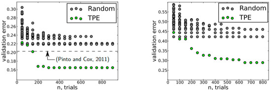
Figure 1.
Comparison of the TPE-optimization and random search validation set performance on the different datasets [15].
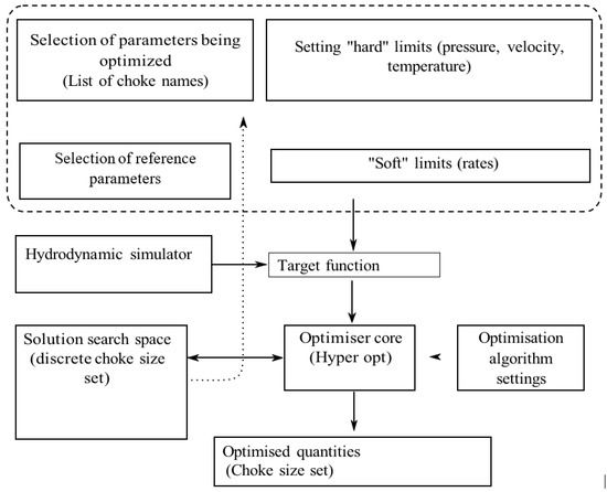
Figure 2.
Diagram of the optimization of the well process conditions.
At the initial stage, the user defines a list of the names of the parameters to be adapted and a list of reference parameters. It is possible to set arbitrary hard limits (using some of the reference parameters). The target function used in the TPE algorithm had access to the hydrodynamic simulator. As a result, the optimizer core obtained the target function and the previously defined solution search space.
The optimization problem can be expressed as:
Here, is the target function; is a set of parameters at which the target function minimum is achieved; is the defined region where the target function parameters reside.
Figure 3 illustrates the functioning of the Bayesian optimization algorithm in a one-dimension case. A surrogate model, being a probabilistic representation of the target function, based on the set of previous observations, was built into each step of the algorithm. Such probabilistic representation of the target function with the use of Gaussian processes is known as kriging or Gaussian process regression. Gaussian processes enable the reconstruction of the behavior of the function with the aid of interpolation and can be extrapolated into regions without known observation points. Adding more observation points provides for a better behavior description of a real target function. With a sufficient number of known values at the points, the optimization using the surrogate model provides good results in a real function. Every evaluation of the real target function provides information in which to build the surrogate probability function with more adequate behavior.
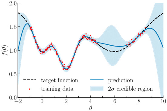
Figure 3.
Illustration of the Gaussian process in a one-dimension case for the target function (dashed line). The training set plus Gaussian noise with an RMS deviation of 0.03 is shown by the red dots. The light blue line shows the mean value predicted by the Gaussian process, and the painted area around it is the 2σ error. The illustration is from [16].
An important advantage of the surrogate model is that it is not necessary to calculate the values of the real target function at multiple intermediate points of the search space. This is particularly convenient when the calculation of such values at each point is associated with substantial time input, as in the case of the calculation of the well’s technical conditions.
Selection of the parameter set may be dictated by the criterion known as the expected improvement or EI.
Here, y* is the threshold value of the target function; y is the values of the real target function subject to the selection of parameters x; p(y|x) is the surrogate representation characterizing the probability of having a y value with the x set. No explicit functional form of p(y) was needed. The ultimate goal is to maximize EI. Further on, we will use the γ parameter that corresponds to y*: p(y < y*) = γ.
If p(y|x) is equal to 0 wherever y < y*, this set of x will not provide a noticeable improvement. If the integral is positive, this set of x will provide better results than the threshold value.
The current implementation has an inherent feature of the possibility of using other algorithms and libraries. Therefore, using the family of evolutionary algorithms, specifically the pygmo library, is an interesting alternative approach.
3. Results
3.1. Well Process Conditions Optimization Algorithm
The optimization module delivers the task of determining the well process conditions that ensure the required value of the target function. The target function in one of the optimization problems can be represented by the final gas rate at the GTF inlet. Additionally, multiple target functions can be handled, which allows for the solving of production problems such as, for instance, maximizing the condensate production at the given level of gas production, or minimizing the water production at a given level of gas production, and so on. The algorithm enables one to set additional boundary conditions including but not limited to pressure, stream velocity, and temperature, and these limitations can be taken into account directly in the target function.
Due to a large number of variables, the problem of optimizing the well process conditions has a large scale. Traditionally, the random search and grid search algorithms have been employed to solve large-scale problems. However, the efficiency of these algorithms is limited to their not using data from previous iterations to identify the most promising parameter region. Unlike random search algorithms, Bayesian optimization algorithms consider a priori information, so they can be broadly used in practical applications related to the development of hydrocarbon fields. In this paper, we used the TPE algorithm (tree-structured Parzen estimator), and the detailed description of its functioning is given in [15]. The algorithm was implemented in the Python Hyperopt library.
3.2. Optimization with Multiple Target Functions
As applied to oil and gas production, the optimization should also consider some process restrictions imposed on the gas transportation system facilities such as pipelines and their connections, wells, chokes, GTF (gas treatment facility), and so on.
As a rule, the minimum pressure is not used, but it can be varied from the GTF upstream pressure to pad the downstream pressure; the minimum bottom hole pressure is not normally used either, but it can be varied from the formation pressure to the GTF upstream pressure.
3.3. Results of Process Conditions Optimization
The results of applying the proposed optimization algorithm can be demonstrated by a pad with 13 wells at a gas condensate field in Western Siberia.
The compositional filtration model is the main model used in the analysis of gas and gas condensate fields with a complex composition of hydrocarbon fractions. Unlike the classical model of the “black” oil type, which contains three phases and three components, the number of fluid components in the compositional model is arbitrary (and in practice numbers several dozen). In this case, the production fluid was given in the form of a compositional model consisting of 10 hydrocarbon components, nitrogen, carbon dioxide, and a small fraction of water. In the available temperature and pressure ranges, it can be presented as a two-phase fluid with a predominant proportion of gas.
In the calculations used in this article, the Beggs–Brill correlation friction model (1973) was used to account for the friction effect of a multiphase flow.
During production at a gas condensate field, one of the optimization tasks can be defined to maximize the rate of liquid hydrocarbons with a set gas rate.
Moreover, the following process limits apply:
In the pipeline:
- -
- Maximum velocity of flow in the pipes: 10 m/s;
- -
- Maximum pipe pressure: 12 MPa.
At GTF:
- -
- Pressure range: 8 to 12 MPa;
- -
- Maximum mass flow rates of gas/condensate/water: 28/15/10 kg/s.
Inside the wells:
- -
- Maximum fluid well head temperature: 20 °C;
- -
- Maximum gas volumetric flow rate: 15 m3/s;
- -
- Maximum mass flow rates of condensate/water: 10/5 kg/s.
At surface chokes:
- -
- Nominal bore range: from 8 mm to 13 mm;
- -
- Maximum number of simultaneous nominal bore changeover: 5.
A delay of several days between the choke nominal bore change in a producing well is an important condition for changing the technical conditions of a producing well. This is essential for achieving a steady-state operation of the well, which ensures its trouble-free operation. Under this condition, a certain time interval was set for the optimization, equal to five days in our case. As per the set time interval, we achieved a three-step optimization of the gas and gas condensate production for a span of 20 days (1 August 2021–20 August 2021). Thus, the process conditions of the wells were changed at the start of the mentioned days: 6 August 2021, 11 August 2021, and 16 August 2021. On day 1, all nominal bores of the surface chokes were set in accordance with the actual parameter chart, and the number of nominal bores that could be changed at the same time was limited at each optimization stage. The choke nominal bores for each day of production are given in the parameter chart (Table 1).

Table 1.
Sample of the restriction ranges for the target function parameters.
All of the wells were adapted from the historical data obtained from the parameter chart of a real field, and afterward, the surface choke nominal bores were slightly altered for the demonstration. With the altered nominal bores of chokes, the production was as follows: 23.479 m3/s DSG, 0.588 m3/s NGL, 4.324 kg/s condensate, with a CGR equal to 0.180 cm3/m3. If the respective process conditions are maintained, the values will gradually drop as the formation depletes.
At each optimization step on 6 August 2021, 11 August 2021 and 16 August 2021, an increase in the condensate production was observed, with the above process limits being met, see Figure 4 and Table 2. For the cumulative production plot, refer to Figure 5. At the end of the optimization period, the gain in condensate production was 106 tons, which was 1.4% more than the production in non-optimized conditions.
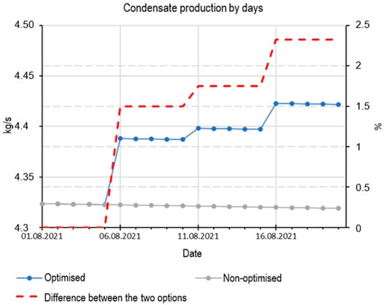
Figure 4.
The simulated condensate production profile during 20 days, as shown by the parameter chart with 3-step optimization. The difference between two options (optimized and non-optimized) as shown by the red dashed line has its own vertical axis on the right side of the plot (percentage points were used here).
Table 2.
Parameter chart for 20 days with the 3-step production optimization.
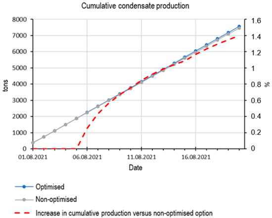
Figure 5.
Cumulative condensate production for 20 days with 3-step optimization. The difference between two options (optimized and non-optimized) shown by the red dashed line has its own vertical axis on the right side of the plot (percentage points were used here).
The goal of the optimization of the well process conditions was to maximize the condensate rate while meeting a number of process limits as above-mentioned. To sum up, it can be concluded that by the end of the 20-day period, the condensate rate rose by 2.3% versus the production in non-optimized conditions.
4. Discussion
This article shows an example of solving an important technological problem using the mathematical optimization process. The solution assumes finding an “instantaneous” (for a short historical period) solution. If we look at the prospect of field development, then the task should be implemented in relation to the underground part of the reservoir. Herewith, for a long historical period, the solution may be differ significantly from the proposed technological scheme. Thus, it is necessary to look for an integrated solution in a bundle − underground part + well + ground infrastructure.
Despite the fact that the used optimization algorithm has a number of advantages and can be applied in a wide range of applications, one important feature is that, in comparison with other optimization algorithms, the TPE optimization does not take into account the rating considerations and selects all wells with equal priority at a time. At each optimization step, the algorithm iterates over the options and starts anew, which is a resource-intensive procedure.
In a solved multifactorial task, TPE optimization can be used in different scenarios; when strict constraints are met, target parameters are achieved. At the same time, the sets of diameters of the chokes may differ significantly. Thus, the implemented algorithm cannot be used in tasks where it is necessary to take into account the previous state. If, for example, we want to limit the frequency of switching on the fittings, then other approaches should be used, for example, group optimization or optimization with guiding bits. In addition, the last two algorithms always found an unambiguous solution, all other things being equal.
In this paper, the technological constraints on the entire system were used as a condition for the objective function. The diameters of the through holes of the fittings varied in a given range of values, without the possibility of its complete disconnection. In a particular case, such functionality was not required, but for large deposits with a changing fluid composition such a possibility may be critical, and will be implemented in further development.
Another assumption used in this work was the use of one fluid model in all wells. The total composition of the extracted fluid differed only due to the different water content in wells with the same composition of the hydrocarbon part. In this paper, it was assumed that the difference in the gas fractions of the hydrocarbon part was due to the different conditions and flow regimes. However, in a real field, the component composition of the fluid from well to well may vary significantly. This assumption did not allow for the detailed adjustment of the calculated debits to the actual data.
It should also be noted that a simplified reservoir model was used in this work. This approach does not take into account the changes in the composition of the reservoir fluid during production; however, it has little effect on the results of the short-term production forecast and significantly simplifies the user’s work.
The developed algorithm currently uses the diameters of the through holes of the fittings as optimized parameters. In the future, the possibility of adjusting the parameters of the ESP, gas lift, etc. will be added, which will allow the developed approach to be used not only for gas and gas condensate wells, but also for oil wells.
The computational cost in terms of the calculation time for the present model was about 30 min, and the technical characteristics were a 8-Core CPU, 3.3 GHz, and 16 GB RAM.
5. Conclusions
This paper developed an estimation algorithm that simulates the flow of multiphase streams in pipes and employs the TPE algorithm to deliver important process engineering tasks related to the optimization of hydrocarbon production. With the operation of a pad with 13 wells at a gas condensate field taken as an example, the task of maximizing the gas condensate production with the defined target function limits was met.
The goal of the optimization of the well process conditions was to maximize the condensate rate while meeting the above-mentioned process limits. With the use of the developed estimation module, the condensate rate increased by 2.3% by the end of the 20 day optimization period. Cumulative condensate production rose by 1.4%, which was 100 + tons versus the non-optimized option.
To sum up, it can be concluded that compared to production in non-optimized conditions, the condensate rate increased, which is what was required. The developed calculation package that combines the physics of the multiphase fluid flow in pipes and the optimization algorithm can boost the performance of the oil and oil and gas fields.
Thus, in this work, it was shown that the use of the created computing software, combining the physics of the flow of multiphase fluid in the pipes and an optimization algorithm, makes it possible to effectively optimize the technological mode of the operation of gas–gas condensate wells. The optimal technological regime, in turn, allows for the efficient development of deposits of liquid and gaseous hydrocarbons.
Author Contributions
A.C.—conceptualization, writing—review and editing; E.U.—methodology, resources, writing—original draft preparation; B.K.—formal analysis; A.K.—investigation; A.V.—data curation, writing—original draft preparation; P.L.—formal analysis, validation; E.K.—original draft preparation, V.U.—resources, supervision; A.P.—writing—review and editing, methodology. All authors have read and agreed to the published version of the manuscript.
Funding
This research received no external funding.
Institutional Review Board Statement
Not applicable.
Informed Consent Statement
Not applicable.
Data Availability Statement
Not applicable.
Conflicts of Interest
The authors declare no conflict of interest.
References
- Guzhov, A.I.; Titov, V.G.; Medvedev, V.F.; Vasiliev, V.A. Collection, Transportation and Storage of Natural Hydrocarbon Gases; Publ. Nedra: Moscow, Russia, 1978; 405p. [Google Scholar]
- Svarovskaya, N.A. Conditioning, Transportation and Storage of Production Fluid; Publ. TPU: Tomsk, Russia, 2004; 268p. [Google Scholar]
- Brill, G.P.; Mukherjee, H. Multiphase Flow in Wells; Institute of Computer Studies: Moscow, Russia; Izhevsk, Russia, 2006; 384p. [Google Scholar]
- Mamaev, V.A.; Odishariya, G.E.; Klapchuk, O.V. Movement of Gas Liquid Mixtures in Pipes; Publ. Nedra: Moscow, Russia, 1978; 270p. [Google Scholar]
- Mamaev, V.A.; Odishariya, G.E.; Semenov, N.I.; Tochigin, A.A. Hydrodynamics of Gas and Liquid Mixtures in Pipes; Publ. Nedra: Moscow, Russia, 1969; 208p. [Google Scholar]
- Klapchuk, O.V. Hydraulic Characteristics of Gas and Liquid Flow in Wells; Publ. Gas Industry: Moscow, Russia, 1981; pp. 32–35. [Google Scholar]
- Badazhkov, D.V.; Golovin, E.D.; Kozlov, M.G.; Kurmangaliev, R.Z.; Lykhin, P.A.; Ulyanov, V.N.; Usov, E.V. Implementing the Method for Calculation of PVT Properties of a Multiphase Multicomponent Fluid. Autom. Remote Control. Commun. Oil Ind. 2021, 2, 24–31. [Google Scholar]
- Lykhin, P.A.; Usov, E.V.; Chukhno, V.I.; Kurmangaliev, R.Z.; Ulyanov, V.N. Movement Simulation of Gas and Liquid Streams in a Directional Well. Autom. Remote Control. Commun. Oil Ind. 2019, 10, 22–27. [Google Scholar]
- Kolchanov, B.A.; Lykhin, P.A.; Usov, E.V.; Chukhno, V.I.; Brylyakova, A.A. Case Study: Prediction the Rate of a Gas Condensate Well Under Various Process Conditions for Validation of the Mathematical Model of a Multiphase Flowmeter. Autom. Remote Control. Commun. Oil Ind. 2020, 12, 49–57. [Google Scholar]
- Pedersen, K.S.; Fredenslund, A.A.G.E. An improved corresponding states model for the prediction of oil and gas viscosities and thermal conductivities. Chem. Eng. Sci. 1987, 41, 182–186. [Google Scholar] [CrossRef]
- Lockhart, R.W.; Martinelli, R.C. Proposed correlation of data for isothermal two-phase, two-component flow in pipes. Chem. Eng. Prog. 1949, 45, 39–48. [Google Scholar]
- Hagedorn, A.R.; Brown, K.E. Experimental study of pressure gradients occurring during continuous two-phase flow in small-diameter vertical conduits. J. Pet. Technol. 1965, 17, 475–484. [Google Scholar] [CrossRef]
- Duns, H., Jr.; Ros, N.C.J. Vertical flow of gas and liquid mixtures in wells. In Proceedings of the 6th World Petroleum Congress, Frankfurt, Germany, 19–26 June 1963. [Google Scholar]
- Orkiszewski, J. Predicting two-phase pressure drops in vertical pipe. J. Pet. Technol. 1967, 19, 829–838. [Google Scholar] [CrossRef]
- Bergstra, J.; Bardenet, R.; Bengio, Y.; Kégl, B. Algorithms for Hyper-Parameter Optimization. Adv. Neural Inf. Process. Syst. 2011. Available online: https://papers.nips.cc/paper/2011/file/86e8f7ab32cfd12577bc2619bc635690-Paper.pdf (accessed on 5 April 2022).
- Leclercq, F. Bayesian optimization for likelihood-free cosmological inference. Phys. Rev. D 2018, 98, 063511. [Google Scholar] [CrossRef] [Green Version]
Publisher’s Note: MDPI stays neutral with regard to jurisdictional claims in published maps and institutional affiliations. |
© 2022 by the authors. Licensee MDPI, Basel, Switzerland. This article is an open access article distributed under the terms and conditions of the Creative Commons Attribution (CC BY) license (https://creativecommons.org/licenses/by/4.0/).