Abstract
A neurofuzzy system is proposed for short-term electric load forecasting. The fuzzy rule base of ReNFuzz-LF consists of rules with dynamic consequent parts that are small-scale recurrent neural networks with one hidden layer, whose neurons have local output feedback. The particular representation maintains the local learning nature of the typical static fuzzy model, since the dynamic consequent parts of the fuzzy rules can be considered as subsystems operating at the subspaces defined by the fuzzy premise parts, and they are interconnected through the defuzzification part. The Greek power system is examined, and hourly based predictions are extracted for the whole year. The recurrent nature of the forecaster leads to the use of a minimal set of inputs, since the temporal relations of the electric load time-series are identified without any prior knowledge of the appropriate past load values being necessary. An extensive simulation analysis is conducted, and the forecaster’s performance is evaluated using appropriate metrics (APE, RMSE, forecast error duration curve). ReNFuzz-LF performs efficiently, attaining an average percentage error of 1.35% and an average yearly absolute error of 86.3 MW. Finally, the performance of the proposed forecaster is compared to a series of Computational Intelligence based models, such that the learning characteristics of ReNFuzz-LF are highlighted.
1. Introduction
Accurate short-term electric load forecasting (STLF) is a challenge to power engineers operating modern Energy Management Systems (EMS). Reliable load forecasts with lead times from a few hours to a week constitute crucial information for an effective operation of EMS with regard to unit commitment, hydro-thermal coordination and interchange evaluation. The highly competitive power market, especially in the present turbulent times, requires accurate forecasts in power demand.
During the last thirty years, Computational Intelligence has become a significant tool in electric load forecasting. The first attempts with feedforward artificial neural networks in the 1990s [1,2,3] were followed by the introduction of static fuzzy and neurofuzzy systems [4,5,6,7]. Support vector machines and support vector regression have provided quite efficient forecasters [8,9,10], while evolutionary computation-based approaches [11,12,13] and mixed schemes have contributed as well [14,15]. Prestigious systems, such as the Adaptive Neuro Fuzzy Inference System (ANFIS) [16], have been employed to STLF [17,18,19] and have contributed to a variety of power systems’ problems [20,21].
The revolution in Computational Intelligence that occurred with the emergence of Deep Learning made an impact in various fields, such as system identification and prediction, pattern recognition, signal and image processing [22,23,24,25]. Such an important breakthrough definitely left its footprint in energy management, wind prediction and power systems [26,27,28,29]. In the field of STLF, in particular, all the well-known deep models (LSTM, recurrent neural networks, CNN) have been applied to this challenging problem, and significant contributions have been made [30,31,32,33,34,35,36,37]. Taking advantage of the available computational resources, these Deep Learning Models have managed to model the electric load time-series effectively.
A key issue on prediction problems is the selection of the input variables and the reduction or transformation of the input vector. In the case of STLF, the potential influential inputs are past load values, temperatures and climate variables, rendering this process crucial. Therefore, any approach that would reduce the burden or alleviate the problem is worth examining.
In view of the above, ReNFuzz-LF (Recurrent Fuzzy model for Load Forecasting) is proposed for short-term electric load forecasting of the Greek power system. The fuzzy rule base comprises rules with dynamic consequent parts that are small-scale recurrent neural networks with one hidden layer, whose neurons have local output feedback. ReNFuzz-LF aims at learning the dynamics of electric load time-series throughout the whole year. The training method applied is Simulated Annealing Dynamic Resilient Propagation (SA-DRPROP), an algorithm designed specifically for recurrent structures, which addresses the inherent disadvantages of standard gradient-based methods. ReNFuzz-LF has a reduced structural complexity compared to other computational intelligence-based approaches and is able to operate with a single input, thus avoiding the use of a feature selection preprocessing stage.
The rest of the paper is organized as follows: In Section 2 the architecture of ReNFuzz-LF is described, and its particular features are discussed. The learning method is detailed in Section 3. Section 4 hosts the experimental analysis. Two neurofuzzy models are examined; the former results from uniform partition of the input space, while the fuzzy rule base of the latter is formed by applying the fuzzy C-means clustering algorithm. A comparative analysis with respectable Computational Intelligence-based approaches is also conducted. From these tests, it becomes evident that ReNFuzz-LF is a promising electric load forecaster, since it exhibits efficient performance, similar or superior to those of its competing rivals, while its structural complexity is significantly reduced. This forecasting efficiency can be attributed to the ability of local feedback connections to identify the temporal relations of the time-series. The concluding remarks are given in Section 5.
2. The Architecture of ReNFuzz-LF
In a classic Takagi–Sugeno–Kang fuzzy model [38], the fuzzy rule base consists of rules that contain fuzzy sets in the premise part, while the consequent parts are linear functions of their inputs. In general, these parts can be any continuous and derivable nonlinear function. ReNFuzz-LF contains fuzzy rules whose consequent parts are small-scale recurrent neural networks. Such a scheme was introduced in [39] for telecommunications data forecasting, and its fuzzy rules for a system of m inputs and a single output are written in the form:
where is the input vector, k represents the sample index and Aj corresponds to the fuzzy set of the j-th input of the particular rule.
The proposed neurofuzzy forecaster has the following structural features:
- The fuzzy rules have static premise parts, which comprise m-dimensional hyper-cells, composed of single-dimension Gaussian membership functions along each input axis:
- The firing strength is calculated as the algebraic product of the Gaussian membership functions.
- The consequent parts of the fuzzy rules are three-layer recurrent neural networks in the form of m–H–1. Such a configuration is shown in Figure 1. The network has internal recurrence, since the outputs of the nodes in the hidden layer are fed back with unit delays (local output unit feedback). There exist no feedback connections of the fuzzy rules’ outputs or external feedback from the network’s output.
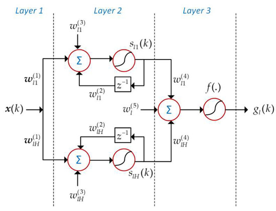 Figure 1. Configuration of the consequent part of a fuzzy rule.The consequent part of the l-th fuzzy rule operates as follows:where:
- ➢
- The hyperbolic tangent is chosen to be the activation function of the neurons, , over other common activation functions, such as sigmoid or rectified linear unit (RELU). As mentioned in [40], the hyperbolic tangent performs better than the logistic sigmoid. In modern deep neural networks, the RELU function is preferred due to the fact that it overcomes the vanishing gradients problem ([40]) that occurs in multilayered networks. In the present case, the consequent parts of the fuzzy rules are too shallow for such a problem to occur. Moreover, the competing rivals of ReNFuzz-LF in Section 4 use the hyperbolic tangent as activation function.
- ➢
- is the output of the i-th hidden neuron of the l-th rule for the k-th sample.
- ➢
- is the output of the l-th fuzzy rule.
- ➢
- , and are the synaptic weights and bias terms, respectively, at the hidden layer of the consequent parts.
- ➢
- and are the synaptic weights and bias terms, respectively, at the output layer of the consequent parts.
- The defuzzification part is static. The output of ReNFuzz-LF is calculated using the weighted average method:
The block diagram of ReNFuzz-LF is hosted in Figure 2.

Figure 2.
Block diagram of ReNFuzz-LF.
The aforementioned architecture falls to a greater category of recurrent neurofuzzy models [41,42], where feedback connections exist at the consequent parts of the fuzzy rules. Among a series of models with external output feedback [43], dynamic premise parts [44] or cascaded recurrent modules [45], ReNFuzz-LF has the advantage of preserving the local-learning character of the classic TSK model. These dynamic consequent parts can be considered as subsystems that are fuzzily interconnected through the defuzzification part. Since the networks are locally recurrent, there is no temporal relation between the rules. At each rule, the fuzzy hypercell of the premise part sets the operating region, while the recurrent consequent part aims to identify, within each region, the temporal dependencies of the internal states of the electric load time-series. The recurrent networks cooperate intrinsically, since the regions are defined in a fuzzy way and overlap each other. Thus, at each data point, usually more than one rules contribute to input–output mapping, leading to enhanced identification capabilities.
The advantages of local output feedback to recurrent neural networks are highlighted in [46,47], where this kind of internal feedback exhibited improved modeling performance in comparison to external feedback or local synapse feedback. Moreover, the neurofuzzy system proposed in [48] was the first approach to introduce internal feedback at the consequent parts of fuzzy rules. However, these parts are highly complex, since they constitute neural networks with Finite Impulse Response and Infinite Impulse Response synapses at the hidden layer, as well as at the output layer. As shown in [39], a simple recurrent structure to the consequent part of the fuzzy rules can perform efficiently with a significantly lower computational burden. In this perspective, ReNFuzz-LF can be regarded as a low-complexity recurrent fuzzy neural model, especially when it is compared to Deep Learning counterparts.
3. The Learning Process
The learning process consists of two parts: structure and parameter identification. Structure identification concerns the selection of the input vector and the determination of the fuzzy rule base. In the case of the Greek Power System, a single input is selected; therefore, a feature selection step is avoided. As far as the fuzzy rule base is concerned, two types of partitions are examined: grid partition and partition based on a clustering algorithm. In the grid partition, the membership functions of the fuzzy sets are uniformly distributed along the input axis, based on a predetermined overlapping coefficient. The size of the rule base is attempted to be kept low, providing economical models. The parameters of the membership functions are extracted automatically: the mean values depend on the number of fuzzy sets and the range of the input space, while the standard deviations are common to all fuzzy sets and depend on the overlapping coefficient.
Partition based on a clustering algorithm provides the most appropriate fuzzy sets in terms of minimum distances between the data samples that belong to each cluster, thus producing fuzzy rules that each one of them is focused on a part of the data set. The algorithm employed is the fuzzy C-means (FCM), which was defined by Dunn [49] and developed by Bezdek in [50,51]. It belongs to a broad class of geometrical fuzzy clustering algorithms as reported in [52]. For a given number of clusters, R, the cluster centers of a multidimensional data set are calculated by the following formula:
where N is the number of samples, and denotes the membership degree that belongs to the l-th cluster:
c is a scale parameter within [0, 1].
The cluster centers correspond to the mean values of the Gaussian membership functions. The standard deviations are derived according to [53]:
A key issue in the model building stage when a clustering algorithm is involved, is the selection of the number of clusters, which is the number of fuzzy rules. Since the correct partition is not known a priori, internal validation methods should be applied. As reported in the review work on cluster validity indices in [54], the Davies–Bouldin index [55] constitutes a well-known efficient internal validation method. The DB index depends on the separation of the clusters and the compactness of each cluster; therefore, it favors clusterings with high separation values and reduced scattering of the points that belong to a cluster. The lower the values of the DB index, the better the resulting clustering.
In both the aforementioned cases of partition, once the fuzzy sets are determined, the premise part parameters remain fixed. Thus, the weights of the neural consequent parts are calculated in the sequel.
The tuning algorithm for the synaptic weights should take into consideration the recurrent nature of the consequent parts of the fuzzy rules; therefore, it should be able to handle the time dependencies that the feedback loop at each hidden neuron creates. In this perspective, the Simulated Annealing Dynamic Resilient Propagation (SA-DRPROP, [56]) is employed. SA-DRPROP efficiently deals with the problem of trapping to local minima, which is common to gradient-based learning methods. The introduction of Simulated Annealing, however, aims to perform a search for the optimal weights at a broader weight space. The training method is an iterative algorithm based on SARPROP [57], which was designed for static neural networks and is fully adapted to the architecture of ReNFuzz-LF.
Let be one of the consequent synaptic weights in Equations (4) and (5). For the present and previous iterations of SA-DRPORP, t and t-1, respectively, let , be the partial derivatives of an error function E with respect to the adaptive weight . At each iteration, each weight is updated using its own step size. Moreover, the step size is adjusted according to the sign of the respective derivative at the current and the previous iterations. Therefore, the size of the gradient is not taken into consideration, a common practice to gradient-based methods, and only the temporal behavior of the gradient matters. Using pseudo-code, the algorithm is summarized as follows (Algorithm 1):
| Algorithm 1. SA-DRPROP | ||
| 1: | (a)Initialize the step sizes of the consequent weights : | |
| 2: | Repeat | |
| 3: | (b) For each weight , compute the SA-DRPROP error gradient: | |
| 4: | ||
| 5: | (c) For each weight , update its step size: (c.1) If | |
| 6: | Then, | |
| 7: | (c.2) Else, if | |
| 8: | Then, | |
| 9: | If | |
| 10: | Then | |
| 11: | Else, | |
| 12: | (c.3) Else, | |
| 13: | Update : | |
| 14: | Until convergence | |
Initially, the step size takes a moderate value, , and at each iteration it is updated according to the sign of the error gradient. At the initial stages of the training process, when the error keeps reducing, step c1 leads to an increase in the step size by , in order to accelerate learning. At later stages, c2 becomes effective, and the step size is decreased by an attenuation factor in order to avoid oscillations. Moreover, all the step sizes are bounded by such that minima will not be missed, and by to ensure that learning will not be stalled.
In SA-DRPROP, the notion of simulated annealing is implemented at steps (b) and (c2). At step (b), a weight decay term is added to the error gradient. Therefore, in the beginning of the learning process, weights with lower values are favored. As training proceeds, this decay term diminishes, thus allowing the increase in bigger weights and facilitating the exploration of areas of the error surface that were previously unavailable.
At step (c2), noise is added to the weight update value when the sign of the error gradient is changed, and the magnitude of the update value is less than threshold, which is proportional to the square of the SA term (). Therefore, the adaptation process is moderately affected, since the modification of the weight update by noise takes place only when the weight is threatened to fall to a local minimum, thus allowing the weight to overcome this minimum.
Parameter r affects the noise level and takes random values within [0, 1], (Temp is the temperature), is set to a small number (e.g., 0.01) and is set around 0.5.
The derivatives are the standard partial derivatives for those consequent weights that are not involved in the recurrent loop, and are derived by use of the classic chain rule:
where is the derivative of , with respect to its arguments, and is the actual load value.
For the weights of the hidden layer’s recurrent neurons, the use of ordered derivatives is necessary in order to unfold in time the neuron’s operation [58]. Moreover, Lagrange multipliers are introduced, which facilitate the calculation of the error gradients [59].
Let be one of the consequent synaptic weights of the l-th fuzzy rule in Equations (4) and (5). The ordered derivative of Ε with respect to is provided by the following formula:
Applying Lagrange multipliers to Equation (12) in order to facilitate calculation of , the error gradients are extracted as follows:
Equation (16) is a backward difference equation: first, the boundary conditions in Equation (17) for are calculated, and then, the Lagrange multipliers are extracted in a backward manner for .
4. Experimental Results
4.1. Problem Statement—Data Preprocessing
ReNFuzz-LF is applied to the problem of forecasting the next day’s hourly loads of the Greek Interconnected Power System. In particular, a single fuzzy model is generated to perform hourly based load forecasting of the whole year, including weekends and holidays.
One of the most important tasks in building an efficient electric load forecaster is the feature selection step, where the most relevant input variables that highly affect the forecaster’s output are extracted. This is a cumbersome activity due to the complicated nature of the process. Selecting a wrong input set may lead to models with poor forecasting performance. Unfortunately, there is no systematic procedure that can be followed in all circumstances. In certain cases, input selection is heuristically performed or based on the expertise provided by the system operators. However, several statistical methods such as auto-correlation and cross-correlation have been successfully applied in the literature. Furthermore, well-known concepts of the linear regression theory can also be employed. As mentioned in Section 1, in general the input candidates can be divided into three major groups: electric load variables, temperature variables and climate variables. A large variety of these variables are reported in the literature, including their daily means and lagged hourly values up to 3 weeks back [35].
The suggested modeling approach does not face this issue at all, single ReNFuzz-LF is a single-input forecaster. Therefore, having as a single input the actual load at hour h of day d−1, (MW), ReNFuzz-LF predicts the load at the same hour of day d, thus performing the mapping:
where d = 1,...,365 is the day index and h = 1,...,24 is the hour index. A hat (^) above a variable indicates the actual quantity. The intrinsic dependence on past loads is attempted to be modeled through the feedback loops at the consequent parts of the fuzzy rules. The effect of temperature or climate variables has not been studied in this work since our goal is to keep the input vector and the model’s complexity to a minimum.
The scope of the identification process is to develop and train a neurofuzzy model that is capable of performing the input–output matching of the available data to an acceptable level of accuracy. The average percentage error with respect to the daily peak (APE) is selected as an error measure to evaluate the model’s forecasting performance. The APE is defined as follows:
where N is the number of days in the data set and is the maximum actual load of day d.
The data set contains 35,064 data and is split to training and testing data sets, with a ratio of 75/25%, respectively. The training data set is used during the identification process. It contains 26,280 samples, which are historical data from three consecutive years (2013–2015). The evaluation set, used for testing the forecasting capabilities of ReNFuzz-LF, contains 8784 samples of electric load values for 2016 (a leap year, containing 366 days). The data are publicly available at the website of the Greek Independent Power Transmission Operator [60]. There were some missing or irregular values; therefore, a data preprocessing phase took place for data cleaning, data integration and data normalization. In particular, a data file of 25 columns (one for the data and twenty-four for the hourly loads) and 1461 lines (three regular years and one leap year) was created.
Missing values were filled by the average of the value at the same hour of most previous date and the next one. In the case of consecutive missing values, they were filled by cubic spline interpolation. Irregular values were substituted in the same way.
Data were normalized within , such that load values fall within the operating region of the neurons at the consequent parts of the fuzzy rules. Moreover, the data file was enriched with metadata (day of the week, season of the year), such that further tests and evaluation based on various data selection criteria could take place.
4.2. ReNFuzz-LF’s Structural and Parameter Characteristics
The number of hidden neurons for the consequent part of the fuzzy rules is set to 2, leading to a 1–2–1 recurrent neural network. Structures with hidden layers containing up to eight neurons were examined in order to combine accurate predictions with moderate complexity of the forecaster, thus facilitating its implementation and reducing training time. Bigger networks slightly improved the forecasting performance for the testing data set, while hidden layers of more than six neurons led to overfitting.
In the case of grid partition, fuzzy rules bases varying from 3 to 12 rules were examined, and the resulting rule base contains six rules, leading to a model of 66 parameters, as shown in Table 1. Overlapping coefficients between consecutive fuzzy sets is set to 0.35, in order to have an efficient coverage of the input space by more than one rule, while avoiding the mixing of rules to a great extent.

Table 1.
Premise and consequent parameters (weights) of ReNFuzz-LF.
In order to perform partition by means of FCM, the Davies–Bouldin index, shown in Figure 3, was examined. It is evident that the first minimum is attained for three clusters and that the index starts taking lower values after the seventh cluster. However, compared to a three-rule model, the forecasters with bigger fuzzy rule bases do not provide ameliorated performances with regard to the testing data; on the contrary, models with more than seven rules suffer from overfitting. Therefore, since one of the primary goals is a reduced computational cost, a ReNFuzz-LF with fuzzy rules and 33 parameters is selected, a reduction by 50% with respect to grid partition, which underlines the benefit from searching the input space for appropriate clusters. This partition is depicted in Figure 4.
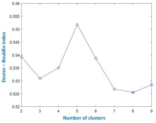
Figure 3.
The Davies–Bouldin index.
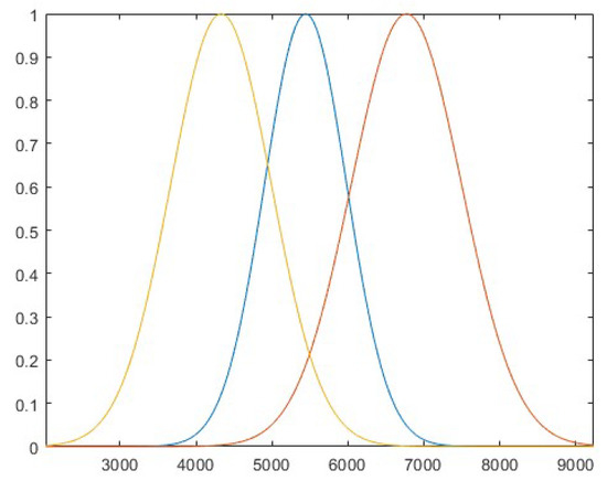
Figure 4.
Input space partition by FCM.
Once the fuzzy sets are defined, the premise parameters are set and are not adaptable, both in grid partition and in partition by FCM. Thus, only the consequent parameters (82% of the total number of parameters) are updated by the iterative algorithm SA-DRPROP.
Training lasts for 1000 epochs. The error measure selected for the extraction of the error gradient is Root Mean Squared Error (RMSE), which is also a performance metric:
The RMSE measures, in a quadratic manner, the discrepancy between the actual data series and the one produced by ReNFuzz-LF. Hence, it will serve as an evaluation criterion complementary to APE.
The learning parameters of SA-DRPROP are shown in Table 2.
Table 2.
Learning parameters of SA-DRPROP.
4.3. Results and Discussion
The performance of ReNFuzz-LF for short-term electric load forecasting is evaluated in the sequel. Table 3 summarizes the yearly forecast APE and RMSE for the two forecasters with different partitions. APE values below a threshold of 2% correspond to reliable load prediction. Although a single model is used for the whole year, seasonal forecasting results for the best model (which will be used in the sequel) are shown in Table 4 in order to investigate whether ReNFuzz-LF is capable of identifying the seasonal electric load profiles.
Table 3.
Yearly APE and RMSE.
Table 4.
Seasonal APE and RMSE for FCM ReNFuzz-LF.
The average yearly absolute error for the testing data set is 86.3 MW, and the respective standard deviation is 86.8 MW, which means that the forecast error is less than 173 MW for most of the 8784 h (366 days of 2016). The forecast error duration curve is shown in Table 5. It represents the percentage of hours of the year in which the forecast error is greater than the MW value given in the first row. It can be easily observed that for 68% of the time the forecast error is less than 100 MW. Additionally, only 0.45% of the time does the forecast error exceed 500 MW.
Table 5.
Forecast error duration curve for FCM ReNFuzz-LF.
The performance of the forecast model is further examined through a series of graphs regarding all seasons. In particular, in Figure 5, Figure 6, Figure 7 and Figure 8, the times series of the actual and the predicted loads for weekdays and Sundays are depicted.
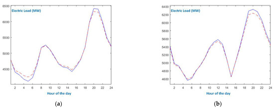
Figure 5.
Presentation of winter days. The blue solid line is the actual electric load, and the red dotted line is ReNFuzz-LF’s output: (a) working day; (b) Sunday.
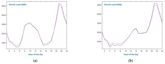
Figure 6.
Presentation of spring days. The blue solid line is the actual electric load, and the red dotted line is ReNFuzz-LF’s output: (a) working day; (b) Sunday.
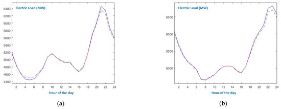
Figure 7.
Presentation of summer days. The blue solid line is the actual electric load, and the red dotted line is ReNFuzz-LF’s output: (a) working day; (b) Sunday.
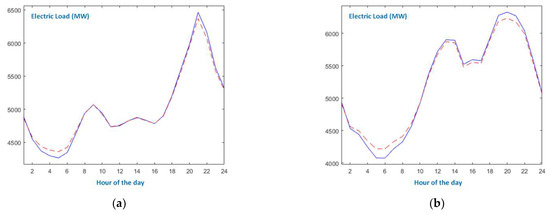
Figure 8.
Presentation of autumn days. The blue solid line is the actual electric load, and the red dotted line is ReNFuzz-LF’s output: (a) working day; (b) Sunday.
According to the graphs, the following comments are in order:
- The working days of the four seasons bear similarity with respect to the appearances of morning and evening peaks, as well the first minimum load. As far as the load evolution during the day is concerned, autumn working day is smoother from 10 a.m. to 4 p.m.
- Sundays exhibit different patterns compared to their respective working days. Moreover, they differ considerably from season to season. It is evident that spring and autumn Sundays follow the respective seasonal pattern only during late evening and around midnight.
- Despite the differences in seasonal behavior and in the type of days, ReNFuzz-LF succeeds in tracking the actual time-series at all times. Maximum and minimum extremes are identified, and the transition from working days to weekend days is effectively modeled, as can be clearly seen in Figure 9, where a winter week is shown.
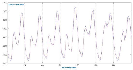 Figure 9. A winter week. Blue solid line: actual electric load. Red dotted line: ReNFuzz-LF’s output.
Holidays are an interesting type of day, such as Christmas. In Greece, a special summer holiday is August 15th (Assumption day). The electric load curves for these two holidays are given in Figure 10. It is concluded that ReNFuzz-LF identifies the Christmas load curve efficiently, since it is similar to winter Sundays. However, it fails to track load evolution of Assumption Day, at least until 6 p.m. The load curve of this day is highly irregular: for the first 18 h, there is no morning peak, and load is reducing, leading to a minimum below 3000 MW around 3 p.m. (lunch time). This behavior can be attributed to the fact that during this particular day, the vast majority of Greek people are on holiday and do not stay at home. They spend the morning at the beach and do not return to their summer houses or to hotels until late evening. Moreover, around Assumption day, no industrial activity takes place, due to August holidays. It can be seen that the evening and night parts of the time-series regain their “normal” nature, and the forecaster performs accurate predictions accordingly.
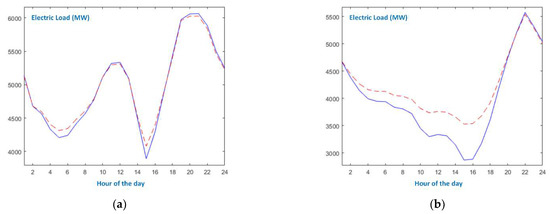
Figure 10.
Presentation of holidays. The blue solid line is the actual electric load, and the red dotted line is ReNFuzz-LF’s output: (a) Christmas day; (b) Assumption day.
The suggested neurofuzzy recurrent model is now compared with three Computational Intelligence-based models reported in the literature, namely, ANFIS [16], LSTM forecaster [30,35] and the DFNN neurofuzzy model [48]. ANFIS is the most well-known neurofuzzy system, LSTM is a popular and effective Deep Learning model, while DFNN constitutes a system that shares the same underlying philosophy with ReNFuzz-LF but is more complex. Comparison of the forecasters is attempted in terms of forecasting accuracy and the number of total parameters. For fair comparison, all models are evaluated using the same data sets. Four setups of the LSTM scheme are examined: networks with one and two layers, each layer comprising 25 and 50 units. As far as the other hyperparameters are concerned, they are summarized in Table 6, where the structural and learning parameters of DFNN are also given. The same FCM partition applied to ReNFuzz-LF is used for DFNN. With regard to ANFIS, since the network is static, the input vector is two-dimensional, . Several fuzzy rule bases were investigated, and the one chosen contains 81 rules (nine fuzzy sets per input). The results are shown in Table 7.
Table 6.
Parameters of competing forecasters.
Table 7.
Comparative results.
It is concluded from the results that all four models attained low APE values; therefore, they effectively perform electric load predictions. ReNFuzz-LF and DFNN exhibit a similar performance, leading to the conclusion that the fuzzy blending of locally recurrent small-scale neural networks can efficiently identify the temporal relations of electric load time-series. As far as LSTM models are concerned, those with 25 units exhibit the worst performance, and it takes two 50-unit layers for the performance to be competitive to ReNFuzz-LF’s. In terms of model size and structural complexity, the superiority of the neurofuzzy approach is evident. ReNFuzzy-LF and DFNN require only a fraction of parameters that LSTM models do, while ANFIS has eight times more parameters than the proposed forecaster. Additionally, ReNFuzz-LF is quite more economical than DFNN, both in terms of parameter set and algorithmic complexity.
Summarizing, apart from the significantly low APE that ReNFuzz-LF attained and the reduced model complexity, the proposed forecasting approach displays some additional advantages:
- The usual selection process with regard to past load values is skipped. No dimensionality reduction is necessary, which adds additional cost to the preprocessing phase. The internal dependencies of the time-series are identified through the recurrent processing that the consequent parts of the fuzzy rules perform.
- The model does not make use of climate data, such as temperature of humidity.
- No seasonal models or models dependent on the nature of the day (weekday, weekend, holiday) are necessary. With the exemption of August 15th, ReNFuzz-LF succeeded in predicting the electric load of irregular days quite accurately.
5. Conclusions
A dynamic neurofuzzy model for short-term electric load forecasting has been proposed. ReNFuzz-LF is a fuzzy system with rules that have nonlinear dynamic consequent parts, constituting small-scale recurrent neural networks with local output feedback. Training of the consequent parameters is performed via SA-DRPROP. The forecaster has been tested on load time-series from the Greek power system, exhibiting an efficient prediction, compared to a series of Computational Intelligence models. Moreover, ReNFuzz-LF has a moderate model structure since the existence of internal feedback connections are capable of capturing the dynamics of the time-series. As far as future work is concerned, structure learning and parameter tuning by use of evolutionary computation methods are two steps toward a fully automated model building process.
Author Contributions
Conceptualization, G.K., P.M. and A.V.; methodology, G.K., P.M., and A.V.; software, G.K. and P.M.; validation, G.K. and A.V.; formal analysis, G.K., P.M. and A.V.; investigation, G.K. and P.M; resources, G.K. and P.M.; data curation, G.K.; writing—original draft preparation, G.K., P.M. and A.V.; writing—review and editing, P.M. and A.V.; visualization, G.K. and P.M.; supervision, P.M.; project administration, P.M. All authors have read and agreed to the published version of the manuscript.
Funding
This research received no external funding.
Data Availability Statement
Publicly available datasets were analyzed in this study. This data can be found here: https://www.admie.gr/en/market/market-statistics/detail-data/ (accessed on 10 April 2022).
Conflicts of Interest
The authors declare no conflict of interest.
Nomenclature
| membership function of the i-th input axis for the l-th fuzzy rule | |
| mean of a Gaussian membership function of the i-th input axis for the l-th fuzzy rule | |
| standard deviation of a Gaussian membership function of the i-th input axis for the l-th fuzzy rule | |
| H | number of hidden neurons |
| RMSE | root mean squared error |
| APE | average percentage error |
| n | number of samples |
| FIR | finite impulse response |
| IIR | infinite impulse response |
| maximum electric actual load of day d | |
| actual electric load at hour h of day d-1 | |
| the output of the i-th hidden neuron of the l-th fuzzy rule | |
| the output of the l-th fuzzy rule | |
| synaptic weights at the hidden layer of the fuzzy rules | |
| bias terms at the hidden layer of the fuzzy rules | |
| synaptic weights at the output layer of the fuzzy rules | |
| bias terms at the output layer of the fuzzy rules | |
| membership degree that a sample belongs to the l-th cluster (FCM) | |
| c | scale parameter (FCM) |
| ordered partial derivative of an error measure with respect to a consequent weight | |
| Lagrange multiplier | |
| actual electric load value | |
| increase factor for step size | |
| attenuation factor for step size | |
| r | scale parameter for noise (SA-DRPROP) |
| Temp | temperature (SA-DRPROP) |
| Scale coefficients for SA term (SA-DRPROP) | |
| minimum step size | |
| maximum step size | |
| initial step size |
References
- Park, D.C.; El-Sharkawi, M.; Marks, R.; Atlas, L.; Damborg, M. Electric load forecasting using an artificial neural network. IEEE Trans. Power Syst. 1991, 6, 442–449. [Google Scholar] [CrossRef] [Green Version]
- Papalexopoulos, A.; How, S.; Peng, T. An implementation of a neural network based load forecasting model for the EMS. IEEE Trans. Power Syst. 1994, 9, 1956–1962. [Google Scholar] [CrossRef]
- Bakirtzis, A.; Theocharis, J.; Kiartzis, S.; Satsios, K. Short term load forecasting using fuzzy neural networks. IEEE Trans. Power Syst. 1995, 10, 1518–1524. [Google Scholar] [CrossRef]
- Mastorocostas, P.; Theocharis, J.; Bakirtzis, A. Fuzzy modeling for short term load forecasting using the orthogonal least squares method. IEEE Trans. Power Syst. 1999, 14, 29–36. [Google Scholar] [CrossRef]
- Papadakis, S.; Theocharis, J.; Bakirtzis, A. A load curve based fuzzy modeling technique for short-term load forecasting. Fuzzy Sets Syst. 2003, 135, 279–303. [Google Scholar] [CrossRef]
- Bansal, R. Bibliography on the fuzzy set theory applications in power systems. IEEE Trans. Power Syst. 2003, 18, 1291–1299. [Google Scholar] [CrossRef]
- Dash, P.; Liew, A.; Rahman, S.; Dash, S. Fuzzy and neuro-fuzzy computing models for electric load forecasting. Eng. Appl. Artif. Intell. 1995, 8, 423–433. [Google Scholar] [CrossRef]
- Chen, B.; Chang, M. Load forecasting using support vector machines: A study on EUNITE competition 2001. IEEE Trans. Power Syst. 2004, 19, 1821–1830. [Google Scholar] [CrossRef] [Green Version]
- Ghelardoni, L.; Ghio, A.; Anguita, D. Energy load forecasting using empirical mode decomposition and support vector regression. IEEE Trans. Smart Grid 2013, 4, 549–556. [Google Scholar] [CrossRef]
- Yang, A.; Li, W.; Yang, X. Short-term electricity load forecasting based on feature selection and least squares support vector machines. Knowl. Based Syst. 2019, 163, 159–173. [Google Scholar] [CrossRef]
- Giasemidis, G.; Haben, S.; Lee, T.; Singleton, C.; Grindrod, P. A genetic algorithm approach for modelling low voltage network demands. Appl. Energy 2017, 203, 463–473. [Google Scholar] [CrossRef] [Green Version]
- Yang, X.; Yuan, J.; Yuan, J.; Mao, H. An improved WM method based on PSO for electric load forecasting. Expert Syst. Appl. 2010, 37, 8036–8041. [Google Scholar] [CrossRef]
- Dudek, G. Artificial immune system with local feature selection for short-term load forecasting. IEEE Trans. Evol. Comput. 2017, 21, 116–130. [Google Scholar] [CrossRef]
- Li, S.; Wang, P.; Goel, L. A novel wavelet-based ensemble method for short-term load forecasting with hybrid neural networks and feature selection. IEEE Trans. Power Syst. 2016, 31, 1788–1798. [Google Scholar] [CrossRef]
- Zhou, M.; Jin, M. Holographic ensemble forecasting method for short-term power load. IEEE Trans. Smart Grid 2019, 10, 425–434. [Google Scholar] [CrossRef]
- Jang, J.-S.R. ANFIS: Adaptive-network-based fuzzy inference system. IEEE Trans. Syst. Man, Cybern. 1993, 23, 665–685. [Google Scholar] [CrossRef]
- Khan, A.; Rizwan, M. ANN and ANFIS Based Approach for Very Short Term Load Forecasting: A Step Towards Energy Management System. In Proceedings of the 8th International Conference on Signal Processing and Integrated Networks, Noida, India, 26–27 August 2021. [Google Scholar]
- Elkazaz, M.; Sumner, M.; Thomas, D. Real-time energy management for a small scale PV-battery microgrid: Modeling, design, and experimental verification. Energies 2019, 12, 2712. [Google Scholar] [CrossRef] [Green Version]
- Shah, S.; Nagraja, H.; Chakravorty, J. ANN and ANFIS for short term load forecasting. Eng. Technol. Appl. Sci. Res. 2018, 8, 2818–2820. [Google Scholar] [CrossRef]
- Krzywanski, J.; Grabowska, K.; Sosnowski, M.; Zylka, A.; Szteklr, K.; Kalawa, W.; Wojcik, T.; Nowak, W. An adaptive neuro-fuzzy model of a re-heat two-stage adsorption chiller. Therm. Sci. 2019, 23, S1053–S1063. [Google Scholar] [CrossRef] [Green Version]
- Lasheen, M.; Abdel-Salam, M. Maximum power point tracking using hill climbing and ANFIS techniques for PV applications: A review and a novel hybrid approach. Energy Convers. Manag. 2018, 171, 1002–1019. [Google Scholar] [CrossRef]
- Karim, F.; Majumdar, S.; Darabi, H.; Harford, S. Multivariate LSTM-FCNs for time series classification. Neural Netw. 2019, 116, 237–245. [Google Scholar] [CrossRef] [PubMed] [Green Version]
- Demir, F. DeepCoroNet: A deep LSTM approach for automated detection of COVID-19 cases from chest X-ray images. Appl. Soft Comput. 2021, 103, 107160. [Google Scholar] [CrossRef] [PubMed]
- Wang, M.; Lin, T.; Jhan, K.; Wu, S. Abnormal event detection, identification and isolation in nuclear power plants using LSTM networks. Prog. Nucl. Energy 2021, 140, 103928. [Google Scholar] [CrossRef]
- Tsakiridis, N.; Keramaris, K.; Theocharis, J.; Zalidis, G. Simultaneous prediction of soil properties from VNIR-SWIR spectra using a localized multi-channel 1-D convolutional neural network. Geoderma 2020, 367, 114208. [Google Scholar] [CrossRef]
- Massaoudi, M.; Chihi, I.; Abu-Rub, H.; Refaat, S.; Oueslati, F. Convergence of photovoltaic power forecasting and deep learning: State-of-art review. IEEE Access. 2021, 9, 136593–136615. [Google Scholar] [CrossRef]
- Agga, A.; Abbou, A.; Labbadi, M.; El Houm, Y.; Ali, I. CNN-LSTM: An efficient hybrid deep leanring architecture for predicting short-term photovoltaic power production. Electr. Power Syst. Res. 2022, 208, 107908. [Google Scholar] [CrossRef]
- Skrobek, D.; Krzywanski, J.; Sosnowski, M.; Kulakowska, A.; Zylka, A.; Grabowska, K.; Ciesielska, K.; Nowak, W. Prediction of sorption processes using the deep learning methods. Energies 2020, 13, 6601. [Google Scholar] [CrossRef]
- Gao, Z.; Hu, S.; Sun, H.; Liu, J.; Zhi, Y.; Li, J. Dynamic state estimation of new energy power systems considering multi-level false data identification based on LSTM-CNN. IEEE Access. 2021, 9, 142411–142424. [Google Scholar] [CrossRef]
- Veeramsetty, V.; Chandra, D.R.; Salkuti, S.R. Short-term electric power load forecasting using factor analysis and long short-term memory for smart cities. Int. J. Circuit Theory Appl. 2021, 49, 1678–1703. [Google Scholar] [CrossRef]
- Kong, W.; Dong, Z.; Jia, Y.; Hill, D.; Xu, Y.; Zhang, Y. Short-term residential load forecasting based on LSTM recurrent neural network. IEEE Trans. Smart Grid 2019, 10, 844–851. [Google Scholar] [CrossRef]
- Han, L.; Peng, Y.; Li, Y.; Yong, B.; Zhou, Q.; Shu, L. Enhanced deep networks for short-term and medium-term load forecasting. IEEE Access 2018, 7, 4045–4055. [Google Scholar] [CrossRef]
- Bedi, J.; Toshniwal, D. Deep learning framework to forecast electricity demand. Appl. Energy 2019, 238, 1312–1326. [Google Scholar] [CrossRef]
- He, W. Load forecasting via deep neural networks. Procedia Comput. Sci. 2017, 122, 308–314. [Google Scholar] [CrossRef]
- Veeramsetty, V.; Chandra, D.R.; Grimaccia, F.; Mussetta, M. Short term electric load forecasting using principal component analysis and recurrent neural networks. Forecasting 2022, 4, 149–164. [Google Scholar] [CrossRef]
- Eskandari, H.; Imani, M.; Moghaddam, M. Convolutional and recurrent neural network based model for short-term load forecasting. Electr. Power Syst. Res. 2021, 195, 107173. [Google Scholar] [CrossRef]
- Sheng, Z.; Wang, H.; Chen, G.; Zhou, B.; Sun, J. Convolutional residual network to short-term load forecasting. Appl. Intell. 2021, 51, 2485–2499. [Google Scholar] [CrossRef]
- Takagi, T.; Sugeno, M. Fuzzy identification of systems and its applications. IEEE Trans. Syst. Man Cybern. 1985, 15, 116–132. [Google Scholar] [CrossRef]
- Mastorocostas, P.; Hilas, C. ReNFFor: A recurrent neurofuzzy forecaster for telecommunications data. Neural Comput. Appl. 2013, 22, 1727–1734. [Google Scholar] [CrossRef]
- Goodfellow, I.; Bengio, J.; Courville, A. Deep Learning; The MIT Press: Cambridge, MA, USA, 2017; pp. 187–189. [Google Scholar]
- Shihabudheen, K.; Pillai, G. Recent advances in neuro-fuzzy system: A Survey. Knowl. Based Syst. 2018, 152, 136–162. [Google Scholar] [CrossRef]
- Ojha, V.; Abraham, A.; Snasel, V. Heuristic design of fuzzy inference systems: A review of three decades of research. Eng. Appl. Artif. Intel. 2019, 85, 845–864. [Google Scholar] [CrossRef] [Green Version]
- Jassar, S.; Liao, Z.; Zhao, L. A recurrent neuro-fuzzy system and its application in inferential sensing. Appl. Soft Comput. 2011, 11, 2935–2945. [Google Scholar] [CrossRef]
- Juang, C.-F.; Lin, Y.-Y.; Tu, C.-C. A recurrent self-evolving fuzzy neural network with local feedbacks and its application to dynamic system processing. Fuzzy Sets Syst. 2010, 161, 2552–2568. [Google Scholar] [CrossRef]
- Stavrakoudis, D.; Theocharis, J. Pipelined recurrent fuzzy networks for nonlinear adaptive speech prediction. IEEE Trans. Syst. Man Cybern. B. Cybern. 2007, 37, 1305–1320. [Google Scholar] [CrossRef] [PubMed]
- Mandic, D.; Chambers, J. Recurrent Neural Networks for Prediction: Learning Algorithms, Architectures and Stability; John Wiley & Sons, Inc.: Hoboke, NJ, USA, 2001. [Google Scholar]
- Tsoi, A.; Back, A. Locally recurrent Ggobally feedforward networks: A critical review of architectures. IEEE Trans. Neural Netw. 1994, 5, 229–239. [Google Scholar] [CrossRef]
- Mastorocostas, P.; Theocharis, J. A Recurrent fuzzy neural model for dynamic system identification. IEEE Trans. Syst. Man Cybern. B. Cybern. 2002, 32, 176–190. [Google Scholar] [CrossRef]
- Dunn, J. A fuzzy relative of the ISODATA process and its use in detecting compact, well-separated clusters. J. Cybernet. 1974, 3, 32–57. [Google Scholar] [CrossRef]
- Bezdek, J. Fuzzy Mathematics in Pattern Recognition. Ph.D. Thesis, Cornell University, Ithaca, NY, USA, 1973. [Google Scholar]
- Bezdek, J. Cluster validity with fuzzy sets. J. Cybernet. 1973, 3, 58–73. [Google Scholar] [CrossRef]
- Wingham, M. Geometrical fuzzy clustering algorithms. Fuzzy Sets Syst. 1983, 10, 271–279. [Google Scholar] [CrossRef]
- Zhou, T.; Chung, F.-L.; Wang, S. Deep TSK fuzzy classifier with stacked generalization and triplely concise interpretability guarantee for large data. IEEE Trans. Fuzzy Syst. 2017, 25, 1207–1221. [Google Scholar] [CrossRef]
- Arbelaitz, O.; Gurrutxaga, I.; Muguerza, J.; Perez, J.; Perona, I. An extensive comparative study of cluster validity indices. Pattern Recognit. 2013, 46, 243–256. [Google Scholar] [CrossRef]
- Davies, D.; Bouldin, D. A clustering separation measure. IEEE Trans. Pattern Anal. Mach. Intell. 1979, 1, 224–227. [Google Scholar] [CrossRef] [PubMed]
- Mastorocostas, P.; Rekanos, I. Simulated Annealing Dynamic RPROP for Training Recurrent Fuzzy Systems. In Proceedings of the 14th IEEE International Conference on Fuzzy Systems, Reno, NV, USA, 22–25 May 2005. [Google Scholar]
- Treadgold, N.; Gedeon, T. Simulated annealing and weight decay in adaptive learning: The SARPROP algorithm. IEEE Trans. Neural Netw. 1998, 9, 662–668. [Google Scholar] [CrossRef] [PubMed]
- Werbos, P. Beyond Regression: New Tools for Prediction and Analysis in the Behavioral Sciences. Ph.D. Thesis, Harvard University, Cambridge, MA, USA, 1974. [Google Scholar]
- Piche, S. Steepest descent algorithms for neural network controllers and filters. IEEE Trans. Neural Netw. 1994, 5, 198–212. [Google Scholar] [CrossRef] [PubMed]
- Greek Independent Power Transmission Operator. Available online: https://www.admie.gr/en/market/market-statistics/detail-data (accessed on 10 April 2022).
Publisher’s Note: MDPI stays neutral with regard to jurisdictional claims in published maps and institutional affiliations. |
© 2022 by the authors. Licensee MDPI, Basel, Switzerland. This article is an open access article distributed under the terms and conditions of the Creative Commons Attribution (CC BY) license (https://creativecommons.org/licenses/by/4.0/).