Forecasting Regional Carbon Prices in China Based on Secondary Decomposition and a Hybrid Kernel-Based Extreme Learning Machine

Abstract

Accurately forecasting carbon prices is key to managing associated risks in the financial market for carbon. To this end, the traditional strategy does not adequately decompose carbon prices, and the kernel extreme learning machine (KELM) with a single kernel function struggles to adapt to the nonlinearity, nonstationarity, and multiple frequencies of regional carbon prices in China. This study constructs a model, called the VMD-ICEEMDAN-RE-SSA-HKELM model, to forecast regional carbon prices in China based on the idea of ‘decomposition–reconstruction–integration’. The VMD is first used to decompose carbon prices and the ICEEMDAN is then used to decompose the residual term that contains complex information. To reduce the systematic error caused by increases in the mode components of carbon price, range entropy (RE) is used to reconstruct the results of its secondary decomposition. Following this, HKELM is optimized by the sparrow search algorithm and used to forecast each subseries of carbon prices. Finally, predictions of the price of carbon are obtained by linearly superimposing the results of the forecasts of each of its subseries. The results of experiments show that the secondary decomposition strategy proposed in this paper is superior to the traditional decomposition strategy, and the proposed model for forecasting carbon prices has significant advantages over a considered reference group of models.

1. Introduction

The warming climate is a global environmental problem that threatens the sustainable development of human societies. It is mainly caused by excessive carbon emissions, and emissions reduction has thus emerged as the common goal of all countries to mitigate the harmful effects of climate change [1]. The emission reduction of carbon dioxide will contribute enormously to meeting the global climate target [2]. To promote carbon emission reduction, the carbon trading market, based on rights to carbon dioxide emissions, has developed rapidly in recent decades. As the largest developing country and the single largest emitter of greenhouse gases [3,4], China has been attempting to reduce its greenhouse gas emissions. It has established pilot carbon trading markets in Beijing, Tianjin, Shanghai, Chongqing, Guangzhou, Hubei, Shenzhen, and Fujian since 2013. China’s national carbon emissions trading market was officially launched online on 16 July 2021, and is a significant step in helping the country to reduce its carbon footprint and meet its emissions reduction targets. However, the national carbon market remains in its infancy, and needs to be developed in terms of coverage, system design, and market operation. China’s national carbon market still relies on regional carbon markets to continue to provide information and experience [5]. Regional carbon markets are active and help promote regional energy transformation and the development of green and low-carbon industries [6]. The carbon trading market is a powerful means for China to realize the goal of peak carbon dioxide emissions and carbon neutrality. Changes in the price of carbon in the market have an important impact on industry, energy, agricultural development, and stock investment. Accurate forecasting of regional carbon market prices in China cannot only inform theoretical research on forecasting but can also provide an effective basis for regulators to formulate policies on carbon pricing and for investors to avoid risks caused by changes in price.

The remainder of this paper is organized as follows: Section 2 contains the literature review. Section 3 describes the main methods and theories used here, and then details the proposed model for compound forecasting of the price of carbon: the VMD-ICEEMDAN-RE-SSA-HKELM. Section 4 provides an empirical analysis of forecasting regional carbon market prices in China based on the proposed model. Section 5 summarizes the main conclusions of this study and suggests directions for future research in the area.

2. Literature Review

Current methods for forecasting regional carbon prices in China can be divided into three types: traditional econometric models, artificial intelligence (AI)-based methods, and a combination of models. Traditional econometric models, including the generalized autoregressive conditional heteroscedasticity (GARCH) model [7], the structural vector autoregressive model [8], and the E-GARCH model [9], have been widely applied to forecast pilot carbon prices in China. Although the traditional econometric model has strong explanatory power, it cannot adequately describe the nonlinear characteristics of the time series of carbon price. Compared with the traditional statistical model, AI-based methods of forecasting have better capabilities regarding learning, generalization, speed of calculation, and forecasting of nonlinear time series data. They have thus been widely used to forecast carbon prices. Han et al. (2019) introduced the backpropagation neural network (BPNN) to reflect the nonlinear patterns of weekly carbon prices in Shenzhen [10]. A neural network premised on the radial basis function (RBF) was optimized by particle swarm optimization and used to forecast carbon prices. The results showed that it can provide more accurate forecasts than BPNN [11]. Xie et al. (2022) [12] used the long short-term memory network and random forest model to forecast carbon prices in the Hubei and Guangdong carbon markets, and demonstrated the applicability of these models for carbon price forecasting.

Fluctuations in the financial market for carbon prices in China have complex characteristics, such as nonlinearity, nonstationarity, and a wide range, due to the influence of the macro-economy; the prices of coal, oil, and natural gas; trading policies; and trading volumes [13,14]. A single model can only capture limited information regarding carbon prices and cannot adequately describe any complex fluctuations in price. A combination of models with a decomposition algorithm is the most common method for forecasting carbon prices. Signal decomposition can deal with the nonlinearity and nonstationarity of the data on carbon prices from a multi-scale perspective to identify their internal laws and essential characteristics [15]. Li and Lu (2015) [16] used empirical mode decomposition (EMD) and the GARCH model to forecast nonstationary carbon prices and proved that EMD can decompose unsteady data on carbon prices into a steady series. Yao et al. (2017) [17] used EMD and SVM to forecast carbon prices and showed that the forecasting ability of the combined model is better than the ability of AR and SVM alone. However, mode aliasing can easily occur when EMD is used to decompose carbon prices. Considering this problem, EEMD, VMD, and other methods for signal processing have been used to decompose carbon prices. Zhou et al. (2018) developed a hybrid architecture that combines the EEMD, extreme learning machine (ELM), SVM, and PSO-ELM for forecasting the price of carbon, and their results showed that the forecasting accuracy of the combined model was higher than each of the ELM, BPNN, and SVM [18]. LSSVM converges more quickly and is simpler than SVM. Wu and Liu (2020) forecasted carbon prices based on EEMD and LSSVM and verified that EEMD can reduce the complexity regarding fluctuations in the carbon price and yield better forecasts than the single LSSVM [19]. However, EEMD still encounters the problem of residual noise. A combination of the complementary ensemble-based empirical mode decomposition with adaptive noise (CEEMDAN) and RBFNN yields high accuracy in terms of predicting carbon prices [20]. However, the CEEMDAN method may still incur residual noise, and signal information in the early stage of decomposition lags [21]. Hao et al. (2020) designed a hybrid method that integrates the improved complementary ensemble-based empirical mode decomposition with adaptive noise (ICEEMDAN), the sample entropy (SE) algorithm, and the weighted regularized-based extreme learning machine to forecast carbon prices. The results showed that ICEEMDAN can improve the accuracy of carbon price forecasting to a greater extent than each of EMD and EEMD [22]. Zhou and Chen (2021) designed the ICEEMDAN-SSA-ELM model to forecast carbon prices, and the empirical results proved that the results of the decomposition of prices obtained by ICEEMDAN are more regular than those of CEEMDAN and EEMD. Moreover, the forecasting performance of ELM was better than the performances of BP and LSSVM [23]. VMD can solve the problem of mode aliasing and decompose carbon prices to render them more stable [24]. Chai et al. (2021) [25] proposed a combination of VMD, SE, and the PSO-ELM model to forecast carbon prices, and showed that VMD has a better decomposition ability than EMD. Sun et al. (2021) proposed a combination of VMD, range entropy, SVM, and the bidirectional short-term memory model to forecast carbon prices, and showed that VMD yields better decomposition in a shorter time than EEMD and CEEMD, and range entropy can strike a balance between the complexity of data on carbon prices and systemic forecasting errors [26]. Sun and Huang (2020) proposed a secondary decomposition algorithm based on the EMD-VMD-BP model to forecast carbon prices and showed that it can forecast carbon prices more accurately than EMD [27]. Zhou et al. (2021) used VMD to decompose the first intrinsic mode function (IMF1) generated by EMD decomposition and combined it with a kernel-based extreme learning machine (KELM) optimized by SSA to construct the EMD-VMD-SSA-KELM model for forecasting carbon prices. Their results proved that the decomposition of carbon prices based on EMD-VMD can improve the forecasting performance, and that the KELM model optimized by SSA delivers a better forecasting performance than KELM, LSSVM, and ELM [28]. Zhou and Wang (2021) used VMD to decompose IMF1 generated by the CEEMDAN decomposition of initial carbon prices, and then used ELM to forecast carbon prices. Their results showed that the model is effective and stable at forecasting carbon prices [29].

To sum up, significant advances have been made in the literature on forecasting the price of carbon. However, the following shortcomings persist: (1) prevalent studies have used KELM with a single kernel to forecast carbon prices, and this struggles to adapt to the complex fluctuations in the series of carbon prices. (2) Research on the decomposition of carbon prices is incomplete and insufficient and tends to affect forecasts. (3) Previous studies have directly forecasted the mode components of carbon prices after secondary decomposition, but the forecasting of multiple modes increases systematic error.

The contributions of this paper are as follows: (1) we introduce a hybrid kernel-based extreme learning machine (HKELM) that is optimized by SSA to forecast carbon prices. It improves the accuracy of the forecasts. (2) ICEEMDAN is used after VMD to decompose the residual term of the carbon price that contains complex information. This ensures the full decomposition of nonlinear and nonstationary carbon price series, and optimizes the accuracy of the forecasting of the complex residual term. (3) Range entropy (RE) is used to reconstruct the modes of the carbon price to reduce systemic error.

3. Methods

This section briefly introduces the VMD algorithm, ICEEMDAN algorithm, range entropy, and SSA-HKELM model.

3.1. Variational Mode Decomposition

VMD is a method of signal decomposition [30]. It is used to split the original signal into several, more regular, band-limited intrinsic mode functions, abbreviated as VMF components, to solve the problem of mode aliasing in EMD to yield a more accurate decomposition. VMD has a stricter theoretical framework than EMD and has significant advantages in solving the problems of signal noise and mode aliasing [31].

Given the original time series of carbon prices y, the VMD algorithm transfers the process of their decomposition to a variational framework for signal-adaptive decomposition by searching for the optimal solution of the constrained variational model. It can decompose the carbon price into a series of VMF components representing information on the frequency of fluctuations in the original time series of carbon prices. The constrained variational problem is as follows:

$$\begin{array}{l}\underset{\left\{y_k\right\},\left\{w_k\right\}}{\min }\left\{{\displaystyle \sum _{k=1}^K‖{{\displaystyle \partial }}_t[(\delta (t)+\frac{j}{\pi t})y_k(t)]e^{-j{w}_{k}t}}{\Vert }_2^2\right\}\\ \mathrm{s}.\mathrm{t}.{\displaystyle \sum _{k=1}^K{y}_k=y}\end{array}$$

(1)

In Equation (1), K is the number of decomposed VMF components of the carbon price by VMD, and $y_k$ and $w_k$ represent each VMF and its central frequency, respectively.

To find the optimal solution of the above constrained problem of variational optimization, the quadratic penalty term $\alpha$ is introduced to reduce interference by Gaussian noise, and the Lagrange multiplier $\lambda$ is introduced to increase the strictness of the constraint. Equation (1) is transformed into the following unconstrained optimization problem:

$$\begin{array}{cc}\hfill \mathrm{L}(y_k,w_k,\lambda )& =\alpha {\displaystyle \sum _{k=1}^K‖{{\displaystyle \partial }}_t[(\delta (t)+\frac{j}{\pi t})\times y_k(t)]e^{-j{w}_{k}t}‖}{}_2^2\hfill \\ & +\Vert y_t-{\displaystyle \sum _{k=1}^K{y}_k(t){\Vert }_2^2+<\lambda (t),y(t)-{\displaystyle \sum _{k=1}^K{y}_k(t)>}}\hfill \end{array}$$

(2)

The alternating direction multiplier-based iterative algorithm is used to optimize the mode components and center frequency, and search for the saddle point of the augmented Lagrange function. $y_k^{n+1}$, $w_k^{n+1}$, and ${\lambda }_k^{n+1}$ are alternately optimized after iteration. The formulae for them are as follows:

$${\widehat{y}}_k^{n+1}(w)=\frac{\widehat{y}(w)-{\displaystyle \sum _{i\ne k}^n{\widehat{y}}_i^n(w)+\frac{{{\displaystyle \widehat{\lambda }}}^n(w)}{2}}}{1+2\alpha {(w-w_k^n)}^2}$$

(3)

$$w_k^{n+1}=\frac{{\left.{\displaystyle {\int }_0^{\infty }w{\left|\widehat{y}\right.}_k^n}(w)\right|}^{2}dw}{{\left.{\displaystyle {\int }_0^{\infty }{\left|\widehat{y}\right.}_k^n}(w)\right|}^{2}dw}$$

(4)

$${\widehat{\lambda }}^{n+1}(w)={{\displaystyle \widehat{\lambda }}}^n(w)+\tau (\widehat{y}(w)-{\displaystyle \sum _{k=1}^K{\widehat{y}}_k^{n+1}(w)})$$

(5)

Once the condition for stopping the iterations, ${\displaystyle \sum _{k=1}^K‖{\widehat{y}}_k^{n+1}}-{{\widehat{y}}_k^n‖}_2^2/{‖{\widehat{y}}_k^n‖}_2^2<\epsilon$, is satisfied, the process of carbon price decomposition ends. Then, the original signal of the carbon price is decomposed into K components. In Equation (5), $\tau$ is the tolerance of noise that satisfies the requirements of fidelity of the decomposition of signals of the carbon price. According to the above VMD method, the sum of the VMF data is subtracted from the original time sequence of carbon prices to obtain the residual term of VMD.

3.2. Improved Complementary Ensemble-Based Empirical Mode Decomposition with Adaptive Noise

To solve the problems of mode aliasing, redundant noise, and pseudo-components being obtained after the use of the EMD, EEMD, and CEEMDAN algorithms, the ICEEMDAN method was proposed by Colominas et al. (2014) [32]. It can solve the problem of modal aliasing and eliminate residual noise in the mode components. It has a better ability than the other methods to extract components at different scales in a nonstationary and complex time series.

Let $E_j( )$ represent the operator of the j-th IMF produced by EMD. $M( )$ represents the local mean obtained from the upper and lower envelopes of the sequence, $x$ represents the residual term containing complex information after VMD, $w^i$ represents the i-th component of the added white noise, $i=1,2,\dots ,I$, ${\beta }_j$ is the parameter that controls the white noise energy, and $j=1,2,\dots ,J$, and $J$ is the maximum number of iterations. The j-th mode component produced by ICEEMDAN is denoted by ${\mathrm{IMF}}_j$. Based on the flow of the EMD algorithm, the time steps of the ICEEMDAN algorithm are as follows:

Step 1: The first residue can be gained by EMD calculation:

$$r_1=\frac{1}{I}{\displaystyle \sum _{i=1}^{I}M(x+{\beta }_1}{E}_1(w^i))$$

(6)

where $r_1$ is the first residue in Equation (6).

Step 2: Calculate the first mode IMF1 based on Equation (7):

$${\mathrm{IMF}}_1=x-r_1$$

(7)

Step 3: Calculate the second residual as the mean of local means, and define the second mode:

$${\mathrm{IMF}}_2=r_1-r_2=r_1-\frac{1}{I}{\displaystyle \sum _{i=1}^{I}M(r_1+{\beta }_2}{E}_2(w^i))$$

(8)

Step 4: Calculate the j-th mode:

$${\mathrm{IMF}}_j=r_{j-1}-r_j=r_{j-1}-\frac{1}{I}{\displaystyle \sum _{i=1}^{I}M(r_{j-1}+{\beta }_j}{E}_j(w^i))$$

(9)

Step 5: Repeat step 4 until the residual can no longer be decomposed or the maximum number of iterations $J$ is reached.

3.3. Range Entropy

After VMD and ICEEMDAN processing, the original series of carbon prices is decomposed into several, relatively stable, mode series. However, if the decomposed mode components are forecasted directly, error can easily accumulate owing to the large number of forecasts. Therefore, it is necessary to reconstruct the mode components of the carbon price to make the information more concentrated and reduce the cumulative forecasting error. We reconstruct the modes of the carbon price according to the complexity of the time series of each mode. Approximate entropy and SE are common methods used to measure the complexity of time series signals. However, the calculation of the approximate entropy is biased owing to the inherent comparison among its own data segments. The value of the approximate entropy is related to the length of the data, and it has poor consistency. SE is more accurate than approximate entropy. The higher the self-similarity of the sequence, the lower its SE. The more complex the sequence is, the higher the SE [33]. However, the SE is affected by changes in the amplitude of the signal [34]. To solve these problems, Omidvarnia proposed range entropy (RE) [35]. RE is more robust to changes in nonstationary signals than approximate entropy and SE. To improve the objectivity of the reconstruction and reduce the cumulative error in forecasting, this paper uses RE to reconstruct the sequences of modes of the carbon price. Specifically, RE is used to measure the complexity of the signals of each mode of the carbon price, and modes with lower entropy values are merged into a new subseries in each case of decomposition. The steps of the algorithm for range entropy are given below.

For the time series of each mode component of the carbon price $\left\{x_i\right\}$, $i=1,2,\dots ,N$, $N$ is the length of the data.

Step 1: The time series $\left\{x_i\right\}$ is converted into a group of m-dimensional vectors in order, namely, ${\mathrm{X}}_i=[x_i,x_{i+1},\dots ,x_{i+m-1}]$, where $i=1,2,\dots ,N-m+1$.

Step 2: Calculate the distance between $x_i$ and $x_j$, defined as $d_{range}(x_i^m,x_j^m)$:

$$d_{range}(x_i^m,x_j^m)=\frac{\underset{k}{\max }\left|x_{i+k}-\left.x_{j+k}\right|-\underset{k}{\min }\left|x_{i+k}-\left.x_{j+k}\right|\right.\right.}{\underset{k}{\max }\left|x_{i+k}-\left.x_{j+k}\right|+\underset{k}{\min }\left|x_{i+k}-\left.x_{j+k}\right|\right.\right.}$$

(10)

$k=0,\dots ,m-1$.

Step 3: Given the similarity tolerance $r(r>0)$, for each $i$, count $d_{range}(x_i^m,x_j^m)<r$. Then, calculate its ratio to the to $N-m$, recorded as $B_i^m(r)$:

$$B_i^m(r)=\frac{1}{N-m}num\{d_{range}(x_i^m,x_j^m)<r\}$$

(11)

In Equation (11), $i=1,2,\dots ,N-m+1$, $j\ne i$, and $num$ is the number of instances of $d_{range}(x_i^m,x_j^m)<r$.

Step 4: Calculate the average value of $B_i^m(r)$:

$$B^m(r)=\frac{1}{N-m+1}{\displaystyle \sum _{i=1}^{N-m+1}{B}_i^m(r)}$$

(12)

Step 5: Increase the number of dimensions to $m+1$, repeat Steps 1 to 3, and calculate the average value of $B_i^{m+1}(r)$:

$$B^{m+1}(r)=\frac{1}{N-m}{\displaystyle \sum _{i=1}^{N-m}{B}_i^{m+1}(r)}$$

(13)

Range entropy is defined as:

$$RangEn(m,r)=\underset{x\to \infty }{\lim }\{-\ln (\frac{B^{m+1}(r)}{B^m(r)})\}$$

(14)

When N is finite, the above is the estimated value of range entropy:

$$RangEn(N,m,r)=-\ln [B^{m+1}(r)/B^m(r)]$$

(15)

The value of range entropy is related to $m$ and r. In this paper, $m$ is set to 2 and r to 0.5. The advantage of reconstructing the modes of the carbon price using range entropy is that it is not excessively sensitive to changes in the amplitude of the signal. We can then objectively measure the complexity of signals of the time series of the modes of the carbon price after secondary decomposition.

3.4. Hybrid Kernel-Based Extreme Learning Machine Optimized by the Sparrow Search Algorithm

3.4.1. Hybrid Kernel-Based Extreme Learning Machine

The KELM model is a neural network algorithm based on ELM, which uses kernel mapping instead of random mapping. It was proposed by Huang [36]. Compared with the ELM algorithm, KELM has a better generalization ability, the capability of solving regression forecasting problems, and stabler forecasting results [37]. KELM is faster than the SVM algorithm and can obtain a better or similar forecasting accuracy [38]. The forecasting performance of different kernel functions is different [39]. The standard KELM algorithm with a single kernel function struggles to adapt to the complex fluctuations in each subseries of carbon prices. HKELM, with a hybrid kernel function, has a better learning ability and generalization performance than KELM [40], and can improve its forecasting performance [41]. Therefore, we use the HKELM model to forecast each subseries of the carbon price to overcome the defects of KELM and avoid the subjectivity of artificially selecting a single kernel function.

The training dataset of each subseries of carbon prices is $(x_i,t_i)$, where $x_i$ is the input to the training sample of the subseries of carbon prices. It represents the lag in the historical data affecting each subseries. $t_i$ is the output of the forecasting model, and represents each subseries of carbon prices after the decomposition and reconstruction of the carbon price. The standard output of KELM is:

$$f(x)=\left[\begin{array}{l} K(x,x_1)\\ ⋮\\ K(x,x_N)\end{array}\right]{(I/C+{\mathsf{\Omega }}_{KELM})}^{-1}\mathbf{T}$$

(16)

In the above, $I$ represents a unit diagonal matrix, ${\mathsf{\Omega }}_{KELM}$ represents a kernel matrix, $\mathbf{T}$ represents the target output matrix, and $C$ represents the regularization coefficient. The larger $C$ is, the higher the accuracy of the model, and the smaller $C$ is, the stronger the generalization ability of the model. Therefore, it is important to determine an appropriate value of $C$.

The common kernel functions of KELM are as follows:

➀

RBF kernel function: $K({x,x}_i)=\exp (-\frac{\parallel {x-x}_i{\parallel }^2}{a})$

➁

Poly-kernel function: $K({x,x}_i)={(x·x_i+c)}^d$

where a, c, and d are parameters of the kernel functions. The selection of an appropriate kernel function is important for the KELM regression. The RBF kernel function and the poly-kernel function are two common kernel functions. The former is a typical local kernel function with a weak generalization ability and strong learning ability while the latter is a typical global kernel function. The poly-kernel function has a better generalization ability than the RBF kernel function, but its learning ability is poorer [42]. The hybrid kernel function is a combination of the RBF kernel function and the poly-kernel function. It has a better learning ability and generalization performance than both and can forecast complex carbon prices more accurately. The hybrid kernel function is expressed as:

$$K({x,x}_i)=w\ast \exp (-\frac{\parallel {x-x}_i{\parallel }^2}{a})+(1-w){(x·x_i+c)}^d$$

(17)

Because each subseries of carbon prices has prominent linear or nonlinear fluctuations that have a certain persistence, the single KELM algorithm struggles to capture the different characteristics of the complex fluctuation of each subseries. HKELM with the hybrid kernel function can better represent the time series of carbon prices, and we thus use it to forecast each subseries. However, the forecasting of carbon prices based on HKELM is affected by the regularization coefficient $C$; parameters a, c, and d of the kernel function; and weight $w$ used in the model. To improve the accuracy, it is necessary to optimize each parameter.

3.4.2. Sparrow Search Algorithm

Xue and Shen proposed SSA in 2020 [43]. Compared with other intelligent optimization algorithms, such as PSO, it has the advantages of a stronger optimization ability, faster convergence, higher stability, and stronger robustness [44]. We use SSA to optimize the regularization coefficient; the parameters a, c, and d of the kernel function; and the weight $w$ of HKELM.

SSA obtains the results of the optimization by imitating the foraging process of sparrows. According to it, the SSA divides the sparrow population into two parts: discoverers and joiners. Suppose there are N sparrows in a D-dimensional search space, and the position of the sparrow i is: $X_I=[x_{i1},x_{i2},{\dots x}_{id,\dots ,}{x}_{iD}]$, i = 1, 2, …, N. $x_{id}$ represents the position of the i-th sparrow. Discoverers usually account for 10% to 20% of the total sparrow population. In each iteration, the position update formula is as follows:

$$x_{id}^{t+1}=\left\{\begin{array}{l}{x}_{id}^t\ast \exp (\frac{-i}{\alpha \ast T}),R_2<ST\\ x_{id}^t+Q\ast L,R_2\ge ST\end{array}\right.$$

(18)

In Equation (18), t is the current number of iterations; $T$ is the maximum number of iterations; $\alpha$ is a random number in the interval (0,1]; $Q$ is a random number subject to a standard normal distribution; $L$ represents a matrix of size 1 × d, all elements of which are 1; $R_2$ ∈ [0, 1] is a warning value; and ∈ [0.5, 1] is a safe value. When $R_2<ST$, there are no predators around the foraging location, and discoverers can continue to expand the search scope. When $R_2\ge ST$, predators have appeared around the foraging location, and the discoverers sound an alarm and lead all sparrows to a safe place for foraging.

Sparrows other than discoverers are all joiners. In the process of foraging, a small number of joiners always pay attention to the dynamics of the discoverers. Once a discoverer finds a better food source, the joiners receive this information from it and follow. The location of the joiners is updated as follows:

$${{\displaystyle x}}_{id}^{t+1}=\left\{\begin{array}{l}Q\ast \exp (\frac{{xw}_d^t-x_{id}^t}{i^2}),i>\frac{n}{2}\\ {xb}_d^{t+1}+\frac{1}{D}{\displaystyle \sum _{d=1}^D(rand\{-1,1\}}\ast \left|x_{id}^t-{xb}_d^{t+1}\right|),i\le \frac{n}{2}\end{array}\right.$$

(19)

In Equation (19), ${xw}_d^t$ is the worst position of the sparrow in D dimensions at the t-th iteration of the population, and ${xb}_d^{t+1}$ is its optimal position at the (t + 1)-th iteration. When $i>n/2$, the i-th joiner cannot obtain food. To increase its energy, it needs to fly to other places for feeding. When $i\le n/2$, the i-th joiner randomly finds a position near the current best position ${xb}_d^{t+1}$ for foraging.

Sparrows used for reconnaissance and early warning generally account for 10% to 20% of the total population. For the convenience of the expression, these sparrows are called vigilant, and their positions are updated as follows:

$$x_{id}^{t+1}=\left\{\begin{array}{l}{xb}_d^t+\beta (x_{id}^t-{xb}_d^t),fi\ne fg\\ x_d^{t+1}+K(\frac{x_{id}^t-{xw}_d^t}{\left|fi-fw\right|+e}),fi=fg\end{array}\right.$$

(20)

In Equation (20), $x{b}_d$ is the globally optimal location; β is a random digit subjected to N (0, 1); K represents the direction of the sparrow’s movement and is a random number in the interval [1, 1]; $fi$ is the fitness value of the current sparrow; $fg$ and $fw$ are the global optimal and worst fitness values, respectively; and $e$ is a minimal constant used to avoid the situation where the denominator is zero.

When $fi\ne fg$, this means that if the vigilant sparrow is along the edge of the group, the global optimal position and its surroundings are safe. When $fi=fg$, this indicates that if the vigilant sparrow is at the center of the population, there are predators in the flock. It approaches other sparrows over time to adapt to the environmental search strategy to reduce the risk of predation.

When the SSA is used to optimize the parameters of the HKELM model for each subsequence of carbon prices, the selection of the fitness function is important. Because the root mean-squared error can directly reflect the forecasting performance of the HKELM regression, it is taken as the fitness function in this paper.

3.5. Framework of the Proposed Carbon Price Forecasting Model

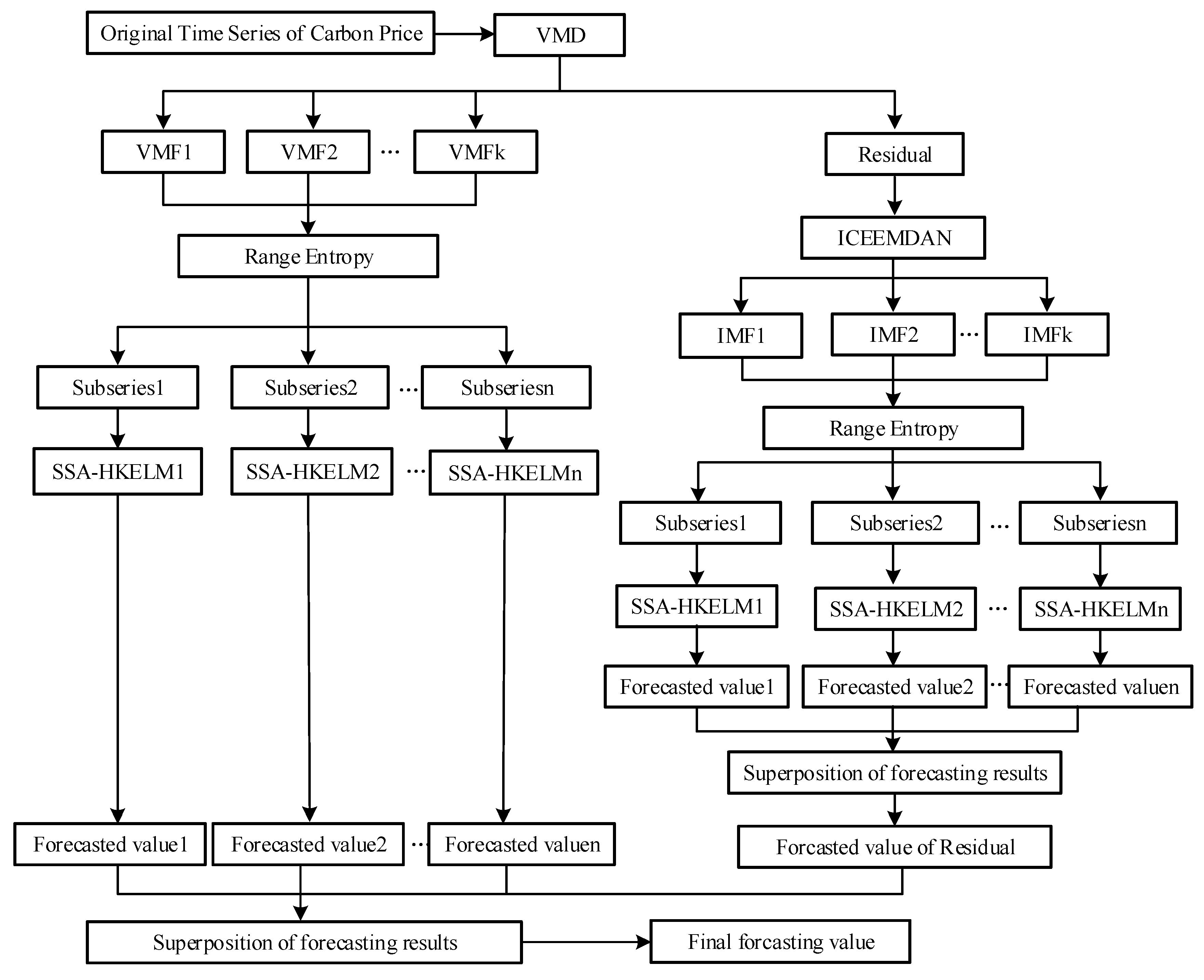
In view of the nonstationary, nonlinear, multi-frequency, and complex fluctuation-related characteristics of regional carbon prices in China, we construct a combined forecasting model based on secondary decomposition and the hybrid kernel-based extreme learning machine. The process diagram of the VMD-ICEEMDAN-RE-SSA-HKELM model is shown in Figure 1.

According to Figure 1, the steps of modeling are as follows:

(1)

VMD technology is used to decompose the original sequence of carbon prices to obtain each VMF, and the sum of the data is subtracted from the original time sequence of carbon prices to obtain the residual term of VMD.

(2)

Reconstruction and forecasting are carried out after VMD decomposition. We calculate RE of each VMF, and merge VMF components with lower entropies into a subseries. Each subseries is then forecasted using the SSA-HKELM model, and the results of each VMD-RE are obtained.

(3)

ICEEMDAN technology is used to decompose the residual term after VMD has been applied to the original sequence of carbon prices. Range entropy is introduced to measure the complexity of the signals of each IMF of the residual term, and IMF components with lower entropy values are merged into a new subseries. The SSA-HKELM model is then used to separately forecast each subseries of the residual term after applying ICEEMDAN-RE, and the results of the forecasts of each are further superimposed to obtain the final results of the residual term of the carbon price.

(4)

The results of the forecasting of each VMF and the residual term after the decomposition of the original sequence of carbon prices are superimposed to obtain the final forecasts of the carbon price.

4. Empirical Analysis of Price Forecasting of China’s Regional Carbon Markets

4.1. Sample Selection and Criteria for Evaluating Forecasts

We used regional market prices of carbon in China as the research object. Given that the trading volume of Hubei’s carbon market accounts for a large portion of that of the country, data on carbon pricing in this market from 3 January 2017 to 18 October 2021 were used. The sample size was 1158, and the data were obtained from the website of the Hubei Carbon Emission Trading Center (http://www.hbets.cn/list/13.html, accessed on 19 October 2021). All data on carbon prices and the models were processed in MATLAB 2019b. The routine statistical results of all sample data are shown in

Table 1. Descriptive statistics of the carbon price.

Market	Max	Min	Mean	Std	Skewness	Kurtosis
Hubei	53.85	11.26	25.74	8.21	0.10	2.46

.

The standard deviation of the transaction price in Hubei’s carbon market in Table 1 is 8.21, indicating that the data were relatively discrete. The difference between the maximum and minimum values was about 42 yuan/ton of carbon dioxide, indicating that the data were widely dispersed. Due to the impacts of policies, the macro-economy, and the market mechanism, the trading price in the carbon market was highly volatile.

Given the characteristics and limitations of the evaluation criteria in practice, it is difficult for any single evaluation index to comprehensively evaluate the advantages and disadvantages of the results of forecasting. To assess the proposed model, we used the root mean-squared error (RMSE), mean absolute error (MAE), and mean absolute percentage error (MAPE). The directional symmetry value (DS) was used to measure the capability of the proposed method to forecast the trend of the carbon price. In

Table 2. Evaluation criteria for the proposed model for forecasting the price of carbon.

	Index	Formula
Forecasting accuracy	RMSE	$\mathrm{RMSE}=\sqrt{\frac{1}{N}{\displaystyle \sum _{i=1}^N{(y_i-{\widehat{y}}_i)}^2}}$
	MAE	$\mathrm{MAE}=\frac{1}{N}{\displaystyle \sum _{i=1}^N\left|y_i-{\widehat{y}}_i\right|}$
	MAPE	$\mathrm{MAPE}=\frac{1}{N}{\displaystyle \sum _{i=1}^N\left|\frac{y_i-{\widehat{y}}_i}{y_i}\right|}$
Forecasting direction	DS	$\begin{array}{l}\mathrm{DS}=\frac{1}{N}{\displaystyle \sum _{i=1}^n{d}_i}\\ d_i=\left\{\begin{array}{l}1 , (y(t)-y(t-1))(\widehat{y}(t)-y(t-1))\ge 0\\ 0 , (y(t)-y(t-1))(\widehat{y}(t)-y(t-1))\le 0\end{array}\right.\end{array}$

, ${\widehat{y}}_i$ is the forecasted value of the carbon price, $y_i$ is the actual value, and N is the number of data items. The smaller RMSE, MAE, and MAPE were, and the larger DS was, the better the forecasts of the model.

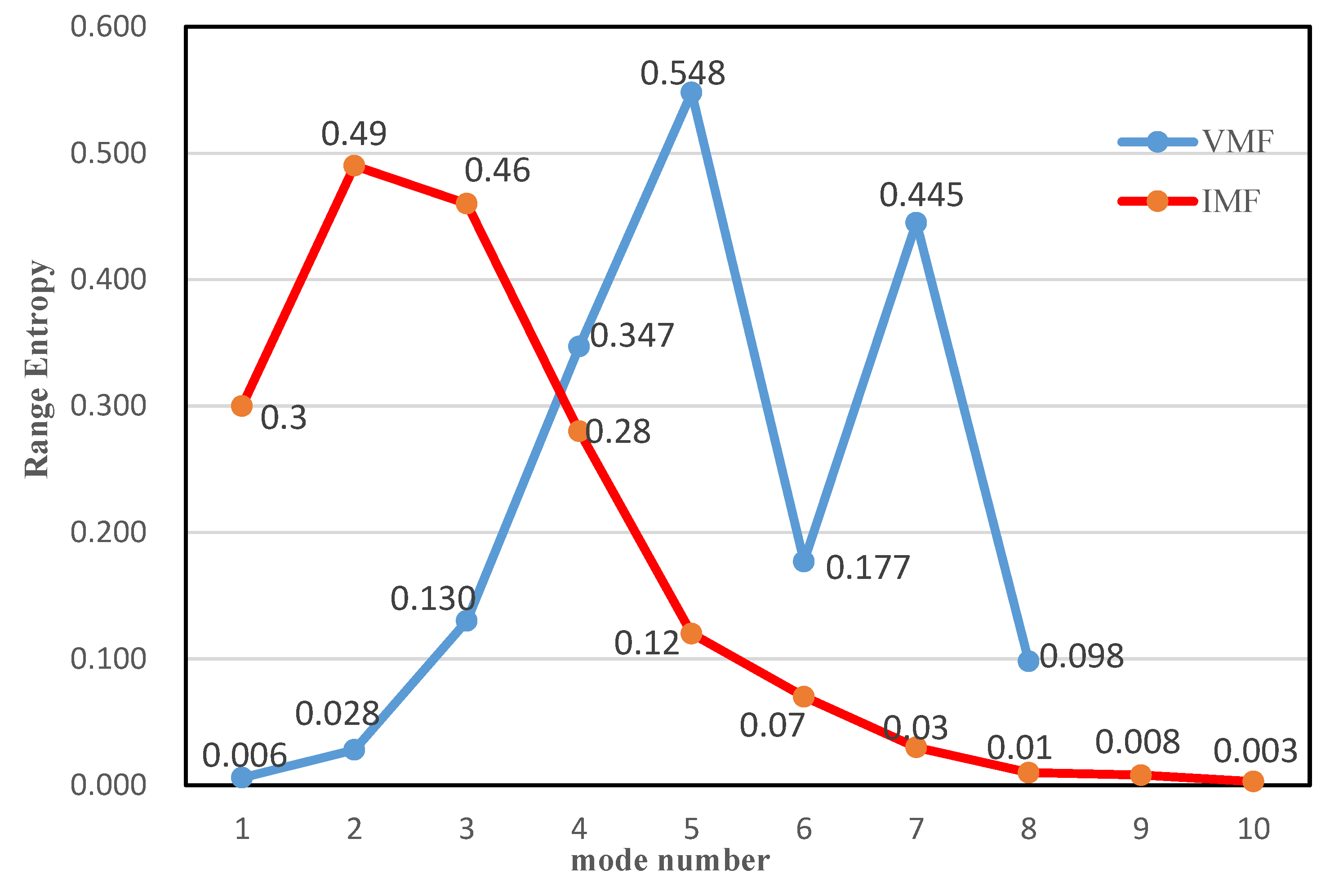
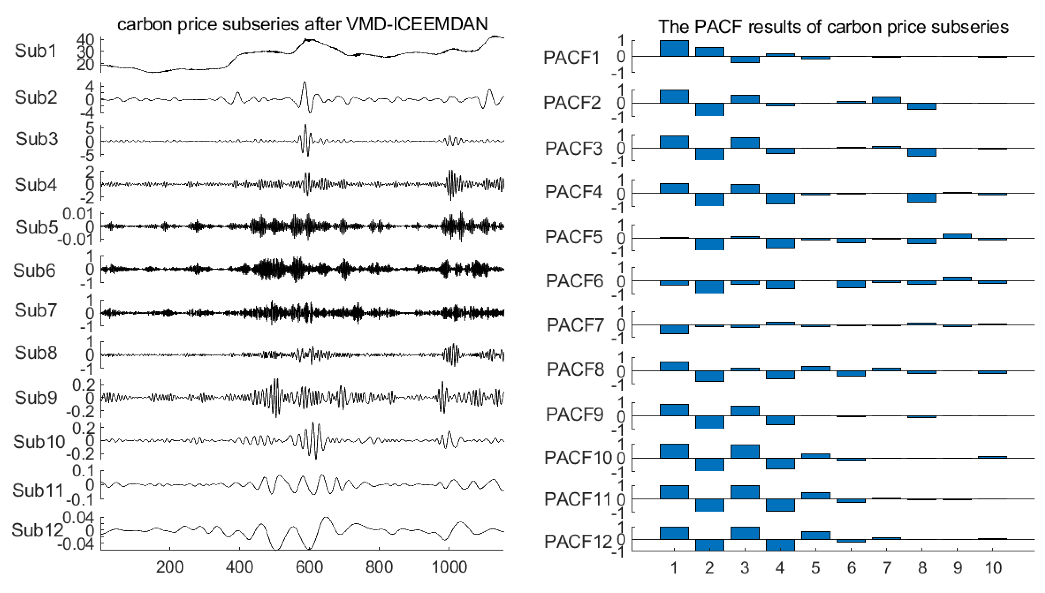
4.2. Analysis of the Decomposition and Reconstruction of the Market Price of Carbon

VMD was used to decompose the data on the time series of Hubei’s carbon prices in the sample period. The number K of components of the mode of decomposition of carbon prices needed to be set in advance. Different values of K lead to significant changes in the accuracy of carbon price forecasting. If the value of K is too small, the accuracy of decomposition decreases, and the complexity of the original sequence cannot be reduced. If the value of K is too large, it leads to excessive decomposition, and increases the amount of calculation and worsens the decomposition [45,46]. As ICEEMDAN can automatically decompose the data into an appropriate number of modes of the carbon price, we set the value of K by referring to the number of decompositions made by ICEEMDAN, which was eight. Specifically, eight VMF components were obtained. The results of the decomposition are shown in Figure 2. A residual term of the carbon price was obtained after VM, which was complex and fluctuated violently. It contained rich information on the carbon price. If this information is ignored in the forecasting model, the overall forecast is less accurate. Therefore, the residual term was subjected to ICEEMDAN, and the decomposed modes are shown in the upper-right part of Figure 2. The process of decomposition of VMD-ICEEMDAN is shown in Figure 2.

To reduce the cumulative error in the forecasted carbon prices, the RE algorithm was used to analyze the complexity of each VMF and IMF. The results are shown in Figure 3.

Figure 3 shows (1) an analysis of the range entropy of the results of VMD decomposition (VMFs) of the carbon price. The range entropies of VMF1, VMF2, and VMF8 were low, which indicates that their signals were not complex and had a long memory. They were merged into a new series. Because the range entropy values of VMF3–VMF7 were high with significant differences, the fluctuations in their signals were complicated and required separate forecasting. They were not reconstructed.

Figure 3 also shows (2) an analysis of the range entropy of the results of the decomposition of ICEEMDAN (IMFs) for the residual term of the carbon price. The range entropy values of IMF6–IMF10 were low, which indicates that their signals were not complex and had a long memory. IMF6–IMF10 were thus merged into a new subseries. The entropy values of IMF1 to IMF5 were high, which indicates that their signals were complex. They were not reconstructed but were forecasted separately.

Finally, 12 subseries were obtained as shown in

Table 3. Results of the reconstruction of the carbon price.

Original Carbon Price		Carbon Price Residual Sequence
Subseries	VMD Modes	Subseries	ICEEMDAN Modes
Sub1	VMF1, VMF2, VMF8	Sub7	IMF1
Sub2	VMF3	Sub8	IMF2
Sub3	VMF4	Sub9	IMF3
Sub4	VMF5	Sub10	IMF4
Sub5	VMF6	Sub11	IMF5
Sub6	VMF7	Sub12	IMF6, IMF7, IMF8, IMF9, IMF10

.

4.3. Partial Autocorrelation Test of Subseries of the Carbon Price

After the decomposition and reconstruction of the original carbon price, the input variables for the forecasting model of each subseries needed to be determined. The partial autocorrelation test was used to analyze the impact of historical data on each subseries of the carbon price at the 95% confidence level (Figure 4).

According to the results of the PACF test, each subseries of carbon prices was more regular after decomposition and reconstruction, and was affected by its own historical time series data. In general, recent historical data had a greater impact on the fluctuations in each subsequence of carbon prices than longer-term historical data. This shows that each reconstructed subsequence of carbon prices had a certain persistence, and its historical time series data contained important information for forecasting the price of carbon. Considering the results of the partial autocorrelation test of each subseries above, and given how large input variables in the HKELM forecasting model affected its accuracy and redundancy, the input variables of each forecasting model for the subseries of carbon prices determined in this paper are shown in

Table 4. Input variables of each forecasting model of the subseries of carbon prices.

Carbon Price Subseries	Input to Each HKELM Forecasting Model
Sub1	y(t − 1), y(t − 2), y(t − 3), y(t − 4), y(t − 5)
Sub2	y(t − 1), y(t − 2), y(t − 3), y(t − 4), y(t − 6)
Sub3	y(t − 1), y(t − 2), y(t − 3), y(t − 4)
Sub4	y(t − 1), y(t − 2), y(t − 3), y(t − 4), y(t − 5)
Sub5	y(t − 1), y(t − 2), y(t − 3), y(t − 4), y(t − 5), y(t − 6)
Sub6	y(t − 1), y(t − 2), y(t − 3), y(t − 4), y(t − 6)
Sub7, Sub8	y(t − 1), y(t − 2), y(t − 3), y(t − 4), y(t − 5)
Sub9	y(t − 1), y(t − 2), y(t − 3), y(t − 4)
Sub10, Sub11, Sub12	y(t − 1), y(t − 2), y(t − 3), y(t − 4), y(t − 5), y(t − 6)

.

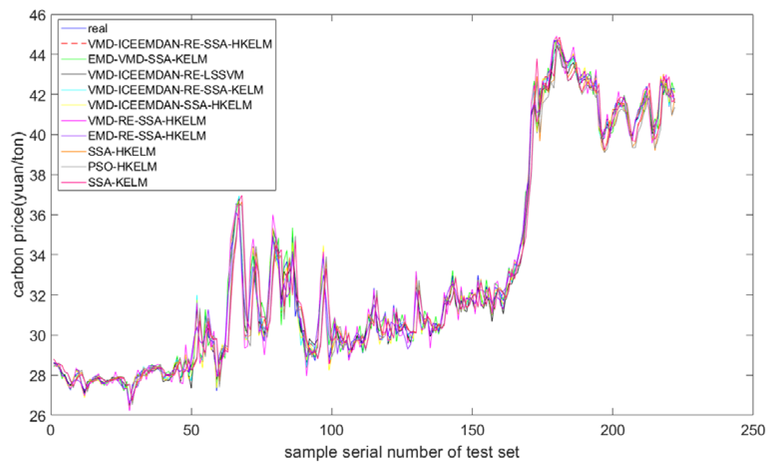
4.4. Analysis of the Forecasted Carbon Price

We used the data on the carbon price in the Hubei market from 3 January 2017 to 10 November 2020 as the training set, with a total of 928 groups of data being used to train the forecasting model. The data on carbon prices from 11 November 2020 to 18 October 2021 were used as the test set, with a total of 222 groups of data. To ensure the accuracy of the SSA-HKELM model, each subseries of the data on carbon prices needed to be normalized. We used the mapminmax function to normalize the input and output variables of each subseries to the interval [−1, 1]. Then, HKELM with the RBF kernel function and poly-kernel function was used to forecast each subseries of carbon prices. The optimal regularization parameters, parameters of the kernel function, and weights of the HKELM model were obtained by the SSA algorithm during model training. The results of the optimization of the parameters of HKELM for each subseries of carbon prices are shown in

Table 5. The results of the optimization of the parameters of HKELM for subseries of carbon prices.

Carbon Price Subseries	C	a	c	d	w
Sub1	804.2335	42.4727	406.3407	3	0.4152
Sub2	218.1153	20.4560	368.6420	2	0.7566
Sub3	285.8397	757.2005	753.7293	4	0.9172
Sub4	781.7228	490.4006	148.4659	1	0.1264
Sub5	281.9055	6.3548	273.3429	1	0.1022
Sub6	266.7218	100.3802	846.0002	1	0.7839
Sub7	641.6777	128.6927	0.0015	3	0.4092
Sub8	745.3274	424.0307	811.8651	1	0.4083
Sub9	0.0184	646.2312	332.7460	3	0.4833
Sub10	751.5801	363.3060	35.1337	3	0.0656
Sub11	260.3775	184.9134	115.1786	5	0.3729
Sub12	341.7896	590.9369	468.3994	4	0.7054

.

To investigate the forecasting performance of the model, 222 groups of data from 11 November 2020 to 18 October 2021 were used as the test set, and each subseries of carbon prices was tested by using the HKELM model optimized by SSA. The results of the forecasting of each subseries were linearly superimposed to obtain the final results of the predicted price of carbon. To verify the validity of the proposed model, it was compared with a reference group consisting of single forecasting models, such as SSA-KELM, PSO-HKELM, and SSA-HKELM; a combination of decomposition models, such as EMD-RE-SSA-HKELM and VMD-RE-SSA-HKELM; and combinations of secondary decomposition-based forecasting models, such as VMD-ICEEMDAN-SSA-HKELM, VMD-ICEEMDAN-RE-SSA-KELM, VMD-ICEEMDAN-RE-LSSVM, and EMD-VMD-SSA-KELM. The forecasting results of these models for the carbon price of Hubei are shown in Figure 5. They show that the proposed model achieved a high accuracy. This verifies its feasibility for predicting regional prices in the carbon markets in China.

Table 6. Comparison of the models in forecasting carbon prices in the Hubei market.

Models	RMSE	MAE	MAPE	DS
SSA-KELM	1.1760	0.8021	0.0243	0.5270
PSO-HKELM	1.2025	0.8598	0.0258	0.5450
SSA-HKELM	1.1697	0.8259	0.0250	0.5135
EMD-RE-SSA-HKELM	0.5257	0.3880	0.0120	0.8288
VMD-RE-SSA-HKELM	0.4181	0.3137	0.0096	0.8378
VMD-ICEEMDAN-SSA-HKELM	0.2578	0.1865	0.0058	0.8964
VMD-ICEEMDAN-RE-SSA-KELM	0.3092	0.2245	0.0069	0.8604
VMD-ICEEMDAN-RE-LSSVM	0.4086	0.2944	0.0089	0.8243
EMD-VMD-SSA-KELM	0.2869	0.2105	0.0064	0.8604
VMD-ICEEMDAN-RE-SSA-HKELM	0.2493 *	0.1796 *	0.0056 *	0.9054 *

Note: * indicates the best performance of each model.

gives a comparison of the models in forecasting carbon prices in the Hubei market.

Table 6 shows that KELM consisted of the RBF kernel; EMD-RE-SSA-HKELM represents a combined model with only EMD-based single decomposition; VMD-RE-SSA-HKELM represents a model that ignored the residual term of the carbon price after VMD; VMD-ICEEMDAN-SSA-HKELM represents a model that directly forecasted all modes of the secondary decomposition of the carbon price without reconstruction; VMD-ICEEMDAN-RE-SSA-KELM represents KELM with the RBF kernel to forecast each subseries of carbon prices after secondary decomposition and reconstruction; VMD-ICEEMDAN-RE-LSSVM represents the use of the LSSVM model to forecast each subseries of carbon prices after secondary decomposition and reconstruction; EMD-VMD-SSA-KELM is a combined model proposed in the literature [28]; and the combination of models proposed here is denoted by VMD-ICEEMDAN-RE-SSA-HKELM.

Table 6 shows that RMSE, MAE, and MAPE of the VMD-ICEEMDAN-RE-SSA-HKELM model were 0.2493, 0.1796, and 0.0056, respectively, and errors in it were smaller than in the other models in terms of the accuracy of forecasting the price of carbon. DS of the proposed model was the highest at 0.9054. This shows that the accuracy of forecasting of the carbon price and its trend by the proposed model, for the Hubei carbon market, were the highest of all single models and combined models considered.

A comparison of the results shows the following: (1) the proposed model (VMD-ICEEMDAN-RE-SSA-HKELM) was superior to VMD-ICEEMDAN-RE-SSA-KELM and VMD-ICEEMDAN-RE-LSSVM in terms of forecasting the price of carbon. HKELM was able to fully exploit the advantages of each kernel function to describe data on the fluctuations in the carbon price, which improved the forecasts of the subseries of carbon prices. (2) The forecasting performance of the combinations of models based on secondary decomposition was better than that of the single decomposition models. In comparison with the EMD, VMD, and VMD-ICEEMDAN models, ICEEMDAN better decomposed the residual term for the carbon price generated by VMD decomposition to significantly improve the forecasts. The VMD model was superior to the EMD model because it better decomposed the nonlinear and nonstationary carbon prices. For example, it solved the problem of modal aliasing in EMD and reduced the complexity of the series of carbon prices. Moreover, the residual term was decomposed by ICEEMDAN and incorporated into the model. This allowed for clarification of the trend of changes in and the frequency of carbon prices, and more comprehensively described the impact of all historical signals of the carbon prices on future trends. (3) The proposed model was superior to VMD-ICEEMDAN-SSA-HKELM because its reconstruction of the modes of the carbon prices based on range entropy reduced the cumulative error in the forecasted prices of carbon. (4) Among the single forecasting models, the SSA-HKELM model was better than the PSO-HKELM model because it was optimized by SSA to obtain the best parameters of regularization and the kernel and weights to avoid the subjective selection of these parameters. (5) Combinations of the models for forecasting the prices of carbon based on decomposition were superior to the single models. These included SSA-KELM, PSO-HKELM, and SSA-HKELM. This is because the original trend of the price of carbon was highly complex, such that a single model could not capture its nonlinearity and nonstationarity. (6) Forecasts of the proposed model were significantly better than those of EMD-VMD-SSA-KELM because the secondary decomposition technology of the former fully decomposed the carbon price.

In short, to forecast regional carbon prices in China based on secondary decomposition and HKELM, the combined model can completely decompose the complex series of market prices of carbon, and can significantly improve the accuracy of forecasting the price of carbon and its change trends.

4.5. Robustness

To further verify the robustness of the proposed model, we applied it to daily carbon prices of the Guangzhou Carbon Emission Exchange from 3 January 2017 to 18 October 2021. The results are shown in

Table 7. Comparison of the methods for forecasting the price of carbon in the Guangzhou market.

Models	RMSE	MAE	MAPE	DS
SSA-KELM	0.7380	0.5455	0.0146	0.4955
PSO-HKELM	0.7663	0.5453	0.0144	0.5631
SSA-HKELM	0.6191	0.4423	0.0118	0.5676
EMD-RE-SSA-HKELM	0.2927	0.2217	0.0059	0.8514
VMD-RE-SSA-HKELM	0.1352	0.1026	0.0027	0.9054
VMD-ICEEMDAN-SSA-HKELM	0.1057	0.0861	0.0023	0.8964
VMD-ICEEMDAN-RE-SSA-KELM	0.5669	0.4623	0.0118	0.6486
VMD-ICEEMDAN-RE-LSSVM	0.5218	0.4202	0.0108	0.6577
EMD-VMD-SSA-KELM	0.2884	0.2445	0.0065	0.7748
VMD-ICEEMDAN-RE-SSA-HKELM	0.0934 *	0.0706 *	0.0019 *	0.9189 *

Note: * indicates the best performance for all models.

. The relative values of the evaluation indicators did not change significantly from the results from Hubei, which shows that the proposed model for forecasting regional carbon prices in China is robust against varying markets.

5. Conclusions

Forecasting regional carbon prices is an important area of research on the financial market for carbon. Given that the traditional model used to predict regional prices in China is flawed, this paper proposed a forecasting model based on secondary decomposition and HKELM, and verified its performance on data on carbon prices from the Hubei market. The VMD method was used to decompose the original carbon price, ICEEMDAN was applied to decompose the residual term after VMD, and range entropy was used to reconstruct sequences with less complex signals than in the original series of data. The HKELM model was used to forecast each subseries, and PACF was used to select the input variables of each subseries of the model. The parameters of the HKELM model were optimized by SSA. Finally, forecasts of each subseries of carbon prices were superimposed to obtain the final forecast for the carbon price in the market. The results of comparative empirical analysis showed that the proposed model is superior to prevalent models in terms of forecasting the price of carbon.

The proposed model has the following advantages in comparison with prevalent models: (1) ICEEMDAN decomposes the complex residual term of the carbon price after VMD into several, more regular, subsequences to improve the accuracy of forecasting. Secondary decomposition is superior to the traditional model for secondary decomposition. (2) The use of HKELM to forecast each subseries of carbon prices helps determine the characteristics of fluctuation and the internal laws of different subseries of carbon prices to improve the accuracy and stability of the forecasts. (3) The complexity in the signals of each mode of carbon prices was analyzed using range entropy, and was used to reconstruct sequences with less complex signals to reduce the forecasting error and the workload required to forecast the price of carbon.

However, this study still has certain limitations. Firstly, although the proposed model is highly accurate, the trend of carbon prices in regional markets in China is determined by a number of complex factors, such as the supply and demand relationship in the carbon market; the prices of coal, crude oil, and natural gas; the macro-economic environment; climate change; and major public disasters. Such factors that are influential for the carbon market should be incorporated into the proposed model in future research in the area to improve forecasts of the carbon price. Secondly, this article only considered empirical research on the regional carbon price in China. Research on the carbon market price can be expanded and applied to the EU carbon price to verify the wide applicability of the model.

References

1. Sun, H.; Samuel, C.A.; Amissah, J.C.K.; Taghizadeh-Hesary, F.; Mensah, I.A. Non-linear nexus between CO2 emissions and economic growth: A comparison of OECD and B&R countries. Energy 2020, 212, 118637. [Google Scholar] [CrossRef]
2. Sun, H.; Edziah, B.K.; Sun, C.; Kporsu, A.K. Institutional quality and its spatial spillover effects on energy efficiency. Socio-Econ. Plan. Sci. 2021, 101023. [Google Scholar] [CrossRef]
3. Li, X.; Li, Z.; Su, C.; Umar, M.; Shao, X. Exploring the asymmetric impact of economic policy uncertainty on China’s carbon emissions trading market price: Do different types of uncertainty matter? Technol. Forecast. Soc. Chang. 2022, 178, 121601. [Google Scholar] [CrossRef]
4. Zheng, J.; Mi, Z.; Coffman, D.; Milcheva, S.; Shan, Y.; Guan, D.; Wang, S. Regional development and carbon emissions in China. Energy Econ. 2019, 81, 25–36. [Google Scholar] [CrossRef]
5. Huang, W.; Wang, Q.; Li, H.; Fan, H.; Qian, Y.; Klemeš, J. Review of recent progress of emission trading policy in China. J. Clean. Prod. 2022, 349, 131480. [Google Scholar] [CrossRef]
6. Liu, B.; Sun, Z.; Li, H. Can Carbon Trading Policies Promote Regional Green Innovation Efficiency? Empirical Data from Pilot Regions in China. Sustainability 2021, 13, 52891. [Google Scholar] [CrossRef]
7. Ren, C.; Lo, A.Y. Emission trading and carbon market performance in Shenzhen, China. Appl. Energy 2017, 193, 414–425. [Google Scholar] [CrossRef] [Green Version]
8. Zeng, S.; Nan, X.; Liu, C.; Chen, J. The response of the Beijing carbon emissions allowance price (BJC) to macroeconomic and energy price indices. Energy Policy 2017, 106, 111–121. [Google Scholar] [CrossRef]
9. Zhang, Y.; Liu, Z.; Xu, Y. Carbon price volatility: The case of China. PLoS ONE 2018, 13, e0205317. [Google Scholar] [CrossRef] [Green Version]
10. Han, M.; Ding, L.; Zhao, X.; Kang, W. Forecasting carbon prices in the Shenzhen market, China: The role of mixed-frequency factors. Energy 2019, 171, 69–76. [Google Scholar] [CrossRef]
11. Huang, Y.; Hu, J.; Liu, H.; Liu, S. Research on price forecasting method of China’s carbon trading market based on PSO-RBF algorithm. Syst. Sci. Control. Eng. 2019, 7, 40–47. [Google Scholar] [CrossRef]
12. Xie, Q.; Hao, J.; Li, J.; Zheng, X. Carbon price prediction considering climate change: A text-based framework. Econ. Anal. Policy 2022, 74, 382–401. [Google Scholar] [CrossRef]
13. Liu, J.; Wang, P.; Chen, H.; Zhu, J. A combination forecasting model based on hybrid interval multi-scale decomposition: Application to interval-valued carbon price forecasting. Expert Syst. Appl. 2022, 191, 116267. [Google Scholar] [CrossRef]
14. Fan, J.; Todorova, N. Dynamics of China’s carbon prices in the pilot trading phase. Appl. Energy 2017, 208, 1452–1467. [Google Scholar] [CrossRef] [Green Version]
15. Zhu, B. A novel multiscale ensemble carbon price prediction model integrating empirical mode decomposition, genetic algorithm and artificial neural network. Energies 2012, 5, 355–370. [Google Scholar] [CrossRef]
16. Li, W.; Lu, C. The research on setting a unified interval of carbon price benchmark in the national carbon trading market of China. Appl. Energy 2015, 155, 728–739. [Google Scholar] [CrossRef]
17. Yao, Y.; Lv, J.; Zhang, C. Price formation mechanism and price forecast of Hubei carbon market. Stat. Decis. 2017, 19, 166–169. [Google Scholar]
18. Zhou, J.; Yu, X.; Yuan, X. Predicting the carbon price sequence in the Shenzhen Emissions Exchange using a multiscale ensemble forecasting model based on ensemble empirical mode decomposition. Energies 2018, 11, 1907. [Google Scholar] [CrossRef] [Green Version]
19. Wu, Q.; Liu, Z. Forecasting the carbon price sequence in the Hubei emissions exchange using a hybrid model based on ensemble empirical mode decomposition. Energy Sci. Eng. 2020, 8, 2708–2721. [Google Scholar] [CrossRef] [Green Version]
20. Lu, H.; Ma, X.; Huang, K.; Azimi, M. Carbon trading volume and price forecasting in China using multiple machine learning models. J. Clean. Prod. 2020, 249, 119386. [Google Scholar] [CrossRef]
21. Jiang, P.; Liu, Z. Variable weights combined model based on multi-objective optimization for short-term wind speed forecasting. Appl. Soft. Comput. 2019, 82, 105587. [Google Scholar] [CrossRef]
22. Hao, Y.; Tian, C.; Wu, C. Modelling of carbon price in two real carbon trading markets. J. Clean. Prod. 2020, 244, 118556. [Google Scholar] [CrossRef]
23. Zhou, J.; Chen, D. Carbon Price forecasting based on improved CEEMDAN and extreme learning machine optimized by sparrow search algorithm. Sustainability 2021, 13, 94896. [Google Scholar] [CrossRef]
24. Sun, G.; Chen, T.; Wei, Z.; Sun, Y.; Zang, H.; Chen, S. A carbon price forecasting model based on variational mode decomposition and spiking neural networks. Energies 2016, 9, 54. [Google Scholar] [CrossRef] [Green Version]
25. Chai, S.; Zhang, Z.; Zhang, Z. Carbon price prediction for China’s ETS pilots using variational mode decomposition and optimized extreme learning machine. Ann. Oper. Res. 2021. [Google Scholar] [CrossRef]
26. Sun, S.; Jin, F.; Li, H.; Li, Y. A new hybrid optimization ensemble learning approach for carbon price forecasting. Appl. Math. Model. 2021, 97, 182–205. [Google Scholar] [CrossRef]
27. Sun, W.; Huang, C. A carbon price prediction model based on secondary decomposition algorithm and optimized back propagation neural network. J. Clean. Prod. 2020, 243, 118671. [Google Scholar] [CrossRef]
28. Zhou, J.; Wang, S. A carbon price prediction model based on the secondary decomposition algorithm and influencing factors. Energies 2021, 14, 1328. [Google Scholar] [CrossRef]
29. Zhou, J.; Wang, Q. Forecasting carbon price with secondary decomposition algorithm and optimized extreme learning machine. Sustainability 2021, 13, 58413. [Google Scholar] [CrossRef]
30. Dragomiretskiy, K.; Zosso, D. Variational mode decomposition. IEEE Trans. Signal Process. 2014, 62, 531–544. [Google Scholar] [CrossRef]
31. Li, H.; Jin, F.; Sun, S.; Li, Y. A new secondary decomposition ensemble learning approach for carbon price forecasting. Knowl.-Based Syst. 2021, 214, 106686. [Google Scholar] [CrossRef]
32. Colominas, M.A.; Schlotthauer, G.; Torres, M.E. Improved complete ensemble EMD: A suitable tool for biomedical signal processing. Biomed. Signal Process. Control. 2014, 14, 19–29. [Google Scholar] [CrossRef]
33. Jia, S.; Ma, B.; Guo, W.; Li, Z.S. A sample entropy based prognostics method for lithium-ion batteries using relevance vector machine. J. Manuf. Syst. 2021, 61, 773–781. [Google Scholar] [CrossRef]
34. Ru, Y.; Li, J.; Chen, H.; Li, J. Epilepsy Detection Based on Variational Mode Decomposition and Improved Sample Entropy. Comput. Intell. Neurosci. 2022, 2022, 6180441. [Google Scholar] [CrossRef]
35. Omidvarnia, A.; Mesbah, M.; Pedersen, M.; Jackson, G. Range entropy: A bridge between signal complexity and self-similarity. Entropy 2018, 20, 962. [Google Scholar] [CrossRef] [Green Version]
36. Huang, G.; Zhou, H.; Ding, X.; Zhang, R. Extreme learning machine for regression and multiclass classification. IEEE Trans. Syst. Man Cybern. Part B-Cybern. 2012, 42, 513–529. [Google Scholar] [CrossRef] [Green Version]
37. Zhang, T.; Tang, Z.; Wu, J.; Du, X.; Chen, K. Multi-step-ahead crude oil price forecasting based on two-layer decomposition technique and extreme learning machine optimized by the particle swarm optimization algorithm. Energy 2021, 229, 120797. [Google Scholar] [CrossRef]
38. Qi, X.; Li, K.; Yu, X.; Zhang, Z.; Lou, J. Transformer top oil temperature interval prediction based on kernel extreme learning machine and bootstrap method. Proc. CSEE 2017, 37, 5821–5828. [Google Scholar]
39. Zhou, C.; Yin, K.; Cao, Y.; Intrieri, E.; Ahmed, B.; Catani, F. Displacement prediction of step-like landslide by applying a novel kernel extreme learning machine method. Landslides 2018, 15, 2211–2225. [Google Scholar] [CrossRef] [Green Version]
40. Hou, Z.; Lao, W.; Wang, Y.; Lu, W. Hybrid homotopy-PSO global searching approach with multi-kernel extreme learning machine for efficient source identification of DNAPL-polluted aquifer. Comput. Geosci. 2021, 155, 104837. [Google Scholar] [CrossRef]
41. Li, T.; Qian, Z.; He, T. Short-Term Load Forecasting with Improved CEEMDAN and GWO-Based Multiple Kernel ELM. Complexity 2020, 2020, 1209547. [Google Scholar] [CrossRef]
42. Lv, L.; Wang, W.; Zhang, Z.; Liu, X. A novel intrusion detection system based on an optimal hybrid kernel extreme learning machine. Knowl.-Based Syst. 2020, 195, 105648. [Google Scholar] [CrossRef]
43. Xue, J.K.; Shen, B. A novel swarm intelligence optimization approach: Sparrow search algorithm. Syst. Sci. Control. Eng. 2020, 8, 22–34. [Google Scholar] [CrossRef]
44. Xin, J.; Chen, J.; Li, C.; Lu, R.; Li, X.; Wang, C.; Zhu, H.; He, R. Deformation characterization of oil and gas pipeline by ACM technique based on SSA-BP neural network model. Measurement 2022, 189, 110654. [Google Scholar] [CrossRef]
45. Niu, M.; Hu, Y.; Sun, S.; Liu, Y. A novel hybrid decomposition-ensemble model based on VMD and HGWO for container throughput forecasting. Appl. Math. Model. 2018, 57, 163–178. [Google Scholar] [CrossRef]
46. Zhang, Y.; Pan, G.; Chen, B.; Han, J.; Zhao, Y.; Zhang, C. Short-term wind speed prediction model based on GA-ANN improved by VMD. Renew. Energy 2020, 156, 1373–1388. [Google Scholar] [CrossRef]
Figure 1. Flowchart of the proposed model for forecasting the price of carbon, VMD-ICEEMDAN-RE-SSA-HKELM.
Energies 15 03562 g001
Figure 2. Secondary decomposition of the carbon price using VMD-ICEEMDAN.
Energies 15 03562 g002
Figure 3. Range entropy analysis of the decomposition of the carbon price.
Energies 15 03562 g003
Figure 4. Reconstructed results of the carbon price and the results of their PACF test.
Energies 15 03562 g004
Figure 5. Results of the predicted carbon prices in the Hubei market.
Energies 15 03562 g005