Study of Pressure Retarded Osmosis Process in Hollow Fiber Membrane: Cylindrical Model for Description of Energy Production

Abstract

A new mathematical model was developed to predict the cylindrical effect of the membrane performance in the pressure retarded osmosis process. The cylindrical membrane transport layers (the draw side boundary and the porous membrane) were divided into very thin sublayers with constant mass transport parameters, among others with a constant radius in every sublayer. The obtained second-order differential mass balance equations were solved analytically, with constant parameters written for every sublayer. The algebraic equation system involving 2N equations was then solved for the determinant solution. It was shown that the membrane properties, water permeability (A), salt permeability (B), structural parameter (S) and the operating conditions (inlet draw side solute concentration and draw side mass transfer coefficient) affect the water flux strongly, and thus the membrane performance, due to the cylindrical effect caused by the variable surface and volume of the sublayers. This effect significantly depends on the lumen radius. The lower radius means a larger change in the internal surface/volume of sublayers with ΔR thickness. The predicted results correspond to that of the flat-sheet membrane layer at r_o = 10,000 μm. At the end of this manuscript, the calculated mass transfer rates were compared to those measured. It was stated that the curvature effect in using a capillary membrane must not be left out of consideration when applying hollow fiber membrane modules due to their relatively low lumen radius. The presented model provides more precise prediction of the performance in the case of hollow fiber membranes.

1. Introduction

The basic idea of energy production by osmotically driven membrane process, namely by pressure retarded osmosis (PRO), for the generation of so called “blue energy”, has been known for a long time [1,2]. The starting equation for the description of the solute and water flux, and consequently the harvestable energy, was developed by Lee et al. [2], which takes into account the effect of the thin dense active layer and the porous support layer. Later, McCutcheon and Elimelech [3] extended this model, taking into account the mass transport resistance of the fluid boundary layer of the higher solute concentration side of the asymmetric membrane. Nagy [4], then Bui et al. [5], extended this model for all the four mass transport layers, namely active and the support membrane layers, and the two external boundary layers of the higher salinity draw and the lower salinity feed laminar transport layers. During the last decades, several papers have studied the transport description [6,7,8,9], membrane characterization [10,11], possibility of energy generation applying seawater–river water pair [12,13], and the effect of non-ideality [14,15]. Books [16,17] provide comprehensive reviews for technologies and applications of processes, as PRO, reverse electrodialysis and capacitive mixing, using the salinity gradient for energy production.

The experimental and theoretical results, cited above, were carried out for a flat-sheet asymmetric membrane. With wide spreading of the hollow fiber and capillary membrane modules, in both their industrial and laboratory applications, the model description of the transport through cylindrical membranes emerged. Several papers also applied hollow fiber membrane modules for PRO systems [16,17,18,19,20]. Sivertsen et al. [21] developed a mathematical model for the cylindrical membrane, taking all four mass transfer resistances into account. In their model, the volumetric flux is related to that at the membrane surface, thus, J_w,ror_o = J_wr, i.e., at r = r J_w = J_w,ror_o/r. The mass transfer rate was defined as J = −DdC/dr. Thus, the solute transfer rate was defined for every transport layer. Accordingly, the authors obtained a model with five unknown parameters, C_m, C_s, C_sp, J_w and J_s, as well as five implicit equations with five known transport parameters, which were solved by “guessing a water flux and iterated until the anticipated water flux” corresponds to the equations given for the individual transport layers [21]. The question might be whether there is only one solution of a problem with five variables and when there is more, than which one is the real one. Cheng et al. [22] studied the forward osmosis-pressure retarded osmosis hybrid process using hollow fiber membrane modules. They described the mass transport using a cylindrical coordinate, as it was applied by Siversten et al. [21]. They have taken into account that the water flux continuously varies due to the membrane radius. In order to get the water flux by easy integration of the transfer rate equations, “a concept of linear water flux and linear reverse salt flux has to be defined”, namely ξ_w = J_w2π(r), and ξ_s = J_s2π(r) [9,22]. Then the known water flux expressions defined for flat-sheet were modified with ξ_w (and ξ_s). These modified expressions were used to calculate the water and solute fluxes, taking into account the cylindrical effect. After predicting the water flux, the structural parameter was determined without considering the effect of the external mass transfer resistances [22].

This paper aims to discuss the cylindrical effect on mass transport through the hollow fiber membrane module in the case of pressure retarded osmosis or forward osmosis processes. This paper presents a cylindrical model, which defines the inlet mass transfer rate for every important mass transfer layer, namely for the active and support membrane layers, and the boundary layer of a high salinity draw solution. The model serves as an analytical approach solution of the mass transport, dividing the transport layer into very thin sub-layers assuming that the variable mass transport parameters and the radius are constant in every single sub-layer. The algebraic equation systems, obtained after the analytical solution of the sub-layers’ differential equations, can be solved by conventional solution methodology, used for the determinant. Knowing the inlet transport rates for every transport layer, in closed form, the overall mass transfer rate can easily be expressed. Similar to the flat-sheet solution, the water flux can be obtained by iteration due to the implicit expressions, regarding the water flux. In the end, the model data are validated by measured data

2. Materials and Methods

The main points are to develop a new mathematical model, which describes the mass transport through the asymmetric capillary membrane layer for hydraulic and/or osmotic pressure-driven, PRO or RO, membrane processes. The essence of this model is that every single transport layer has diffusive plus convective flow, thus the draw side boundary layer and the porous support membrane layer are divided into very thin transport layers (a number for it, N, in this case, was chosen to be 1000; see details in Section 3) with constant mass transport parameters, among others, the membrane radius as well. The dense active membrane layer involves only diffusive flow, its concentration gradient is linear, independently of the radius, due to its very thin thickness. The second order differential expression, given for every sub-layer, with constant parameters, can be solved analytically. Expressing the integration parameters by suitable boundary conditions, one obtains 2N number algebraic equations, an equation system which can then be solved by conventional mathematical methods applying for a determinant solution [23,24].

The theoretical results are used to predict the effect of the cylindrical coordinate on the water flux as well as on the power density. The figures show how strongly the membrane radius can affect the water flux, and membrane performance. The mathematical model data are validated measured data taken from the literature in the last sub-sections.

3. Theory

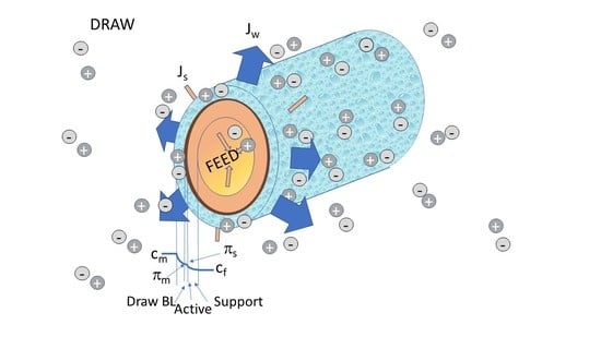
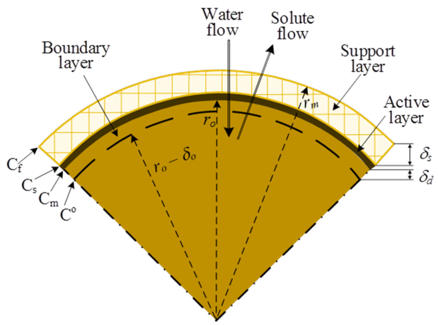
The capillary hollow fiber membrane is the most often applied membrane module in the separation industry, due to its very advantageous surface/volume ratio. The very thin lumen radius and membrane thickness can provide favorable mass transport conditions and separation conditions. The schematic illustration of a capillary, with the important notations, is given in Figure 1. The component transport can take place either from the porous or the selective sides of a cylindrical membrane, depending on the location of the immobilized biocatalyst. The differential mass balance equation in a steady-state condition, assuming diffusive and convective transport and variable mass transport parameters [D(C,r), v_max (r)] is as [24,25]:

$$D\left(C,r\right)\left(\frac{d^{2}C}{d{r}^2}+\frac{1}{r}\frac{dC}{dr}\right)+v\frac{dC}{dr}=0$$

(1)

with

$$P{e}_o=\frac{v_o{r}_o}{D\left(R\right)}$$

(2)

Rewriting Equation (1) in general dimensionless form, one can get as (R = r/r_o):

$$\frac{d^{2}C}{d{R}^2}+\frac{1+P{e}_o}{R}\frac{dC}{dR}=0$$

(3)

The solution of the above differential equation by constant parameters can analytically be solved by Bessel function [26]. We have looked for such an approach solution, which can be used in case of variable mass transfer coefficient (e.g., variable diffusion coefficient), and the transport properties, e.g., the inlet overall mass transfer rate, and the concentration distribution, can be expressed in closed, explicit mathematical expressions. For the approach solution, the following simplification was applied: the membrane layer was divided into N (during our simulation its value was chosen to be 1000) very thin sub-layers, with constant values of the variable diffusion coefficient, with the R value also considered as constant in every single sub-layer. The average radius, ${\overline{R}}_i$ was used (e.g., its algebraic mean value is considered in every sub-layer, [${\overline{R}}_i=1+\left(i-0.5\right)\Delta R$; $\Delta R=\delta /(N{r}_o)$; r_o is the lumen radius of the cylindrical membrane, m]). The obtained differential equation, with constant parameters, for the ith sub-layer (i = 1, …, N) is as:

$$\frac{d^{2}C}{d{R}^2}+\frac{1+P{e}_o}{{\overline{R}}_i}\frac{dC}{dR}=0$$

(4)

The general solution of Equation (4) is as:

$$C=T_i\exp \left(-\frac{1+P{e}_o}{{\overline{R}}_i}R\right)+S_i$$

(5)

Values of T_i and S_i represent the constants of the general solution. Suitable internal and outer boundary conditions should determine their values. The internal boundary conditions, written for every single sub-layer will be as follows:

For the internal concentrations, they are equal to each other at both sides of the inlet interface (see Appendix A):

$$T_i{e}^{-{\mathsf{\Theta }}_i{R}_i}+S_i=T_{i+1}{e}^{-{\mathsf{\Theta }}_{i+1}{R}_i}+S_{i+1},\left(i=1,\dots ,N-1\right)$$

(6)

where

$${\mathsf{\Theta }}_i=\frac{1+P{e}_o}{{\overline{R}}_i}$$

(7)

The mass transfer rate in the presence of diffusive plus convective flows can be expressed as (R_i = 1 + iΔR; ΔR = δ_d/(Nr_o) for the liquid boundary layer on the draw side; ΔR = δ_s/(Nr_o) for the membrane support layer:

$$J_i=-\frac{D}{r_o}{\left.\frac{dC}{dR}\right|}_{R=R_i}-\frac{D}{r_o}{\left.\frac{P{e}_o}{{\overline{R}}_i}C\right|}_{R=R_i},\left(i=1,\dots ,N-1\right)$$

(8)

For the internal mass transfer rates, considering the equality of them at the two sides of the interface:

$${\overline{R}}_i\left(T_i\frac{e^{-{\mathsf{\Theta }}_{i}R}i}{{\overline{R}}_i}-S_i\frac{P{e}_o}{{\overline{R}}_i}\right)={\overline{R}}_{i+1}\left(T_{i+1}\frac{e^{-{\mathsf{\Theta }}_{i+1}{R}_i}}{{\overline{R}}_{i+1}}-S_i\frac{P{e}_o}{{\overline{R}}_{i+1}}\right),\left(i=1,\dots ,N-1\right)$$

(9)

While the inlet and outlet boundary conditions are, respectively (for o, m, s, sp see Figure 1):

$$C_j=T_1{e}^{-{\mathsf{\Theta }}_1}+S_1,j=o,m$$

(10)

and (R_m = 1 + NΔR)

$$C_k=T_N{e}^{-\mathsf{\Theta }{R}_m}+S_N,k=s,sp$$

(11)

It is important to note that this mathematical model will be applied for two mass transport layers, namely for the draw side boundary layer (its inlet and outlet concentrations are C^o and C_m (see Figure 1), respectively) and the membrane porous support layer (its inlet and outlet concentrations are C_s and C_f, respectively). The effect of the fluid boundary layer of the feed side is generally not higher than 5% [24], thus its effect on the overall mass transfer resistance is neglected here for the sake of simplicity. Applying the internal (Equations (7) and (9)) and the external (Equations (10) and (11)) boundary conditions, one can get three N × N dimensional determinants (see e.g., [24]). These determinants are used to determine the T_i and S_i (i = 1 − N) values, applying the known determinant’s laws [23]. The solution of this special problem (not shown here in detail; several examples are shown in Nagy’s book [24] on it: see e.g., pp. 144–150, 177–183 or 279–282, where the same calculation methodology is used) is, e.g., for the boundary layer, as follows (δ_d is the thickness of the boundary layer):

$$T_1=\left(C_j{\displaystyle \prod _{i=1}^{i=N}\frac{A_{T,i}}{A_{O,i}}-}\frac{C_k}{{\displaystyle \prod _{i=1}^{i=N-1}{A}_{O,i}}}\right)\frac{1}{e^{-{\mathsf{\Theta }}_1{r}_o/\left(r_o-{\delta }_d\right)}}$$

(12)

It is important to note that the multiplication factor after the parentheses will be $e^{-{\mathsf{\Theta }}_1}$, since the value of the local coordinate is unity in case of the membrane support layer. However, it is obvious the values of Θ are different in the two layers due to the different values of the local coordinate and other parameters, which are dependent on the R value. The value of S₁ is as:

$$S_1=\left(C_j{\displaystyle \prod _{i=1}^{i=N}\frac{A_{s,i}}{A_{O,i}}-}\frac{C_k}{{\displaystyle \prod _{i=1}^{i=N}{A}_{O,i}}}\right)$$

(13)

The values of other parameters are as:

$$A_{O,1}=1-e^{{\mathsf{\Theta }}_1\Delta R},{\mathrm{ B}}_{O,1}=-\left(P{e}_o+e^{-{\mathsf{\Theta }}_1\Delta R}\right)$$

(14)

$$A_{T,1}=1,{\mathrm{ B}}_{T,1}=-P{e}_o$$

(15)

$$A_{S,1}=-e^{{\mathsf{\Theta }}_1\Delta R},{\mathrm{ B}}_{S,1}=-e^{{\mathsf{\Theta }}_1\Delta R}$$

(16)

as well as

$$A_{j,i}=\frac{\left(1-e^{-{\mathsf{\Theta }}_i\Delta R}\right)}{1+P{e}_o}\left(\frac{B_{j,i-1}}{A_{j,i-1}}\right)-e^{{\mathsf{\Theta }}_i\Delta R}$$

(17)

and

$$B_{j,i}=\frac{\left(-P{e}_o-e^{-{\mathsf{\Theta }}_i\Delta R}\right)}{1+P{e}_o}\left(\frac{B_{j,i-1}}{A_{j,i-1}}\right)-e^{{\mathsf{\Theta }}_i\Delta R},j=O,T,S;i=2,\dots ,N$$

(18)

The values of T₁ and S₁ (note the S₁ value can also be predicted by Equation (10) in the knowledge of the value of T₁) can be calculated by applying Equations (14)–(18). Then, the inlet mass transfer rate of both the transport resistance can be calculated, on the basis of Equation (9), as shown below.

The above expressions can be applied independently of the two transport layers: the liquid boundary layer and the porous support layer. The very thin active layer involves diffusion flow only. The mass transport inside this layer is independent of the curvature of the space.

3.1. Expressing the Mass Transfer Rates

In the knowledge of T₁ and S₁, the individual mass transfer rates and the overall mass transfer rate can easily be defined. Then the curvature effect on the overall inlet mass transfer rates and thus its effect on the membrane performance can be discussed. Next, the mass transfer rate expressions will be given and discussed.

The Inlet Mass Transfer Rates of the Single Mass Transport Layers

The mass transfer rate is the sum of the diffusive and convective flows. Let us to look at first the inlet mass transfer rate for the draw side liquid boundary layer as an example, taking into account Equations (3) and (8). Accordingly, the mass transfer rate will be as:

$$J_s=\frac{D}{r_o}\left(\frac{1+P{e}_o}{{\overline{R}}_i}\right)T_i{e}^{-{\mathsf{\Theta }}_i{R}_i}-\frac{P{e}_i}{r_o}\left(T_i{e}^{-{\mathsf{\Theta }}_i{R}_i}+S_i\right)$$

(19)

Accordingly, the solute transfer rate is as:

$$J_s=\frac{D}{r_o}\left(\frac{1}{{\overline{R}}_i}{T}_i{e}^{-{\mathsf{\Theta }}_i{R}_i}-\frac{P{e}_i}{{\overline{R}}_i}{S}_i\right)$$

(20)

Thus, the draw side inlet mass transfer rate, taking into account Equations (12) and (13), will be as (C^o is the bulk concentration; C_m is the concentration on the selective layer):

$$J_s=\frac{D}{r_o}\left({\mathsf{\psi }}_d{C}^o-{\mathsf{\kappa }}_d{C}_m\right)$$

(21)

where

$${\mathsf{\psi }}_d={\displaystyle \prod _{i=1}^{i=N}\frac{A_{T,i}}{A_{O,i}}}-\frac{P{e}_o}{{\overline{R}}_1}{\displaystyle \prod _{i=1}^{i=N}\frac{A_{S,i}}{A_{O,i}}}$$

(22)

and

$${\mathsf{\kappa }}_d=\frac{P{e}_o}{{\overline{R}}_1}\left(\frac{1}{e^{-{\mathsf{\Theta }}_1}{\displaystyle \prod _{i=1}^{i=N-1}{A}_{O,i}}}-\frac{1}{{\displaystyle \prod _{i=1}^{i=N}{A}_{O,i}}}\right)$$

(23)

The inlet mass transfer rate for the membrane support layer can be similarly given to Equation (21). The form of the parameters ${\mathsf{\psi }}_s$ and ${\mathsf{\kappa }}_s$ is the same as Equations (22) and (23), respectively. Thus, now, the overall mass transfer rate can relatively easily be expressed as it is shown in Section 3.2.

3.2. The Overall Inlet Cylindrical Mass Transfer Rate

As it was mentioned, three transport layers, namely the fluid boundary layer, the active membrane layer and the porous support layer, should be taken into account for the expression of the overall mass transfer rate, J_ov. Equations (12)–(23) should calculate the boundary and the membrane support layer, taking into account that all parameters in these expressions, having subscript, are different in the two transport layers due to the fact that the change in the R_i and ${\overline{R}}_i$ values is different. Accordingly, the three inlet mass transfer rates, i.e., those for the liquid boundary layer, of the active membrane layer and for the porous support layer, will be, respectively, as:

$$J_s=\frac{D}{r_o}\frac{r_o}{r_o-{\delta }_s}\left({\mathsf{\psi }}_d{C}^o-{\mathsf{\kappa }}_d{C}_m\right),\hspace{1em}1-\frac{{\delta }_d}{r_o}\le R_i\le 1,\hspace{1em}{\overline{R}}_1,\dots ,{\overline{R}}_N$$

(24)

where

$${\mathsf{\psi }}_d={〈{\displaystyle \prod _{i=1}^{i=N}\frac{A_{T,i}}{A_{O,i}}}-\frac{P{e}_o}{{\overline{R}}_1}{\displaystyle \prod _{i=1}^{i=N}\frac{A_{S,i}}{A_{O,i}}}〉}_d$$

(25)

and

$${\mathsf{\kappa }}_d={\langle \frac{P{e}_o}{{\overline{R}}_1}\left(\frac{1}{e^{-{\mathsf{\Theta }}_1{r}_o/\left(r_o-{\delta }_s\right)}{\displaystyle \prod _{i=1}^{i=N-1}{A}_{O,i}}}-\frac{1}{{\displaystyle \prod _{i=1}^{i=N}{A}_{O,i}}}\right)\rangle }_d$$

(26)

For the determination of the overall mass transfer rate, the value of the mass transfer rate of the boundary layer should be defined for its outlet surface (R = 1), since the mass transfer rate of the other two transport layers are also related to this surface (the thickness of the selective layer is neglected). That is why the J_s value in Equation (24) is multiplied by a factor of r_o/(r_o − δ_s).

For the membrane active layer (C_s means the concentration of the surface of the selective and support layer i):

$$J_s=-B\left(C_m-C_s\right)$$

(27)

as well as for the membrane support layer (R_i = 1 + iΔR; ΔR = δ_s/(Nr_o); ${\overline{R}}_i=R_{i-1}+\Delta R/2$; ${\overline{R}}_1\simeq 1+\Delta R/2$; the thickness of the active layer can be negligible; C_f is the concentration of the feed side):

$$J_s=\frac{D}{r_o}\left({\mathsf{\psi }}_s{C}_s-{\mathsf{\kappa }}_s{C}_f\right),\hspace{1em}1\le R_i\le 1+\frac{{\delta }_s}{r_o},\hspace{1em}{\overline{R}}_1,\dots ,{\overline{R}}_N$$

(28)

where

$${\mathsf{\psi }}_s={〈{\displaystyle \prod _{i=1}^{i=N}\frac{A_{T,i}}{A_{O,i}}}-\frac{P{e}_o}{{\overline{R}}_1}{\displaystyle \prod _{i=1}^{i=N}\frac{A_{S,i}}{A_{O,i}}}〉}_s$$

(29)

and

$${\mathsf{\kappa }}_s={\langle \frac{P{e}_o}{{\overline{R}}_1}\left(\frac{1}{e^{-{\mathsf{\Theta }}_1}{\displaystyle \prod _{i=1}^{i=N-1}{A}_{O,i}}}-\frac{1}{{\displaystyle \prod _{i=1}^{i=N}{A}_{O,i}}}\right)\rangle }_s$$

(30)

Applying Equations (24), (27) and (28), the overall mass transfer rate can then be expressed as (C_sp denotes the concentration on the surface of the support and feed boundary layer; when the resistance of the feed boundary layer is zero then C_sp ≅ C_f):

$$J_{ov}={\mathsf{\beta }}_{ov}\left(C^o\frac{{\mathsf{\psi }}_d}{{\mathsf{\kappa }}_d}-C_{sp}\frac{{\mathsf{\kappa }}_s}{{\mathsf{\psi }}_s}\right)$$

(31)

where

$$\frac{1}{{\mathsf{\beta }}_{ov}}=\frac{r_o}{{\mathsf{\kappa }}_{d}D{r}_o/\left(r_o-{\delta }_s\right)}+\frac{1}{B}+\frac{r_o}{{\mathsf{\psi }}_{s}D}$$

(32)

We also need to predict the solute concentration on the two sides of the active layer in order to predict the osmotic concentration difference and, accordingly, the osmotic pressure difference as well as the water flux across the asymmetric membrane. It follows from the equality of mass transfer rates expressed by expressions of Equations (24) and (31) that the value of C_m will be as:

$$C_m=\left(C^o{\mathsf{\psi }}_d-J_{ov}\frac{r_o}{D{r}_o/\left(r_o-{\delta }_s\right)}\right)\frac{1}{{\mathsf{\kappa }}_d}$$

(33)

Similarly, the value of C_s will be as, applying Equations (28) and (31):

$$C_s=\left(C_f{\mathsf{\kappa }}_s+J_{ov}\frac{r_o}{D}\right)\frac{1}{{\mathsf{\psi }}_s}$$

(34)

Thus, the water flux across the membrane can be given as:

$$J_w=A\left({\pi }_m-{\pi }_s-\Delta P\right)$$

(35)

The iterative, home-made computer program by means of Qbasic software (working in DOS system) was used for the calculation of the J_w values (Equation (31)).

4. Results and Discussion

The presented mathematical model expressions enable the user to predict the effect of the all-important mass transport parameter on the performance of the asymmetric, osmotically driven, capillary membrane systems. This study focuses on showing how the curvature of the cylindrical (capillary) membrane can affect the mass transfer rates and membrane performance. The capillary hollow fiber membrane is presently one of the most often applied industrial membrane modules in the membrane separation industry, due to its very advantageous surface/volume ratio and its very small lumen radius and membrane thickness. With a very small lumen radius, with a membrane layer of a few hundred µm in thickness and this membrane thickness with a rather porous support layer, this module type can provide very beneficial mass transport conditions and separation conditions. The asymmetric membrane layer, with a very thin (about 1 μm or even less) dense active layer is excellently applicable for the separation of molecules with low molecular weight. This can often provide an excellent mass transport rate through a cylindrical membrane layer. The important question is whether the diffusion plus convection flow in cylindrical, varying space, in which flow conditions are characteristic for hydraulic and/or osmotic pressure-driven membrane processes, as e.g., the pressure retarded osmosis, can affect the mass transfer rate and, if so, in what measure.

The detailed discussion of these transport properties is the topic of this study. The schematic illustration of a capillary, with the important notations, is given in Figure 1. Generally, the high concentration draw solution faces the dense active layer. Thus, when the osmotic pressure is higher than the hydraulic transmembrane pressure difference, as is the case in PRO systems, the solute transport is directed to the low concentration feed side, since the water flux occurs in the direction of the draw side (Figure 1). Practically, most of the industrially applied membrane modules are capillary ones. Against that large portion of the mathematical expressions developed are assumed flat-sheet membrane modules. This is the case for pressure-driven membrane processes as well, especially in the case of osmotic pressure-driven, pressure retarded osmosis processes. Both the diffusive and the convective flows take place in a variable, curvature space, which can alter the mass transfer rate, especially at lower values of lumen radius, where the volume change is stronger than at higher radius. Against that, only a few papers have studied solute transport across a cylindrical membrane [22].

In the first part of this chapter, simulated data will show the relatively strong effect of the lumen radius, depending on the operating conditions, e.g., inlet solute concentration, draw side mass transfer coefficient. Then, the seawater–river pair’s performance at different membrane properties, such as, e.g., water- and solute permeability, the thickness of the membrane support layer, at a given value of the membrane structural parameter, as a function of the lumen radius or at its different values will be shown. At the end, measured data will be discussed by applying flat-sheet models and cylindrical models, and comparing their data to each other to present the significantly higher performance of the hollow fiber membranes compared to flat-sheet membranes. Typical values were chosen for the parameters used for calculation listed in

Table 1. General parameter values used for calculations.

Parameters	Values
Feed solute concentration	0.015 M
Solute concentration in the draw solution	0.6 M, or varies
Membrane transport parameters	A = 1.9 × 10−7 m/sbar or varies B = 5.02 × 10−7 m/s or varies S = 5 × 10−4 m (δs = 100 μm, τ/ε = 5. or varies)
External mass transfer coefficients in draw side,	1.9 × 10−5 m/s, thus δd = 80 μm
External mass transfer coefficient in feed side	→ ∞
Diffusion coefficient at high salinity solution	1.5 × 10−9 m2/s
Diffusion coefficient at low salinity solution	1.5 × 10−9 m2/s
Hydraulic pressure difference	0, 10 bar or others

. Values different from data in this table are given in the figures and their caption.

4.1. Effect of the Inlet Solute Concentration and the Draw Side Mass Transfer Coefficient as a Function of Radius

Different from the application of the seawater–river water pair, the effect of the draw side solute concentration is briefly shown in these two subchapters. Considering the rather low values of the seawater’s salt concentration and its unprofitable application, at least by the presently available membrane, the importance of discussing the effect of higher salt content in the draw solution, in the PRO processes, can be thought to be useful for the readers.

The obtained results are often compared to those calculated by mass transfer rates expressed for the flat-sheet surface. As shown in Figure 1, three mass transport resistances are taken into account in this study. The equation of the overall solute transfer rate for these three transport layers is well known in the literature [2,3,4,22]:

$$J_s=B\frac{\left(C_d{e}^{-J_w/k_d}-C_f{e}^{J_w/\left(S/D\right)}\right)}{1+\frac{B}{J_w}\left(e^{J_w/\left(S/D\right)}-e^{-J_w/k_d}\right)}$$

(36)

This implicit equation is relatively easy to adjoin the calculated J_w values, using the trial-and-error method, to the measured ones. The osmotic pressure is predicted in this study by OLI software (OLI Stream Analyzer 2.0 software [27], which gives the real osmotic pressure values as a function of the solute concentration [28].

4.1.1. The Effect of Draw Side Salt Concentration

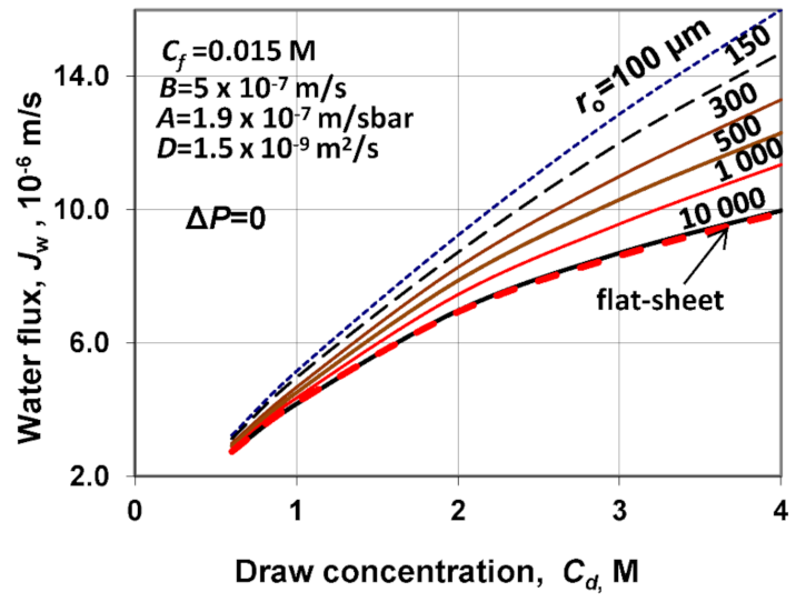
The basic idea of this energy production process is to apply a seawater–river water pair at close vicinity to the sea coast. The latest investigations showed that commercially available membrane properties and operating costs could not be profitable under the present conditions [12,13] This is why a brief discussion of the effect of draw side concentration might be useful. The effect of the draw side solute concentration on the water flux is plotted in Figure 2 at different values of the membrane lumen radius between 100 and 10,000 μm. The effect of the variable cylindrical space on the water flux at different values of the radius is the main point of this study, since the concentration’s effect is a flat-sheet mass transfer that is also already known from the literature [24]. The enormous effect of the r_o values on the water flux is seen. Its values are strongly increasing with the stronger curvature of the membrane, i.e., with the decrease in the membrane radius. For instance, the values of the water flux are 9.9 × 10⁻⁶ m/s, at r_o = 10⁴ μm (or at flat-sheet membrane) and 16 × 10⁻⁶ m/s, at r_o = 100 μm, and C_d = 4 M. This means 1.6-fold of increase on the “density” of performance. This change is rather remarkable and non-negligible, e.g., in the performance prediction of the scale-up of the industrial apparatus. On the other hand, the deviation in the water flux in the function of the membrane radius gradually decreases with the lowering of the radius. At C_d = 0.6 M, this difference falls between 2.74 × 10⁻⁶ m/s and 3.23 × 10⁻⁶ m/s, which is not more than 18%. However, it should be noted that the change in the water flux as a function of the lumen radius also depends on membrane transport parameters, such as water and salt permeability, or structural parameter and the value of the thickness of the membrane support layer, δ_d. These effects will be shown later. The water flux results obtained by the flat-sheet membrane, applying Equation (36), give excellent agreement with those obtained by the presented approached model at r_o values of 10,000 μm. This is 1 cm, which corresponds to the radius of the tube membranes. Accordingly, the cylindrical effect might already be neglected at this scale.

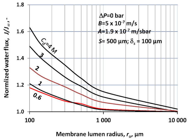
The same predicted results, like those used in Figure 2, are plotted in Figure 3 as a function of the membrane radius. This figure shows more clearly the effect of the membrane radius. As can be seen, the relative value of the water flux increases, with a decreasing lumen radius in the size range up to 1000 μm. The lumen radius of the capillary membrane modules, available at industrial-scale, generally falls between 100 μm and 200 μm. This size range has practically the highest effect of the mass transport rates due to the cylindrical space. Accordingly, leaving this effect out of consideration can cause false evaluation of the membrane performance. Later in this study, this effect will be discussed by applying measured data taken from the literature.

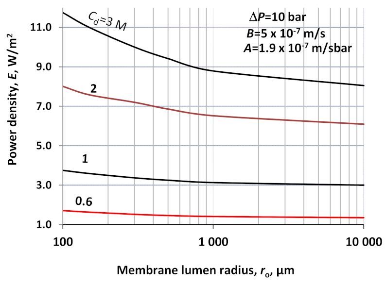
As expected, the power density varies as a function of the lumen radius with a similar tendency as it was obtained for the water flux without hydraulic pressure difference (Figure 4). With an increasing concentration of the draw solute, its effect increases on the power density as a function of the radius. The power density increase reaches about 47%, at C_d = 3 M in the radius range investigated, its values are 11.8 W/m² and 8.05 W/m², in the radius range of 100 and 10,000 μm. In studying the effect of the parameters of membrane properties, it can be seen that the effect of the radius on the produced energy density can strongly depend on them, as will be shown later in this paper.

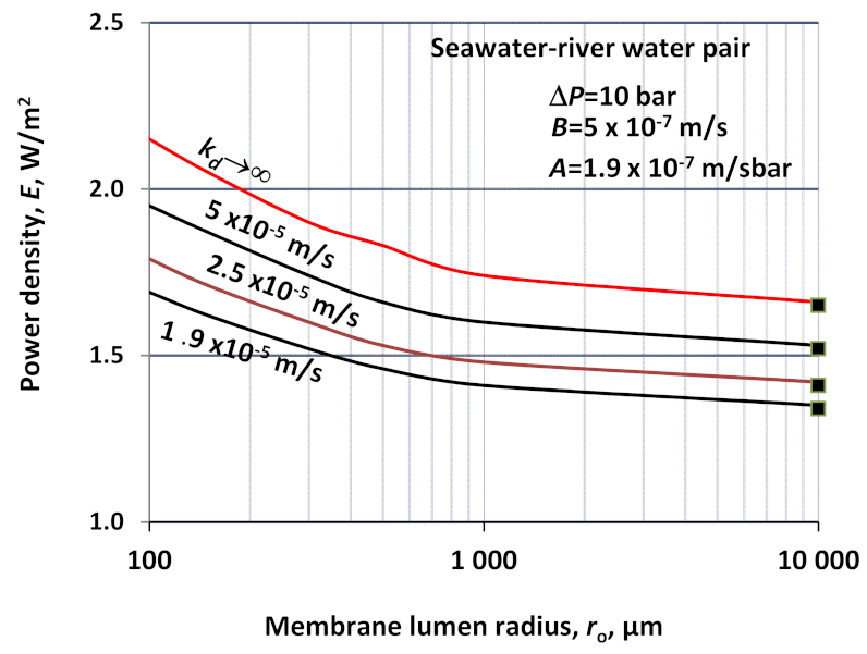
4.1.2. Effect of the Solute Transfer Coefficient, k_d, on the Power Density

Only a single figure (Figure 5) illustrates the effect of the mass transfer coefficient as a function of the lumen radius, applying for different k_d values (note k_f → ∞). As can be seen, the draw side mass transfer coefficient values also have remarkable effect on the power density, which depends rather strongly on the lumen radius. The mass transfer coefficient is mainly determined by the hydrodynamic conditions of the fluid phase. In case of a moderately stirred draw phase or at the moderate fluid flow rate of about 25–35 cm/s, the mass transfer coefficient is measured to be 1.5–1.9 × 10⁻⁵ m/s [5]. As can be seen, the value of power density is essentially lower at k_d = 1.9 × 10⁻⁵ m/s than, e.g., without mass transfer resistance in the draw fluid phase. On the other hand, the curvature of the curves in Figure 5 is similar to a function of the radius, at different values of k_d. Deviations of the curves at, e.g., k_d = 2.5 × 10⁻⁵ m/s and 5 × 10⁻⁵ m/s, are about 9% and 8%, at membrane radius of 100 μm and 10,000 μm, respectively. This means that the effect of the k_d values hardly depends on the membrane lumen radius.

4.2. Effect of the Membrane Properties, A, B and S

The main determined membrane properties are water permeability, A, solute permeability, B, and the structural parameter, S. The values of A and B as the membrane intrinsic parameters are determined experimentally by reverse osmosis measurements using the conventional methods to it [9,29]. There is not any experimental method known yet for the determination of the structural parameter, due to the soft material of the polymer membrane. This is why its prediction is carried out by means of, e.g., PRO experimental data evaluation, by applying the mathematical model developed for the flat-sheet membrane and taking into account the effect of all important mass transfer layers, as external boundary layers, and the active membrane layers as well as the porous support layer during the evaluation [4,5]. Equation (36) can also be used, though it neglects the effect of the feed side boundary layer. The structural parameter is a characteristic property of the membrane support layer. It involves the thickness, δ_s, the tortuosity, τ, and the porosity, ε, of the membrane support layer, namely S = δ_sτ/ε. Models involve the S values and, accordingly, the thickness of the support layer should be measured separately. Knowledge of its value is important during our evaluation methodologies, considering the effect of the lumen radius.

4.2.1. The Effect of the Membrane Water Permeability

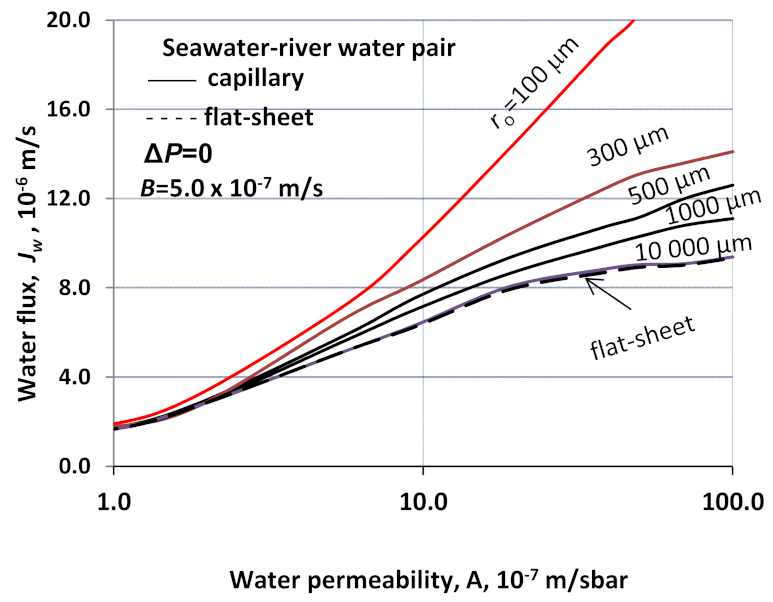
The water permeability is perhaps the most important property of a PRO (or forward osmosis, FO) membrane. It is desired to have as high value as possible. A = 1.9 × 10⁻⁷ m/sbar, listed in Table 1 is a rather low value. The measured data are similar or 2–3 fold higher. Figure 6 illustrates the effect of the A value in rather a wide range, and it is varied between 1 × 10⁻⁷ and 100 × 10⁻⁷ m/sbar.

The effect of water permeability is shown in Figure 6, which displays the change in the water flux as a function of A, at different r_o values. The increasing tendency of the water fluxes is similar to each other, at the different values of r_o. The lifting gradient of the increase in curves starts to slow at higher permeability values, due to the rapid solution of the draw solution at higher values of A.

Note that at low water permeability values, the cylindrical effect disappears almost entirely. On the other hand, the deviation between water flux curves gradually grows. For example, at A = 50 × 10⁻⁷ and 1 × 10⁻⁷ m/sbar, the increase in J_w values is 344% (J_w = 20.4 × 10⁻⁶ m/s and 8.92 × 10⁻⁶ m/s) and 14%, respectively, related to the J_w data for r_o = 100 μm and those for flat-sheet membrane, respectively. This behavior proves that the cylindrical membrane’s water flux can be remarkably affected by the cylindrical space, depending on the lumen radius. 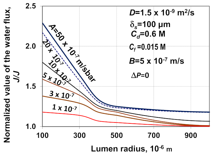This change is illustrated more clearly by Figure 7, which gives the normalized water flux (J/J_∞) vs. lumen radius at different water permeability values. As can be seen, the main change occurs below r_o < 500 μm. This is in harmony with data obtained at different values of draw side solute concentration (Figure 2). The simple cause of it is that the space variation gradually increases with the decrease in the radius. It reaches its highest value at the lowest radius, here at r_o = 100 μm. Capillary membrane modules with lesser radius (lesser than 100 μm) cannot probably be produced.

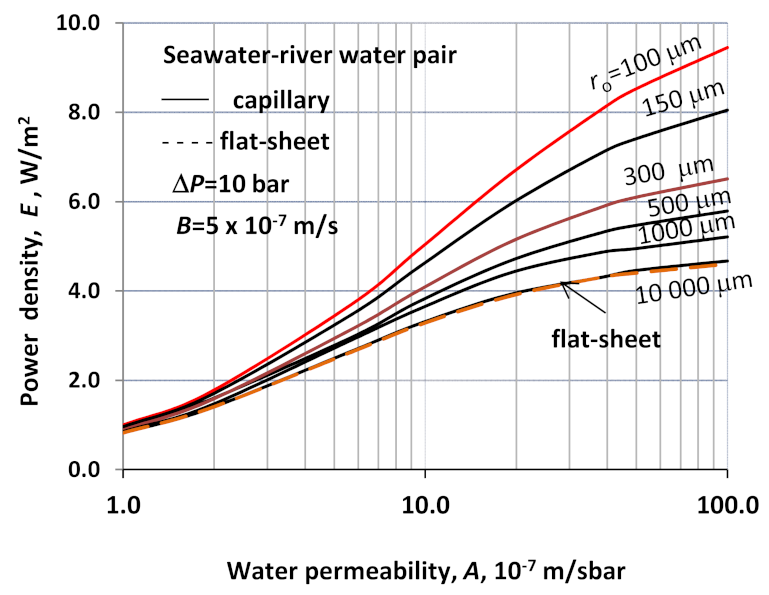
The energy density is also an important parameter, considering the membrane radius since it determines how the membrane performance is affected by the membrane radius. Figure 8 illustrates the power density as a function of the water permeability, at different values of the lumen radius, varied between r_o = 100 μm and the flat-sheet membrane at ΔP = 10 bar. Here it can also clearly be seen that the increasing tendency of the power density is rather prominent, especially in a water permeability range of (3–30) × 10⁻⁷ m/sbar. The water flux and, accordingly, the power density gradually increases with the decrease in the lumen radius. Thus, it is obvious that the lowest possible radius can serve the maximum value of the membrane performance, related to the membrane surface. Perhaps it is worth mentioning that the increase in the power density reaches close to 200% at a hydraulic pressure difference of ΔP = 10 bar, and at A = 50 × 10⁻⁷ m/sbar, considering radius values of r_o = 100 μm and 10,000 μm or for the flat-sheet membrane (values of power density obtained were 8.53 W/m² and 4.4 W/m², respectively). Note that the total surface of a capillary module with a lower radius is obviously lower than a capillary with a larger radius. Here, the performance values are compared to the surface of a capillary module. It is thought that the water flux values and the power density are characteristic parameters for the judgment of the membrane performance.

4.2.2. Effect of the Salt Permeability, B

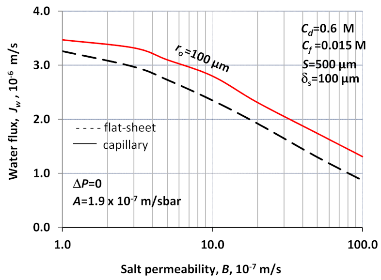
The solute permeability, as an intrinsic parameter, is also an important property of the membranes for energy generation. Producers cannot prepare a membrane with perfectly rejected property (B = 0). Even the B value is noted to change proportionally with the value of the water permeability in the case of polymeric membranes [30,31,32]. How the change in B value varies the membrane performance, using the capillary membrane is illustrated in Figure 9. The solute permeability was assumed to change between 1 × 10⁻⁷ and 100 × 10⁻⁷ m/s. Taking into account the expression of Yip and Elimelech [30], namely that B = ξA³ (ξ is a constant), the value of B can vary in a wide range depending on A values in a polymeric membrane. According to this figure, the water flux decreases relatively remarkably when B > 4 × 10⁻⁷ m/s, but one should keep in mind the values of other parameters as they are given in Table 1.

Decrease in the water flux is rather considerable in the B value range investigated; this variation is more than 300%. Comparing it to that in the function of A, it is somewhat less (see Figure 6). On the other hand, its radius dependency is relatively moderate; it is not more than about 30%, and it increases with the increase in the B value. Its absolute value lowers with the increase in B value. At least, it can be stated that one should endeavor to produce a membrane with perfect rejection property, or with solute selectivity close to 100%.

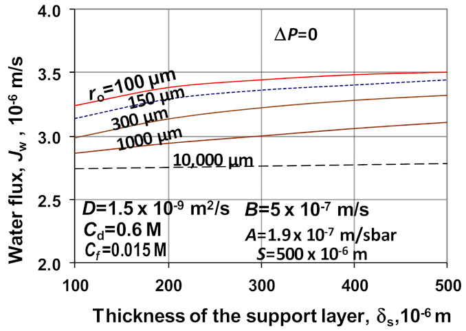
4.2.3. Effect of the Thickness of the Porous Support Layer, δ_s

During the evaluation of the measured data in the PRO system, it is a common practice to consider that the mass transport takes place through the porous membrane, and the structural parameter characterizes the support layer. This parameter is a product of the thickness, the tortuosity and the porosity, accordingly S = δ_sτ/ε. It is generally accepted that the value of τ/ε can vary between 2 and 7. In this study, it would be important to know the real thickness of the porous support layer. Due to the special investigation of this process in the literature, this value is not given in the published papers. According to our measurements, it varies between about 100–300 μm. In this study, the S value was chosen to be 500 μm, while the thickness of the membrane porous layer is 100 μm, in most of our simulation data. Here, in this subsection, δ_s was changed between 100 μm and 500 μm, while the value of S was kept at 500 μm. Accordingly, the value of τ/ε varied between 1 and 5.

Figure 10 illustrates the change in the water flux as a function of the thickness of the membrane’s structural layer, at different values of the membrane radius between 100 μm and 10,000 μm (this last value, as it was shown in some cases, corresponds to values of the flat-sheet membrane. The effect of the δ_s on the water flux is perhaps moderate (at r_o = 100 μm, the increase in water flux is not more than 9%). As it has been experienced, at r_o = 10,000 μm (or obtained by a flat-sheet membrane), the effect of the support layer curvature does not practically affect the value of the water flow rate (broken line). This means that, decisively, the lumen radius, and, accordingly, the inlet mass transfer rate, affects the overall solute transfer rate and the water flux.

Summarizing the results shown in this study, the capillary radius (i.e., the lumen radius of the asymmetric membrane) can strongly affect the water flux, and thus the membrane performance. Its effect must not be left out of consideration. If one wants to predict more precisely, e.g., during planning of the scale of an industrial task, the effect of the curvature of the membrane layer is worth taking into account. Namely, the effect of the lumen radius can reach 100% or more, depending on the mass transport parameters, such as water permeability and draw solute concentration. On the other hand, the most commercially available modules are capillary ones, with rather small lumen radius values, mostly below 200–300 μm, which is the most sensitive size range, regarding the water flux and the membrane performance.

4.3. Comparison of the Measured and Predicted Data

The measured and the predicted data were compared by applying data published by Wang et al. [18] and Wan and Chung [33]. Both research groups have measured the transport by PRO process using a hollow fiber membrane as well as applying the mathematical model by Equation (37) developed for the plane-sheet membrane.

4.3.1. Validation of the Cylindrical Model by Measured Data

As it was shown previously, the cylindrical effect can essentially alter the mass transport process depending on the values of the transport parameters as, e.g., water–, and solute permeability, operation conditions such as the inlet solute concentrations of fluid phases, and the mass transfer coefficient of the fluid phases. In the practice of evaluating the experimental data, the measured water flux is usually applied to determine the value of the structural parameter, which is difficult to be determined experimentally. The performance of a membrane layer can then be characterized. Chou et al. [18] as well as Wang et al. [19] have discussed in two papers the mass transport through hollow fiber membranes, and the water flux data were used to determine the value of the structural parameter. The measured data obtained, however, have been evaluated by means of mathematical transport models developed by flat-sheet surface. Accordingly, the structural parameter obtained does not involve the cylindrical effect. Thus, these results offered excellent possibility to be evaluated by the cylindrical model presented. Perhaps it is worth the model, used by authors of the cited paper, to be given here for the pressure retarded osmosis process (PRO):

$$J_w=K\ln \left(\frac{A{\pi }_d-J_w+B}{A{\pi }_f+B}\right)$$

(37)

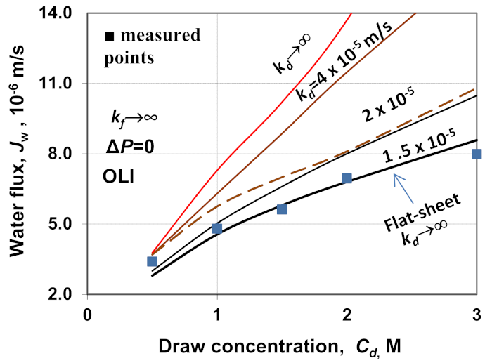
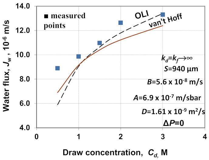
As discussed, Equation (37) does not contain the effect of the mass transfer resistances of the fluid boundary layers. The effect of the feed side boundary layer is practically negligible (its effect is generally not higher than 5–8% due to the lower concentration value; that is why our developed model has also neglected the resistance effect of mass transfer of the feed side fluid), but the effect of the draw side resistance is often remarkable. Its negligence can often cause false or faulty results in the structural parameter values, as will be illustrated later. The measured points (■) (Wang et al., Figure 7b in [18]) and the calculated water flux (broken line: the OLI software predicted the osmotic pressure; continuous line: the osmotic pressure was predicted by the van’t Hoff equation), applying Equation (37) are plotted in Figure 11, obtained for the flat-sheet membrane.

The two prediction methods show a certain deviation from each other. It follows from the fact that the van’t Hoff prediction overestimates the osmotic pressure up to about 1.0 M draw concentration. At the same time, it underestimates the osmotic pressure at higher values of solute concentrations (continuous line). Our predictions are made by the more accurate OLI software, in the following, because this software predicts the real values of the osmotic pressure. On the other hand, the predicted data are somewhat higher than the measured data, as reported by the authors in Ref. [18]. Altogether, it can be seen that the predicted values are slightly lower than the measured ones, though the external mass transfer resistances were neglected. Perhaps the OLI software application for predicting the application of osmotic pressure gives acceptable agreement with the measured ones. The remarkable discrepancy is shown at the first draw concentration, i.e., at C_d = 0.5 M.

In Figure 12, the OLI software is applied for the evaluation of the measured results published by Wang et al. [18] in Figure 7a. The effect of the draw concentration on the water flux is obtained by the cylindrical model (by Equation (31)) at r_o = 940 μm and δ_s = 150 μm, while Equation (37) was applied for the flat-sheet operation mode. The measured values (■) and their evaluation by the flat-sheet model (Equation (37)) in case of k_d = k_f→∞ are plotted by a broken line. The predicted data fit well with the measured one. On the other hand, the application of the developed cylindrical model gives much higher values than the measured ones at k_d = k_f → ∞ (dotted line), which is more significant than that in Figure 3, in the lumen radius, of r_o = 940 μm. Might it be the consequence of the neglect of the mass transfer resistance of the draw side? The question arises whether the draw side boundary layer^’s external mass transfer resistance causes this large deviation. For illustration, the effect of k_d, the water flux as a function of draw concentration, is plotted in this figure, under different values of external mass transfer coefficients. The effect of the draw concentration on the water flux is obtained by the cylindrical model (by Equation (31)) at r_o = 940 μm and δ_s = 150 μm. Water flux, predicted by the model given by Equation (31) with three different values of k_d (k_d = 1.0, 1.5, 4.0 and →∞; k_f was assumed to be infinite in every case), can be strongly affected by the values of k_d, its decrease gradually lowers the deviation of the predicted data from those of the measured ones.

The question can be whether the k_d value can be neglected at Re = 1500 (Re = v2r_o/D) as it was done by the authors in Ref. [18]. Accordingly, the volume flow rate is 0. 5 cm/s (5 × 10⁻³ m/s), which is a rather low value. Bui et al. [5] measured the values of the external mass transfer coefficients, k_d, and k_f and they have obtained that k_d = 1.74–1.84 × 10⁻⁵ m/s and 2.0–2.1 × 10⁻⁵ m/s for 0–1.5 M NaCl with cross-flow velocities between 0.21–0.31 m/s. Manickam and McCutcheon [10] reported similar results, namely k_d = 2.0 × 10⁻⁵ m/s at 0.26 m/s cross-flow velocity. In this case, however, the volume velocity in the capillary is much lower. However, the convective velocity of 0.5 cm/s cannot provide remarkable dispersion; thus, the streaming can remain laminar in that the transfer resistance can strongly alter the transfer rate of the solute and water (if Re < 2100–2300 then the flow in the capillary is laminar). Applying the Graetz–Léveque expression for the determination of the Sherwood number, i.e., Sh = (ReScd/L)^0.33 [24], the mass transfer coefficient of the draw side will be as k_d ≅ 1.2 × 10⁻⁵ m/s. The water flux for this mass transfer coefficient is also plotted in Figure 12 (dot-dot-broken line). In our opinion, these predicted results are close to the measured one, proving the applicability of the cylindrical model presented. According to these results, it is needed to compare the results of the presented model with other measured data.

4.3.2. Model Validation by Measured Data of Wan and Chung

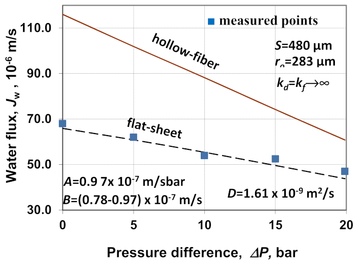
Figure 13 represents the measured data reported by Wan and Chung [33], who measured the effect of the hydraulic pressure difference on the water flux [Figure 6a in Ref. [33], (■)], applying the hollow fiber membrane during the PRO process. The OLI software is applied for the evaluation of the measured results published by these authors. The measured square points and their evaluation by the flat-sheet model (Equation (37)) in case of k_d = k_f → ∞ is plotted by a dashed line (C_d = 1 M NaCl; C_f = 0). The values of A (A = 9.7 × 10⁻⁷ m/cbar = 3.5 Lmh) and B (B = 0.78 m/s − 0.97 × 10⁻⁷ m/s = 0.28 Lmh − 0.35 Lmh as a function of the pressure difference) were measured by the authors. The value of the structural parameter was obtained by fitting the model data to the measured ones. Thus, it was obtained that S = 480 µm. As it can be seen, the measured and the predicted data have an excellent agreement. The effect of the hydraulic pressure difference on the water flux, predicted by using the cylindrical model (by Equation (31)) at r_o = 288 μm and δ_s = 225 μm is plotted by a solid line.

As it clearly can be seen in Figure 13, the predicted water flux data are significantly higher, taking into account the cylindrical effect, than the measured one. The cylindrical effect decreases in some measure. The deviation between the measured and the predicted data decreases as a function of ∆P with the increase in the hydraulic pressure difference. The difference between the measured values and that of the cylindrical model reaches 72%, which decreases to 39%, with the increase in the ∆P (from zero to 20 bar).

Summarizing the message of this paper, the developed mathematical model for the cylindrical membrane clearly shows the strong effect of the radius of the hollow fiber membrane on the mass transport through a capillary membrane layer. Technologists and engineers can easily use the relatively simple application of the presented mathematical model given in closed form for membrane performance as a function of the lumen radius and membrane thickness. This cylindrical model should give more correct performance results for hollow fiber modules than that developed for the flat-sheet membrane.

5. Conclusions

The overall solute and the water flux can essentially be affected by the cylindrical effect of a hollow fiber membrane, where the transfer surface and the differential membrane volume are a strong function of the membrane radius. An approach by the cylindrical mass transport model has been developed and solved, which was then applied to show the variation in water flux as a function of the membrane radius, using different membrane transport properties (A, B, δ_s membrane thickness) and operating conditions (C_d, k_d). It was stated that the inlet solute concentration strongly influences the water flux, depending on the lumen radius. In the lumen radius range of 150–1000 μm, this change can reach 200–300%, depending on the draw concentration. Similarly, the water permeability also strongly affects the water flux, depending on the lumen radius. The change in the power density can reach 4–6 fold or more with the increase in the water permeability and/or with a decrease in the lumen radius. According to Figure 13, the power density obtained by using a cylindrical membrane is 66% more than that by using a model for a flat-sheet membrane applying the same values of the transport parameters. The major statements in this paper, according to the results are as follows:

• the mass transfer rate (solute and water) through the cylindrical membrane essentially differs from that of the flat-sheet membrane;
• the deviation strongly depends on the membrane radius between r_o = 150–1000 µm, depending on the values of the transport parameters (A, B, S, k_d);
• with the decrease in the membrane radius, the cylindrical effect increases and the increase can reach 4–6 fold;
• the developed cylindrical mathematical model serves as a simple iterative calculation method for the prediction of the cylindrical membrane performance.

Applying the transport equation developed for a flat-sheet membrane must not be recommended to evaluate water flux data obtained by the capillary membrane layer. The correct prediction of membrane performance by capillary membrane demands the application of the cylindrical model. An important advantage of the cylindrical model is that the membrane performance can be predicted more precisely. Thus, it makes possible the more accurate planning of a large-scale apparatus.