
Blockage Corrections for Tidal Turbines—Application to an Array of Turbines in the Alderney Race


Abstract
:1. Introduction
2. Materials and Method
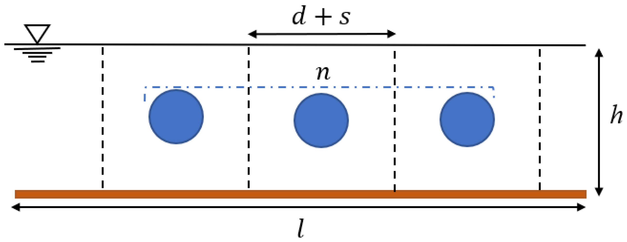
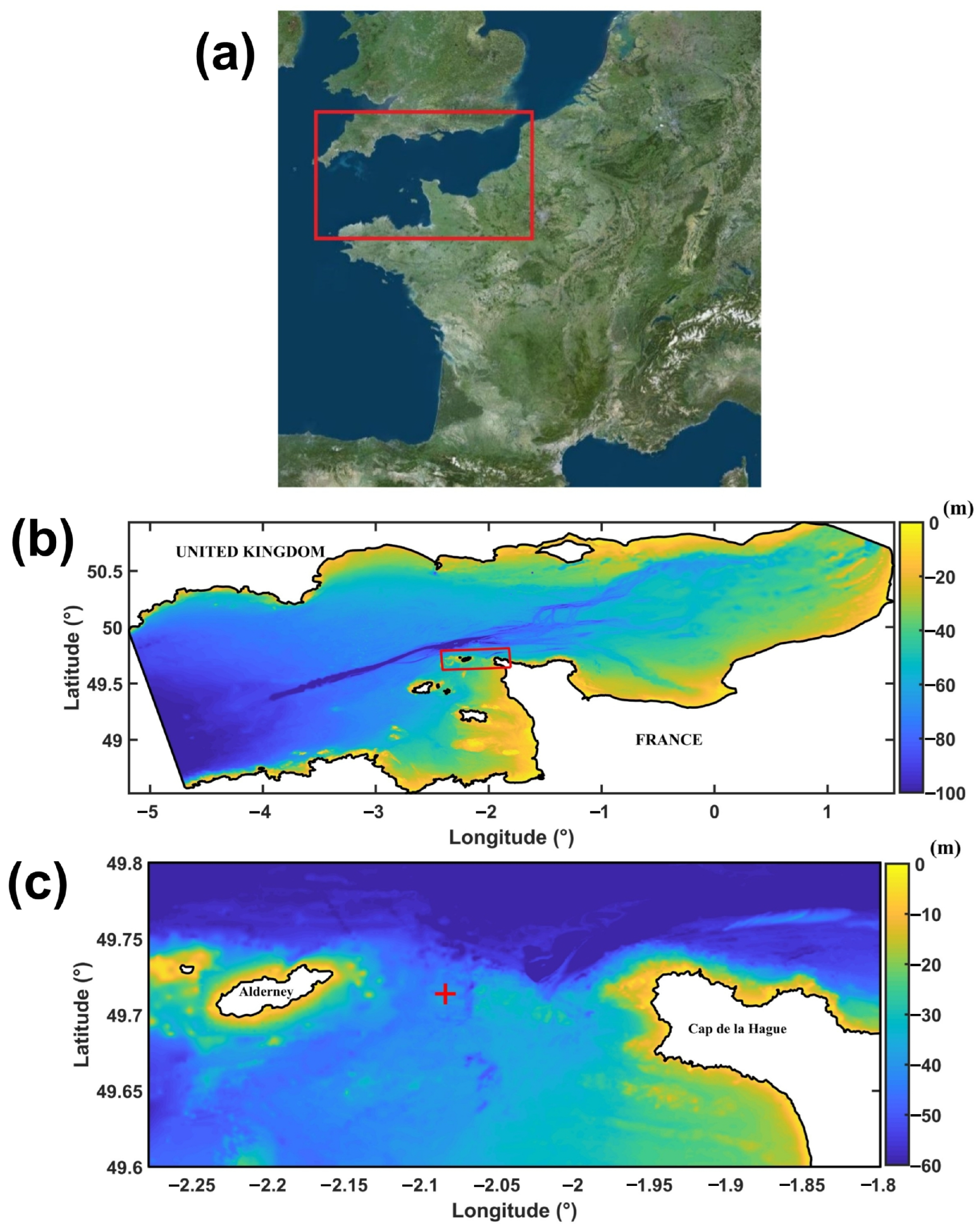
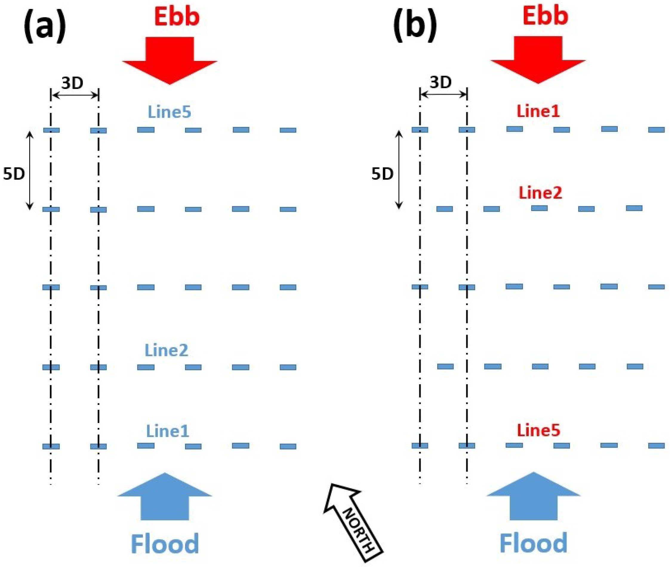
2.1. Study Site and Turbine Array
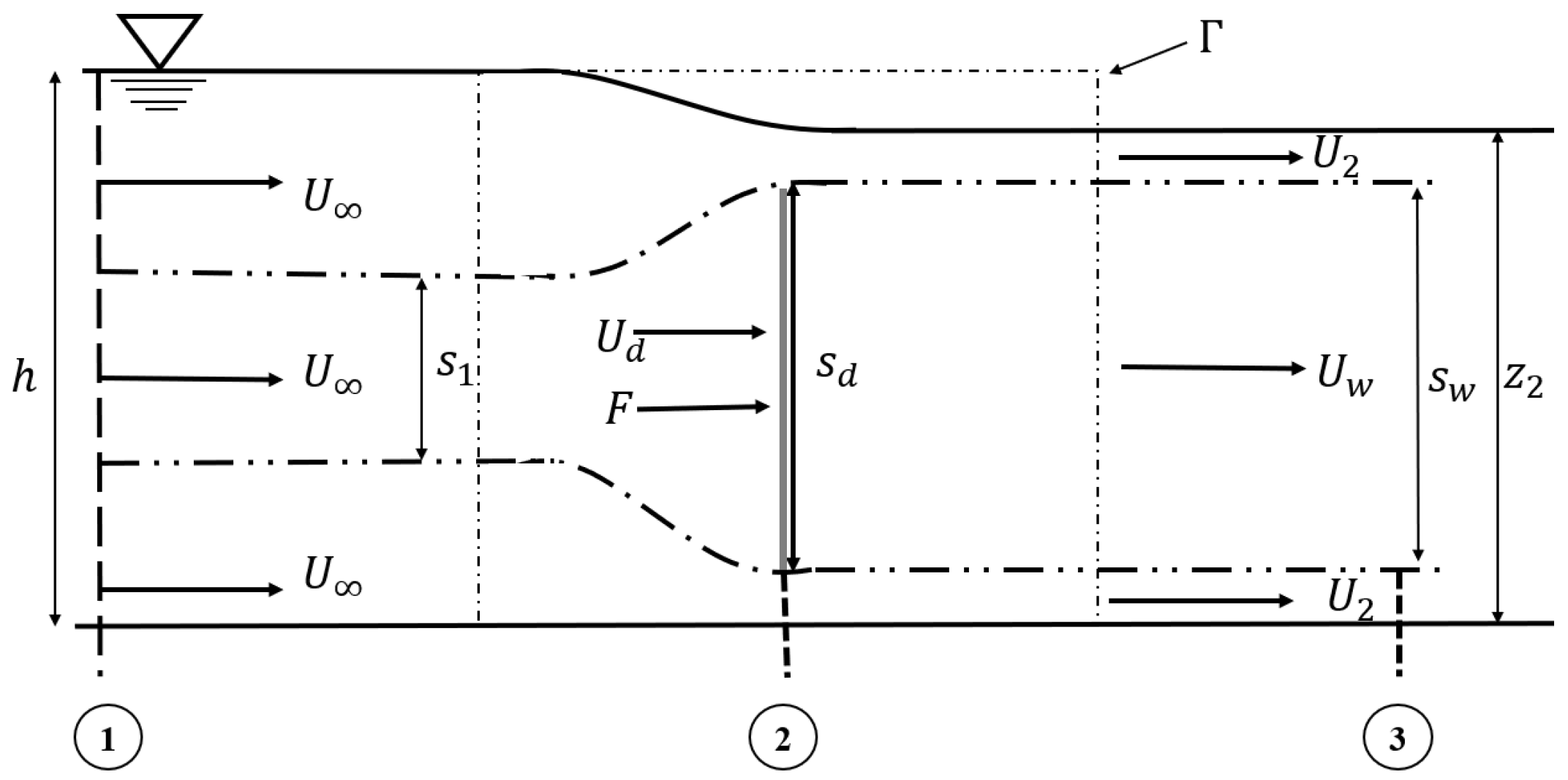
2.2. Analytical Model
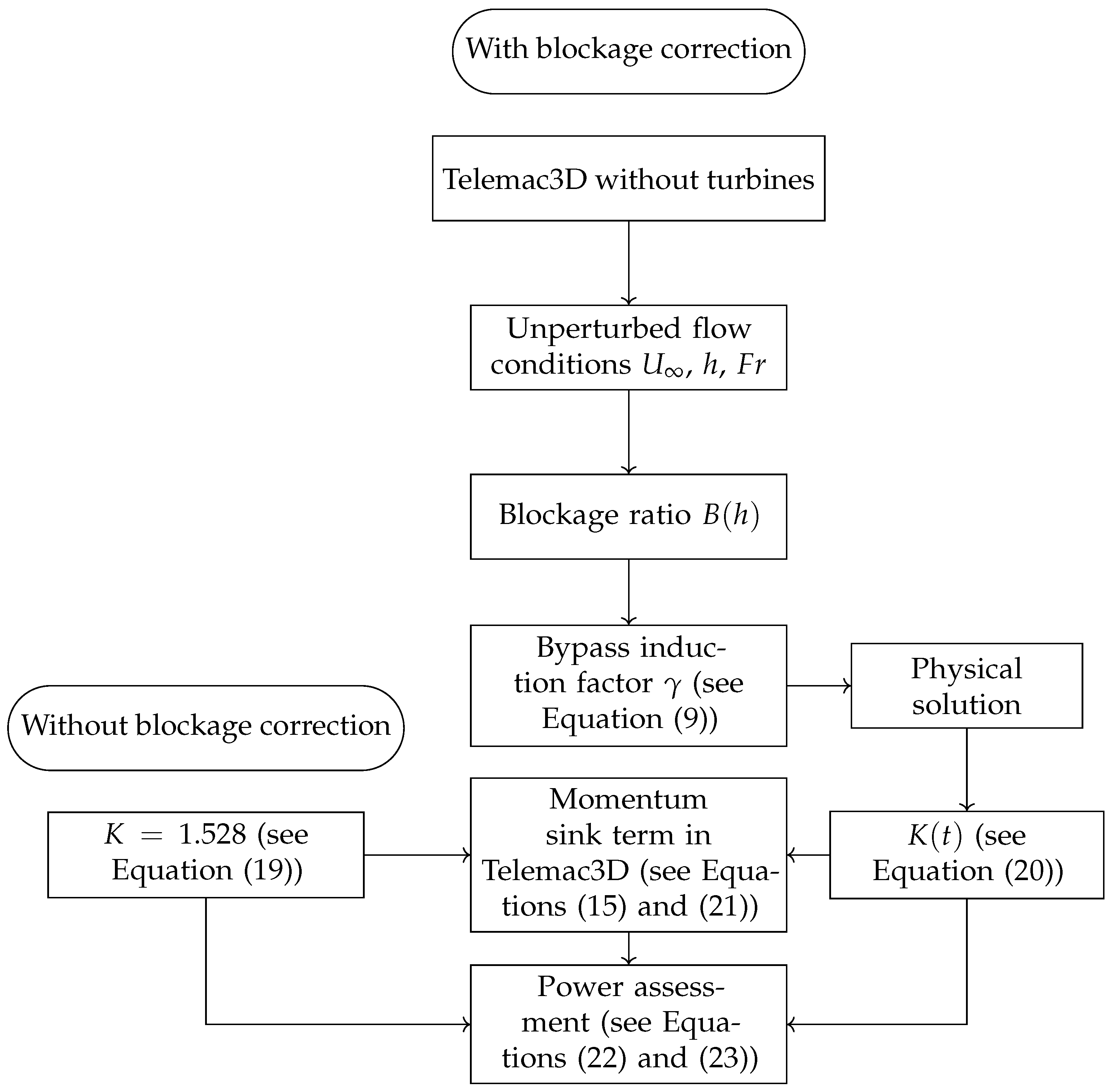
2.3. Numerical Model
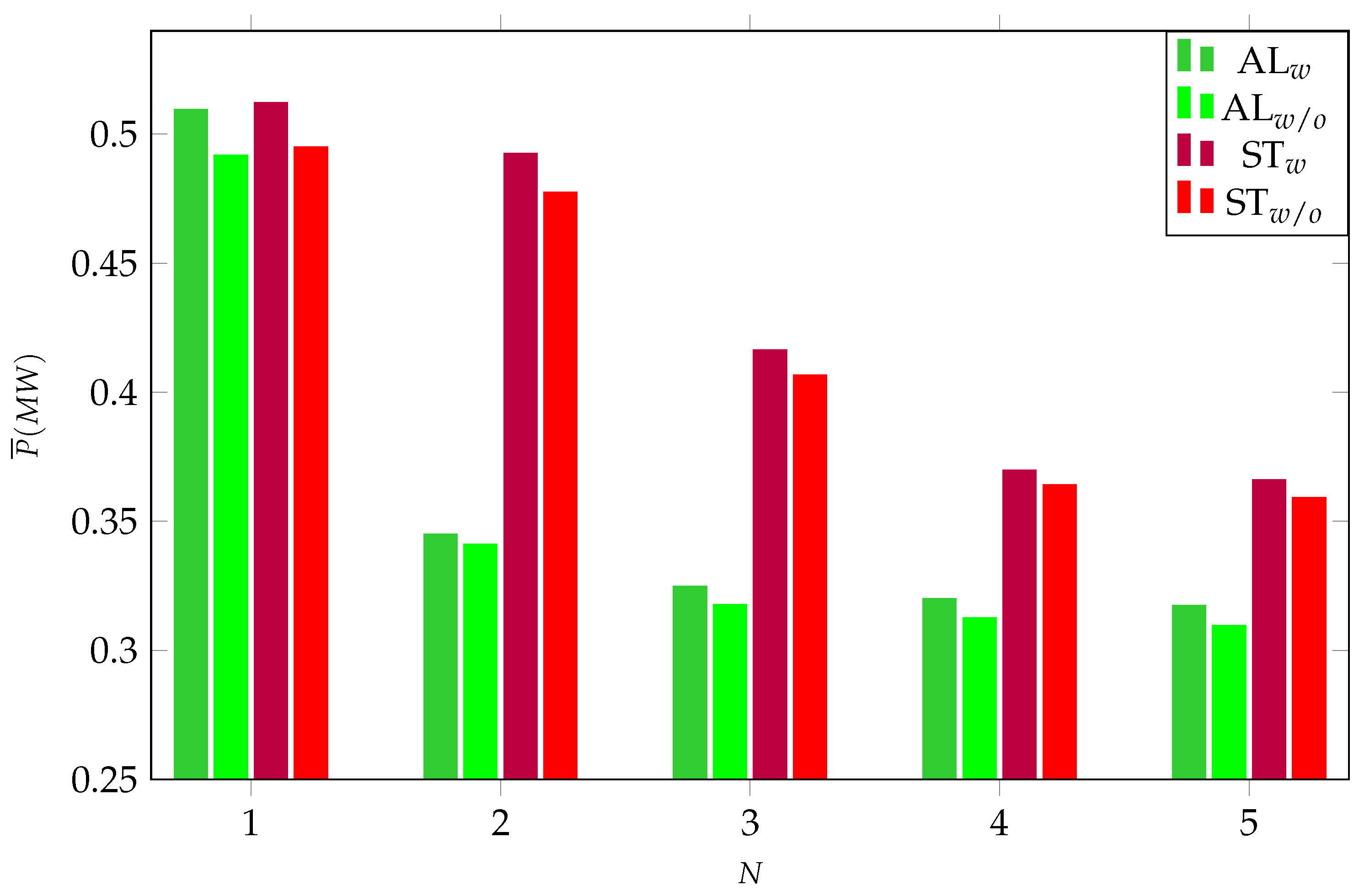
3. Results and Discussion
4. Conclusions
Author Contributions
Funding
Institutional Review Board Statement
Informed Consent Statement
Data Availability Statement
Acknowledgments
Conflicts of Interest
Abbreviations
| Ratio of the downstream to the upstream velocity, dimensionless | |
| Ratio of the velocity in the disc to the upstream velocity, dimensionless | |
| Bypass induction factor, dimensionless | |
| Blockage ratio, dimensionless | |
| Water density, kg/m | |
| Effective kinematic viscosity, m s | |
| Pressure drop across the disc, kg m s | |
| Free surface elevation, m | |
| A | Area swept by the blades, m |
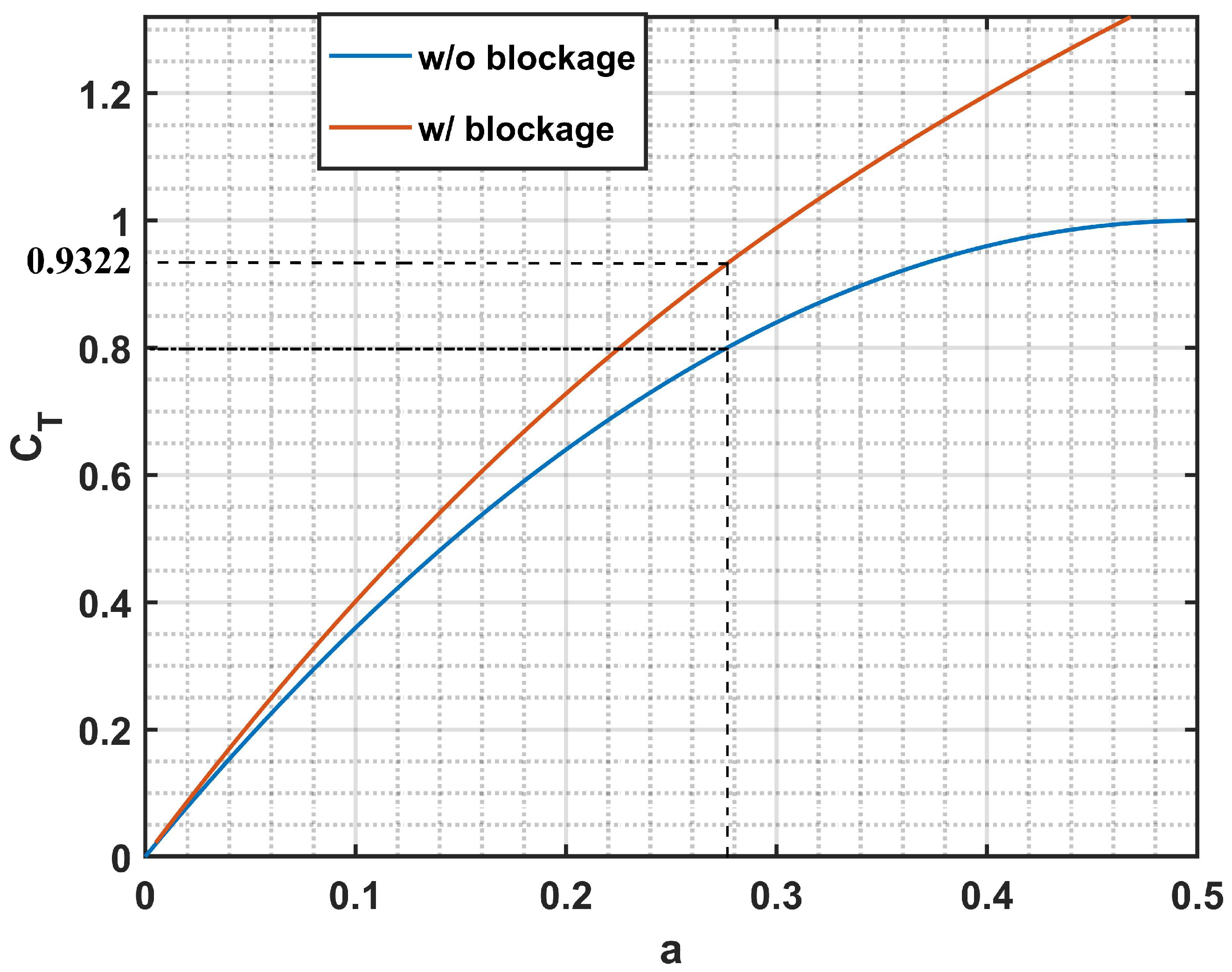
| a | Axial induction factor, dimensionless |
| Thrust coefficient, dimensionless | |
| Power coefficient, dimensionless | |
| e | Thickness of the disc, m |
| F | Thrust force, kg m s |
| Froude number, dimensionless | |
| g | Acceleration of the earth’s gravity, m/s |
| h | Water depth, m |
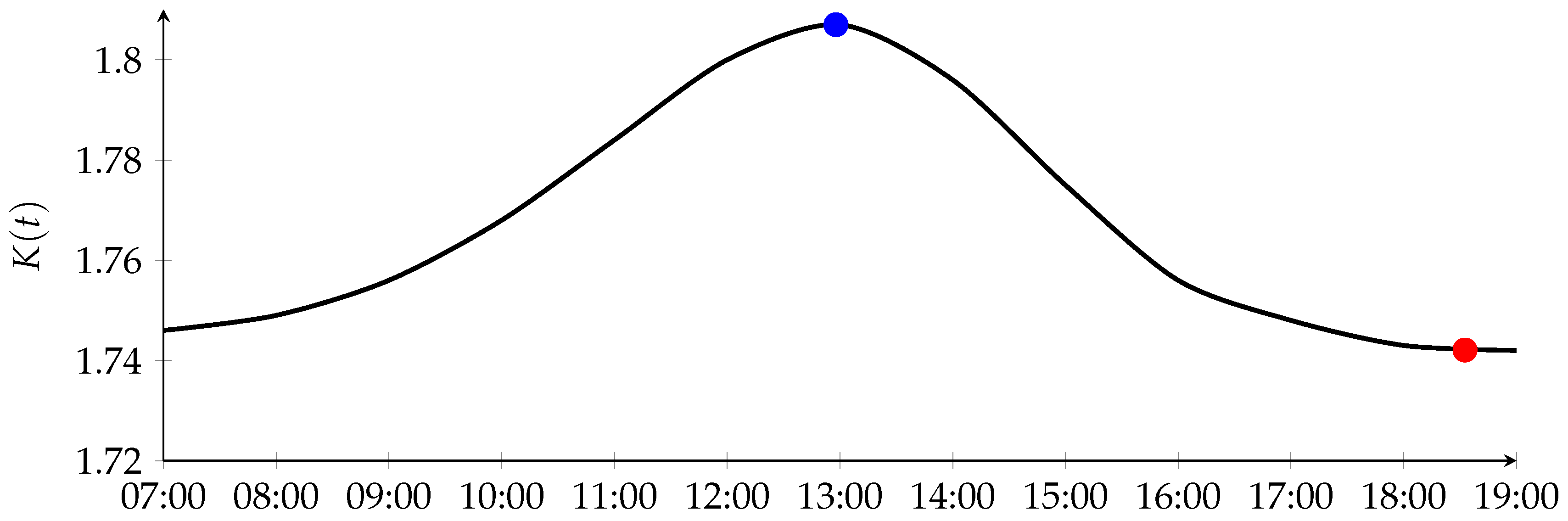
| K | Resistance coefficient, dimensionless |
| l | Transverse width of the flow, m |
| Atmospheric pressure, kg m s | |
| Upstream area of the actuator disk per unit transverse width of the flow, m | |
| Area of the actuator disk per unit transverse width of the flow, m | |
| Far downstream area of the actuator disk per unit transverse width of the flow, m | |
| , S, S | Source terms, kg m s |
| t | Time, s |
| Upstream velocity, m s | |
| Velocity in the disc, m s | |
| Velocity in the far downstream, m s | |
| Velocity in the far wake, m s | |
| u, v, w | Three components of the velocity, m s |
| Water depth, m |
References
- Myers, L.; Bahaj, A. Simulated electrical power potential harnessed by marine current turbine arrays in the Alderney Race. Renew. Energy 2005, 30, 1713–1731. [Google Scholar] [CrossRef]
- Myers, L.E.; Bahaj, A.S. An experimental investigation simulating flow effects in first generation marine current energy converter arrays. Renew. Energy 2012, 37, 28–36. [Google Scholar] [CrossRef] [Green Version]
- Roc, T.; Conley, D.C.; Greaves, D. Methodology for tidal turbine representation in ocean circulation model. Renew. Energy 2013, 51, 448–464. [Google Scholar] [CrossRef] [Green Version]
- Thiébot, J.; Guillou, S.; Nguyen, V.T. Modelling the effect of large arrays of tidal turbines with depth-averaged Actuator Disks. Ocean Eng. 2016, 126, 265–275. [Google Scholar] [CrossRef]
- Olczak, A.; Stallard, T.; Feng, T.; Stansby, P.K. Comparison of a RANS blade element model for tidal turbine arrays with laboratory scale measurements of wake velocity and rotor thrust. J. Fluids Struct. 2016, 64, 87–106. [Google Scholar] [CrossRef]
- Nash, S.; Phoenix, A. A review of the current understanding of the hydro-environmental impacts of energy removal by tidal turbines. Renew. Sustain. Energy Rev. 2017, 80, 648–662. [Google Scholar] [CrossRef]
- Plew, D.R.; Stevens, C.L. Numerical modelling of the effect of turbines on currents in a tidal channel—Tory Channel, New Zealand. Renew. Energy 2013, 57, 269–282. [Google Scholar] [CrossRef]
- Neill, S.P.; Jordan, J.R.; Couch, S.J. Impact of tidal energy converter (TEC) arrays on the dynamics of headland sand banks. Renew. Energy 2012, 37, 387–397. [Google Scholar] [CrossRef]
- Guillou, N.; Chapalain, G.; Neill, S.P. The influence of waves on the tidal kinetic energy resource at a tidal stream energy site. Appl. Energy 2016, 180, 402–415. [Google Scholar] [CrossRef] [Green Version]
- Houlsby, G.T.; Draper, S.; Oldfield, M.L.G. Application of Linear Momentum Actuator Disc Theory to Open Channel Flow; OUEL: Yao, Japan, 2008. [Google Scholar]
- Draper, S.; Houlsby, G.; Oldfield, M.; Borthwick, A. Modelling tidal energy extraction in a depth-averaged coastal domain. Renew. Power Gener. IET 2010, 4, 545–554. [Google Scholar] [CrossRef] [Green Version]
- Adcock, T.A.A.; Draper, S.; Houlsby, G.T.; Borthwick, A.G.L.; Serhadlıoğlu, S. The available power from tidal stream turbines in the Pentland Firth. Proc. R. Soc. A Math. Phys. Eng. Sci. 2013, 469, 20130072. [Google Scholar] [CrossRef] [Green Version]
- Serhadlıoğlu, S.; Adcock, T.A.A.; Houlsby, G.T.; Draper, S.; Borthwick, A.G.L. Tidal stream energy resource assessment of the Anglesey Skerries. Int. J. Mar. Energy 2013, 3–4, e98–e111. [Google Scholar] [CrossRef] [Green Version]
- Harrison, M.E.; Batten, W.M.J.; Myers, L.E.; Bahaj, A.S. Comparison between CFD simulations and experiments for predicting the far wake of horizontal axis tidal turbines. IET Renew. Power Gener. 2010, 4, 613–627. [Google Scholar] [CrossRef] [Green Version]
- Abolghasemi, M.A.; Piggott, M.D.; Spinneken, J.; Viré, A.; Cotter, C.J.; Crammond, S. Simulating tidal turbines with multi-scale mesh optimisation techniques. J. Fluids Struct. 2016, 66, 69–90. [Google Scholar] [CrossRef] [Green Version]
- Malki, R.; Masters, I.; Williams, A.J.; Nick Croft, T. Planning tidal stream turbine array layouts using a coupled blade element momentum—Computational fluid dynamics model. Renew. Energy 2014, 63, 46–54. [Google Scholar] [CrossRef] [Green Version]
- Stallard, T.; Collings, R.; Feng, T.; Whelan, J. Interactions between tidal turbine wakes: Experimental study of a group of three-bladed rotors. Philos. Trans. R. Soc. A Math. Phys. Eng. Sci. 2013, 371, 20120159. [Google Scholar] [CrossRef]
- Thiébot, J.; Guillou, N.; Guillou, S.; Good, A.; Lewis, M. Wake field study of tidal turbines under realistic flow conditions. Renew. Energy 2020, 151, 1196–1208. [Google Scholar] [CrossRef]
- Michelet, N.; Guillou, N.; Chapalain, G.; Thiébot, J.; Guillou, S.; Goward Brown, A.J.; Neill, S.P. Three-dimensional modelling of turbine wake interactions at a tidal stream energy site. Appl. Ocean Res. 2020, 95, 102009. [Google Scholar] [CrossRef]
- Nguyen, V.T.; Santa Cruz, A.; Guillou, S.S.; Shiekh Elsouk, M.N.; Thiébot, J. Effects of the Current Direction on the Energy Production of a Tidal Farm: The Case of Raz Blanchard (France). Energies 2019, 12, 2478. [Google Scholar] [CrossRef] [Green Version]
- Abolghasemi, M.A.; Piggott, M.D.; Kramer, S.C. An investigation into the accuracy of the depth-averaging used in tidal turbine array optimisation. arXiv 2018, arXiv:1810.09827. [Google Scholar]
- McTavish, S.; Feszty, D.; Nitzsche, F. An experimental and computational assessment of blockage effects on wind turbine wake development. Wind Energy 2014, 17, 1515–1529. [Google Scholar] [CrossRef]
- Bahaj, A.S.; Batten, W.M.J.; McCann, G. Experimental verifications of numerical predictions for the hydrodynamic performance of horizontal axis marine current turbines. Renew. Energy 2007, 32, 2479–2490. [Google Scholar] [CrossRef]
- Nishino, T.; Willden, R.H.J. Effects of 3-D channel blockage and turbulent wake mixing on the limit of power extraction by tidal turbines. Int. J. Heat Fluid Flow 2012, 37, 123–135. [Google Scholar] [CrossRef]
- Kinsey, T.; Dumas, G. Impact of channel blockage on the performance of axial and cross-flow hydrokinetic turbines. Renew. Energy 2017, 103, 239–254. [Google Scholar] [CrossRef]
- Kolekar, N.; Vinod, A.; Banerjee, A. On Blockage Effects for a Tidal Turbine in Free Surface Proximity. Energies 2019, 12, 3325. [Google Scholar] [CrossRef] [Green Version]
- Garrett, C.; Cummins, P. The efficiency of a turbine in a tidal channel. J. Fluid Mech. 2007, 588, 243–251. [Google Scholar] [CrossRef] [Green Version]
- Whelan, J.I.; Graham, J.M.R.; Peiró, J. A free-surface and blockage correction for tidal turbines. J. Fluid Mech. 2009, 624, 281–291. [Google Scholar] [CrossRef]
- Nishino, T.; Willden, R.H.J. The efficiency of an array of tidal turbines partially blocking a wide channel. J. Fluid Mech. 2012, 708, 596–606. [Google Scholar] [CrossRef]
- Vogel, C.R.; Houlsby, G.T.; Willden, R.H.J. Effect of free surface deformation on the extractable power of a finite width turbine array. Renew. Energy 2016, 88, 317–324. [Google Scholar] [CrossRef]
- Schluntz, J.; Willden, R.H.J. The effect of blockage on tidal turbine rotor design and performance. Renew. Energy 2015, 81, 432–441. [Google Scholar] [CrossRef]
- Flores Mateos, L.; Hartnett, M. Hydrodynamic Effects of Tidal-Stream Power Extraction for Varying Turbine Operating Conditions. Energies 2020, 13, 3240. [Google Scholar] [CrossRef]
- Thiébot, J.; Djama Dirieh, N.; Guillou, S.; Guillou, N. The Efficiency of a Fence of Tidal Turbines in the Alderney Race: Comparison between Analytical and Numerical Models. Energies 2021, 14, 892. [Google Scholar] [CrossRef]
- Campbell, R.; Martinez, A.; Letetrel, C.; Rio, A. Methodology for estimating the French tidal current energy resource. Int. J. Mar. Energy 2017, 19, 256–271. [Google Scholar] [CrossRef]
- Coles, D.S.; Blunden, L.S.; Bahaj, A.S. Assessment of the energy extraction potential at tidal sites around the Channel Islands. Energy 2017, 124, 171–186. [Google Scholar] [CrossRef]
- Bailly du Bois, P.; Dumas, F.; Morillon, M.; Furgerot, L.; Voiseux, C.; Poizot, E.; Méar, Y.; Bennis, A.C. The Alderney Race: General hydrodynamic and particular features. Philos. Trans. R. Soc. A Math. Phys. Eng. Sci. 2020, 378, 20190492. [Google Scholar] [CrossRef]
- Guillou, N.; Neill, S.P.; Thiébot, J. Spatio-temporal variability of tidal-stream energy in north-western Europe. Philos. Trans. R. Soc. A Math. Phys. Eng. Sci. 2020, 378, 20190493. [Google Scholar] [CrossRef]
- Sentchev, A.; Nguyen, T.D.; Furgerot, L.; Bailly du Bois, P. Underway velocity measurements in the Alderney Race: Towards a three-dimensional representation of tidal motions. Philos. Trans. R. Soc. A Math. Phys. Eng. Sci. 2020, 378, 20190491. [Google Scholar] [CrossRef]
- Thiébot, J.; Coles, D.S.; Bennis, A.C.; Guillou, N.; Neill, S.; Guillou, S.; Piggott, M. Numerical modelling of hydrodynamics and tidal energy extraction in the Alderney Race: A review. Philos. Trans. R. Soc. A Math. Phys. Eng. Sci. 2020, 378, 20190498. [Google Scholar] [CrossRef]
- Lo Brutto, O.A.; Nguyen, V.T.; Guillou, S.S.; Thiébot, J.; Gualous, H. Tidal farm analysis using an analytical model for the flow velocity prediction in the wake of a tidal turbine with small diameter to depth ratio. Renew. Energy 2016, 99, 347–359. [Google Scholar] [CrossRef]
- Hervouet, J.M. Hydrodynamics of Free Surface Flows: Modelling with the Finite Element Method; John Wiley & Sons: Hoboken, NJ, USA, 2007. [Google Scholar] [CrossRef]
- Kramer, S.C.; Piggott, M.D. A correction to the enhanced bottom drag parameterisation of tidal turbines. Renew. Energy 2016, 92, 385–396. [Google Scholar] [CrossRef] [Green Version]
- Taylor, G.I. The Scientific Papers of Sir Geoffrey Ingram Taylor: Mechanics of Solids; CUP Archive; Cambridge University Press: Cambridge, UK, 1958; Volume 1. [Google Scholar]
- Bahaj, A.S.; Molland, A.F.; Chaplin, J.R.; Batten, W.M.J. Power and thrust measurements of marine current turbines under various hydrodynamic flow conditions in a cavitation tunnel and a towing tank. Renew. Energy 2007, 32, 407–426. [Google Scholar] [CrossRef]
- Ouro, P.; Nishino, T. Performance and wake characteristics of tidal turbines in an infinitely large array. J. Fluid Mech. 2021, 925. [Google Scholar] [CrossRef]
- Adcock, T.A.A.; Draper, S.; Nishino, T. Tidal power generation—A review of hydrodynamic modelling. Proc. Inst. Mech. Eng. Part A J. Power Energy 2015, 229, 755–771. [Google Scholar] [CrossRef]
- Bonar, P.A.J.; Bryden, I.G.; Borthwick, A.G.L. Social and ecological impacts of marine energy development. Renew. Sustain. Energy Rev. 2015, 47, 486–495. [Google Scholar] [CrossRef]
- Ross, H.; Polagye, B. An experimental assessment of analytical blockage corrections for turbines. Renew. Energy 2020, 152, 1328–1341. [Google Scholar] [CrossRef] [Green Version]


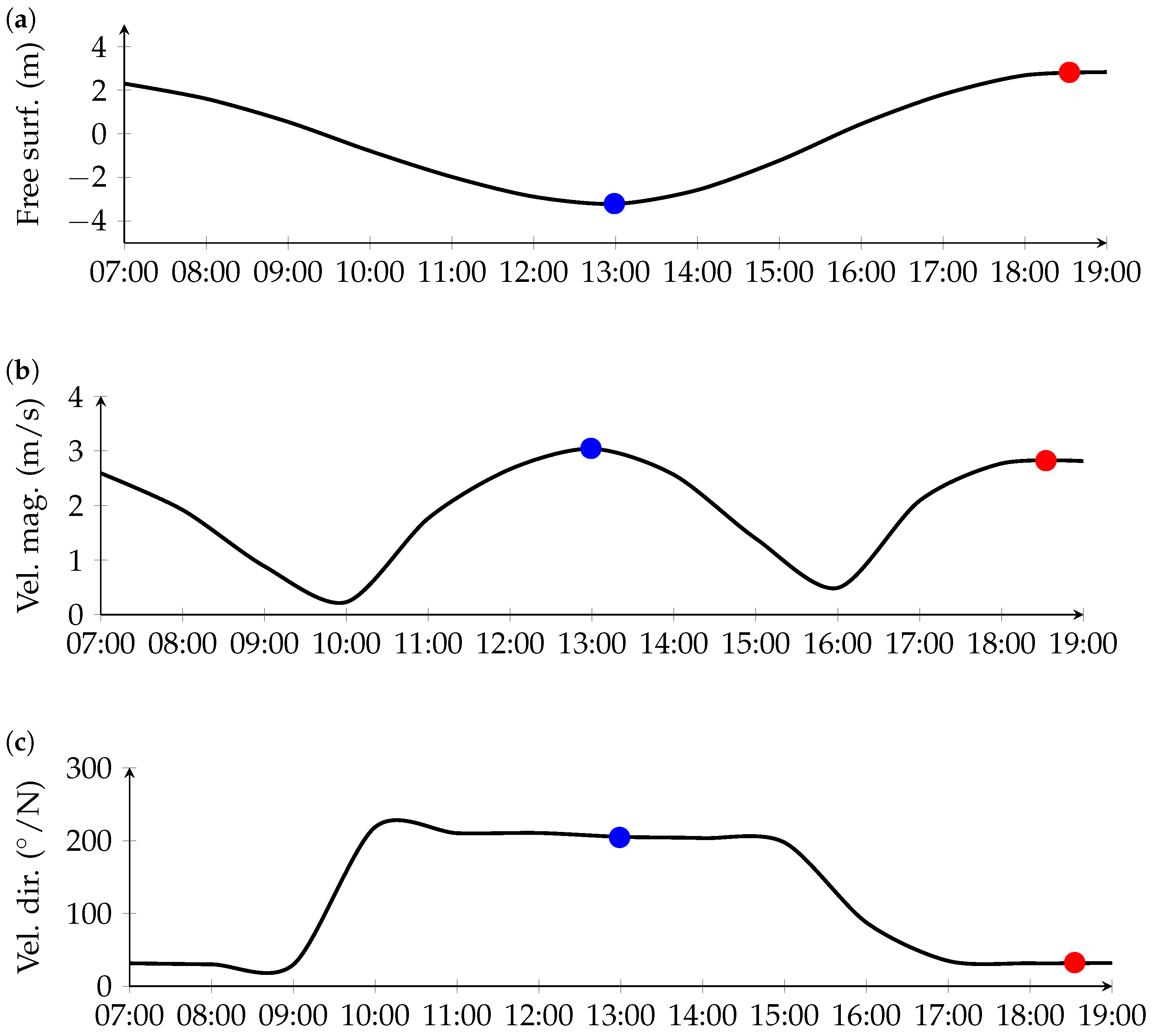
| Peak Ebb | Peak Flood | |
|---|---|---|
| Velocity magnitude (m/s) | ||
| Velocity direction (/North) | 206 | 32 |
| Water depth (m) | ||
| Froude number (dimensionless) | ||
| Local blockage ratio (%) |
Publisher’s Note: MDPI stays neutral with regard to jurisdictional claims in published maps and institutional affiliations. |
© 2022 by the authors. Licensee MDPI, Basel, Switzerland. This article is an open access article distributed under the terms and conditions of the Creative Commons Attribution (CC BY) license (https://creativecommons.org/licenses/by/4.0/).
Share and Cite
Djama Dirieh, N.; Thiébot, J.; Guillou, S.; Guillou, N. Blockage Corrections for Tidal Turbines—Application to an Array of Turbines in the Alderney Race. Energies 2022, 15, 3475. https://doi.org/10.3390/en15103475
Djama Dirieh N, Thiébot J, Guillou S, Guillou N. Blockage Corrections for Tidal Turbines—Application to an Array of Turbines in the Alderney Race. Energies. 2022; 15(10):3475. https://doi.org/10.3390/en15103475
Chicago/Turabian StyleDjama Dirieh, Nasteho, Jérôme Thiébot, Sylvain Guillou, and Nicolas Guillou. 2022. "Blockage Corrections for Tidal Turbines—Application to an Array of Turbines in the Alderney Race" Energies 15, no. 10: 3475. https://doi.org/10.3390/en15103475
APA StyleDjama Dirieh, N., Thiébot, J., Guillou, S., & Guillou, N. (2022). Blockage Corrections for Tidal Turbines—Application to an Array of Turbines in the Alderney Race. Energies, 15(10), 3475. https://doi.org/10.3390/en15103475