Method to Predict the Non-Uniform Potential Distribution in Random Electrical Machine Windings under Pulse Voltage Stress

Abstract

This article describes a practical method for predicting the distribution of electric potential inside an electrical machine’s winding based on design data. It broadens the understanding of winding impedance in terms of inter-winding behavior and allows to properly design an electrical machine’s insulation system during the development phase. The predictions are made based on an frequency-dependent equivalent circuit of the electrical machine which is validated by measurements in the time domain and the frequency domain. Element parameters for the equivalent circuit are derived from two-dimensional field simulations. The results demonstrate a non-uniform potential distribution and demonstrate that the potential difference between individual turns and between turns and the stator core exceeds the expected values. The findings also show a link between winding impedance and potential oscillations inside the winding. Additionally, the article provides an overview of the chronological progression of turn-based models and shows how asynchronous multiprocessing is used to accelerate the solution process of the equivalent circuit.

1. Introduction

As presented in a recently published article [1], research concerning non-uniform potential distributions in electrical machine windings dates back to 1930 [2] and even back to 1902 for transformers [3]. It was observed that non-uniform potential distributions occur during voltage transients at the machine terminals which impose abnormal stress on the insulation. Switching operations or lightning surges were common causes for such transients. Today, the motivation for research of high-frequency (HF) models originates from the introduction of new wide band-gap semiconductors like silicon carbide (SiC) and gallium nitride (GaN) for power MOSFETs. Those enable power inverters to operate at higher switching frequencies and higher voltage gradients $\mathrm{d}u/\mathrm{d}t$ than silicon (Si) based ones.

The successive work of scientists produced models of increasing complexity and better understanding of cause and effect of non-uniform potential distributions [4,5,6,7,8,9]. Figure 1 gives an overview of the increasing complexity and shows the foundation for the model which was derived in this article. More recent publications [10,11] pursue almost identical approaches without incorporating frequency-dependent effects. In [12,13], frequency-dependent resistance and inductance are incorporated into the model and solved in the time domain. To do so, frequency-dependent circuit elements are approximated by ladder networks. These ladder networks increase the overall count of circuit elements. Depending on the chosen order of approximation, this leads to increased computation times. Therefore, a direct implementation of the presented model in the frequency domain is perused.

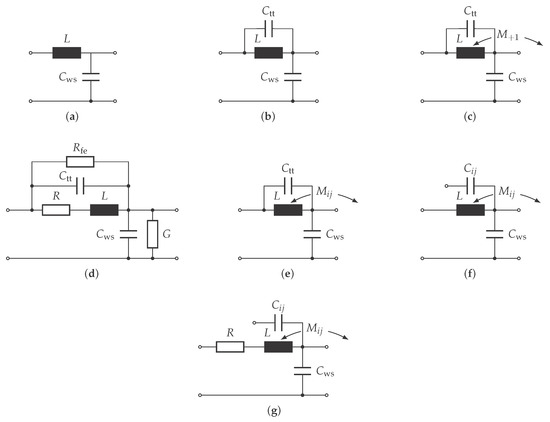
Figure 1. Chronological progression of models for the prediction of non-uniform potential distributions. (a) P. H. Thomas 1902 [3]; (b) K. W. Wagner 1915 [4], A. von Jouanne 1996 [10]; (c) R. Rüdenberg 1926 [14]; (d) L. V. Bewley 1931 [5]; (e) P. A. Abetti 1955 [6], B. C. Robinson 1953 [7]; (f) B. C. Robinson 1956 [8], M. T. Wrigth 1983 [9]; (g) O. Magdun 2016 [12], Y. Xie 2019 [11].

Note that the awareness of all necessary interactions and effects existed from the beginning (as introduced by J. C. Maxwell [15]) but was not considered due to mathematical complexity. The interactions between turns were understood by means of capacitances and inductances as distributed components. In order to simplify the underlying partial differential equations, ladder network lumped circuit elements were used. Table 1 gives a comprehensive comparison.

Table 1. Comprehensive comparison of the models and the effects which are taken into account, all models include the winding-stator capacitance.

Author	Date	Application	Turn-Turn Capacitance	Mutual Inductance	Additional Effects	Solution
P. H. Thomas	1902	Transformer	no	no	none	Non-mathematical discussion
K. W. Wagner	1915	Transformer	yes	no	none	Analytical PDE
E. W. Boehne	1930	Electrical Machines	no	no	none	Transmission line
					iron losses
L. V. Bewley	1931	Transmission Systems	yes	indirect	insulation resistance	Analytical PDE
P. A. Abetti	1953	Electrical Machines,	yes	yes	none	numerical
		Transformer
B. C. Robinson	1956	Electrical Machines	yes	yes	none	PDE system, analytical
						with simplifications
R. Rüdenberg	1962	Electrical Machines,	yes	simplified	approximate current	Analytical PDE
		Transformer			displacement
M. T. Wright	1983	Electrical Machines	yes	yes	approximate current	PDE system, numerical
					displacement	equivalent circuit
A. von Jouanne	1996	Electrical Machines	yes	no	none	Not mentioned
O. Magdun	2016	Electrical Machines	yes	simplified	approximate frequency	PDE system, numerical
					dependence for R and L	equivalent circuit
Y. Xie	2019	Electrical Machines	yes	yes	current displacement	Coupled circuit and
						mag. FEM simulation

Recent publications, such as [12], use the finite element method (FEM) to calculate the inductance matrix $\mathit{L}$ and capacitance matrix $\mathit{C}$ of a stator slot filled with conductors. The matrix identification computing effort is mostly determined by the number of conductors and requires knowledge of the conductors’ exact arrangement within the stator slot. The scope of FEM-based models is expanded in [16] to include the examination of circulating currents in an electrical machine’s winding.

With the application of FEM to identify the inductance and capacitance matrices of a slot filled with conductors comes the question about the exact placement of these conductors. While the process to build a reasonable model for form-wound windings from engineering data is straightforward, a model for random-wound windings becomes challenging. Conductor distributions are derived from cut-open electrical machines in [11,16]; they form the basis for HF investigations, but cut-open electrical machines are often unavailable. Image processing is used in recent but unpublished research to estimate the conductor positions inside the stator slot, which also relies on cut-open electrical machinery.

In order to compute realistic winding-to-stator capacitances, the authors published an article addressing the generation of realistically filled stator slots from design data by utilizing probability density functions (PDF) [17]. The same procedure is used in this publication, as it delivered promising results when compared to measurements.

Therefore, this paper presents a complete methodology to compute the non-uniform potential distribution in electrical machine windings under pulse voltage stress. Utilizing probability density functions for the generation of realistically filled stator slots, FEM is used to identify the resistance, inductance, and capacitance matrices, and numeric circuit simulation is used to solve an extensive equivalent circuit in the frequency domain.

Following this introduction, the method is described in detail and all made assumptions are discussed. Following this, results from the field simulation, the subsequent parameter identification, and the full prediction capability of the method are shown. The last section provides a conclusion as well as remarks on further research.

2. Method

This section is separated in accordance to the flowchart of the complete methodology in Figure 2 and describes the methodology in detail. Briefly, the methodology consists of the following key aspects: two different field simulations are executed. Those provide input parameters for the equivalent circuit model, which is solved in the frequency domain, and the result is multiplied with an input signal. This leads to the potential distribution of the winding in the frequency domain. After an inverse Fourier transformation, the potential distribution can be visualized and processed further.

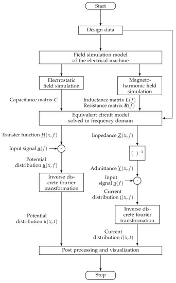
Figure 2. Flowchart of the complete methodology.

2.1. Design Data

The method starts by aggregating the necessary design data in order to prepare a model of the electrical machine. Included in this design data are the detailed geometry of the electrical machine as indicated in [1], winding and insulation properties as stated in Table 2 as well as the winding plan shown in [18].

Table 2. Winding, geometrical, and insulation properties of stator specimen S3.

Property	Value
Rated power	75 kW
Rated torque	27 Nm
No. of pole pairs	2
Rated speed	25,000 min${}^{-1}$
Max. speed	50,000 min${}^{-1}$
Stator length	110 mm
Stator outer diameter	160 mm
Stator inner diameter	82 mm
No. of stator slots	24
No. of turns per coil	5
Diameter of conductors	0.4 ... 0.6 mm
No. of parallel branches per phase	2
No. of parallel strands per turn	24
Copper fill factor	0.35
Ground wall insulation thickness	220 $\mathsf{\mu }$m
Phase-to-Phase insulation thickness	170 $\mathsf{\mu }$m
Slot wedge thickness	370 $\mathsf{\mu }$m
Stator core material	NO20-15 electrical steel

In general, it should be noted that more detailed data is beneficial, e.g., frequency-dependent material data or sectional views of the stator slots. However, missing data can be obtained by approximations, averages, or statistical distributions, and yet satisfactory results can still be achieved.

Typically, geometric data of the stator are available in form of drawings or computer-aided design (CAD) data. An important role comes to the known material properties, such as electric conductivity and relative permeability of the electrical steel sheets used for the stator, the relative permittivity of the used insulation materials, and the dimension and insulation thickness of the conductors used for the winding. As no sector-specific assumptions are made, the method can be transferred in the industrial sector.

2.2. Field Simulation Model of the Electrical Machine

In order to determine the required parameter matrices $R\left(f\right), L\left(f\right)$ and $C$, two separate field simulations are performed: electrostatic and magneto-harmonic. Each field simulation is conducted on a separate model which saves time during the computation, however, one holistic, but more complex model is sufficient. Depending on the fundamental partial differential equation to be solved, appropriate boundary conditions are selected. In cases where the location of the individual conductors inside the stator slot are unknown, a realistically filled stator slot is generated from a probability density function (PDF). This approach is discussed in [17] and applied in this publication. Other approximations that follow deterministic patterns are unsuitable for random-wound windings. Now, we follow the discussion of the electrostatic and the magneto-harmonic field simulation.

2.2.1. Electrostatic

The electrostatic field simulation is carried out for the two-dimensional model shown in Figure 3. Material properties are assigned in accordance with data provided by manufacturer’s data sheets. In this case, the ground wall insulation ${\epsilon }_{\mathrm{r}}=2.16$, the phase insulation ${\epsilon }_{\mathrm{r}}=1.93$, the turn insulation ${\epsilon }_{\mathrm{r}}=4.17$, and the slot wedges ${\epsilon }_{\mathrm{r}}=2.53$ have different relative permittivities ${\epsilon }_{\mathrm{r}}$. A turn consists of 24 parallel strands and related strands are highlighted in the same color. As there is no conductivity concept in electrostatics, all edges of the stator core and the individual conductor are imposed with equipotential boundary conditions. The model shown in Figure 3 forms the smallest repeating entity for the electrostatic field simulation.

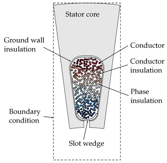
Figure 3. Two-dimensional electrostatic field simulation model.

2.2.2. Magneto-Harmonic

The magneto-harmonic field simulation is carried the on the two-dimensional model shown in Figure 4. Materials are assigned in accordance with the manufacturer’s data sheets; the specific values are given in Table 2. As shown below, the magneto-harmonic field simulation does not consider the effects of insulation materials. The insulation material is thus ignored and therefore not shown in the model. Instead of the whole winding, two coils are placed inside the slots of the stator core. These two coils form the smallest repeating entity for the magneto-harmonic field simulation. Depending on the number of pole pairs, the winding configuration, and whether a rotor is considered, specific boundary conditions may apply to reduce the model size using symmetry. As no symmetry can be found for this configuration, a full stator model is required.

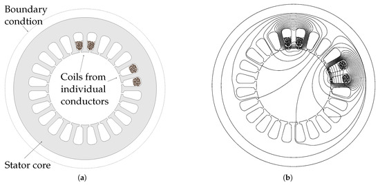
Figure 4. Model and solution for magneto-harmonic field simulation. (a) Field simulation model. (b) Magnetic field lines at $f=100$ Hz.

At this point, current displacement is only considered inside the conductors of the winding but is neglected inside the stator iron sheets. This is because the stator core is laminated along the z-axis and the two-dimensional field simulation does not allow for model discontinuities in this axis. To overcome this hurdle

1.

a complex frequency-dependent permittivity $\underline{\mu }\left(f\right)={\mu }^{\prime }\left(f\right)-\mathrm{j}{\mu }^{″}\left(f\right)$, derived from measurements, can be used during a time-harmonic field simulation;

2.

a method introduced by Kaden [19] can be applied after a linear or during a nonlinear time-harmonic field simulation. It derives a frequency-dependent effective permittivity from the relative permittivity, the specific electric conductance, and thickness of the iron sheets. The consequences of effective permeability are comparable to those of complex permeability mentioned first; or

3.

the current displacement is considered in each individual sheet and conductor by means of a three-dimensional field simulation.

From the points mentioned above, the second method was chosen, because Kaden’s method has been found valuable in other publications [12,20] and does not rely on measurements. Nevertheless, a more concrete comparison of the first two would be beneficial.

2.3. Equivalent Circuit Model

From the circuits shown in Figure 1, the single-turn model shown in Figure 5 is derived, which incorporates the following aspects:

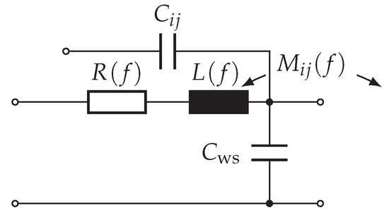
Figure 5. Single-turn model with frequency-dependent turn resistance R, self-inductance L, mutual inductance M, and frequency-independent capacitance C.

1.

frequency dependence of turn resistance $R\left(f\right)$, self-inductance $L\left(f\right)$ and mutual inductance $M\left(f\right)$, caused by current displacement in conducting material, and

2.

capacitances C between all conducting surfaces, including turns, coils, phases, and the stator core, and

3.

propagation delay due to the distributed nature of all elements mentioned above.

By connecting multiple single-turn models, every other turn-based structure can be modeled, including electrical machine stator windings. A generic multi-turn model can be represented by connecting n single-coil models in series as shown in Figure 6.

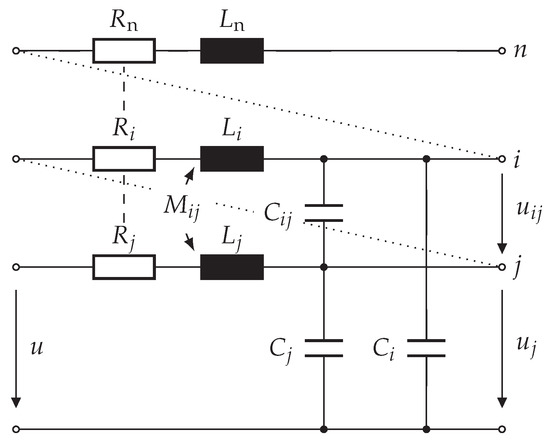
Figure 6. Multi-turn model by connecting n single-turn models in series; the circuit elements are frequency-dependent as shown in Figure 5, and all turns including the nth-turn share mutual inductive and capacitive couplings (not drawn).

The representation is relatable to the multi-conductor transmission line model presented by C. R. Paul in [21] with the addition, that the end of a turn is the beginning of the next turn until all turns are considered. This turn-to-turn connection is illustrated by diagonal dotted lines, while vertical dashed lines represent the repetition of the single-turn model. The voltage $u_j$ is the voltage between the jth turn and the reference conductor, the voltage $u_{i,j}$ is the voltage between the ith and the jth turn, and the voltage u is the voltage applied between the model beginning (first turn) and the reference conductor.

Under certain conditions, a turn-based model is insufficient. This is especially the case, when the maximum frequency of interest is high and the electrical machine is large. Therefore, the single-turn model and subsequently the multi-turn model can be subdivided further into k circuits. Such subdivision is known from the approximation of distributed circuits and transmission lines [21]. An example is given in Figure 7, where the multi-turn model indicated in Figure 6 is subdivided into k circuits.

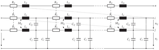
Figure 7. Distributed multi-turn model after subdividing each turn of the multi-turn model in Figure 6, same as in the multi-turn model, the circuit elements are frequency-dependent and all turns including the nth-turn share mutual inductive and capacitive coupling (not drawn).

The circuit elements are weighted in accordance with the number of divisions k to maintain the net properties of an undivided multi-turn model. The result is a frequency-dependent model which can be scaled depending on the frequency of interest and is applicable to form-wound and to random-wound windings.

2.4. Implementation

The model is strictly solved in the frequency domain, which simplifies the computation. This advantage is particularly relevant because the strong frequency dependence can be directly taken into account. Furthermore, the solution process can be parallelized as indicated in Figure 8.

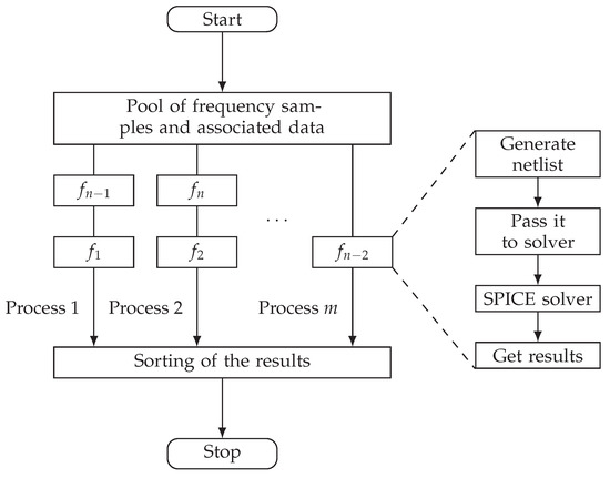
Figure 8. Asynchronous multiprocessing of n tasks in the frequency domain by m processes and recombination of the results.

This is achieved by creating a pool, in which each frequency of interest is associated with its sample of the frequency-dependent data. Then, a number of m processes executes the given instruction asynchronously on the data given in the pool. The instructions are as follows: First, a SPICE-readable net-based netlist is generated, which contains all necessary information. Then, the netlist is passed to the SPICE solver, which, after successfully finding the solution, returns the result.

After all results are available, they are sorted to yield the transfer function H and the impedance Z, which are both frequency- and spatially-dependent. These two quantities contain all the information from the linear passive model presented earlier and form the basis for the results in the following section.

3. Results and Discussion

This section will present the results and point out limitations of the methodology described in Section 2. Shown and compared with measurements, when possible, are the field simulation results, the evaluation of the equivalent circuit and the final potential distribution. The stator specimen S3 is shown in Figure 9 in a fixture for high-frequency measurements. Through high-frequency connectors, the winding terminals and a limited number of individual turns can be accessed. In [1] a full overview of the measuring process and setup is given. Frequency-dependent resistance and inductance measurements are derived from impedance measurements taken with an Omicron Bode 100 Network Analyzer on the same setup.

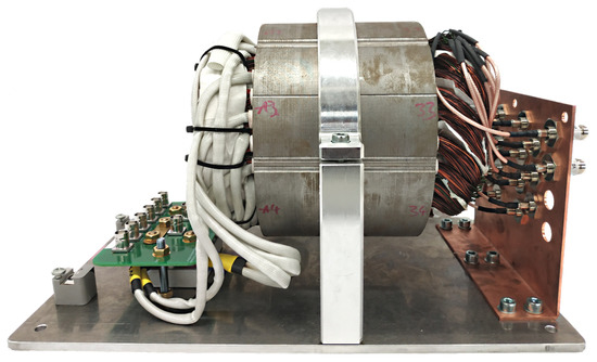
Figure 9. Electrical steel stator specimen S3 with three-phase winding and terminal board on the left side and inter-winding terminals on the right. This fixture’s base measurements are 300 mm by 230 mm.

3.1. Field Simulation

Figure 10 shows the magneto-harmonic field simulation results for turn resistance, turn inductance, and the inductive coupling coefficient on a turn-to-turn basis.

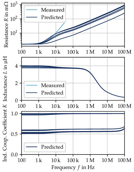
Figure 10. Magneto-harmonic field simulation results for turn resistance, turn inductance, and the inductive coupling coefficient on a turn-to-turn basis.

For the turn resistance, it can be observed that the measurement and the result of the field simulation disperse towards higher frequencies. As the comparison is made on a double logarithmic scale, both results have an exponential relationship with regard to frequency. Therefore, the absolute difference is significant and must be given further consideration. Under the applied circumstances in the field simulation, current displacement inside the stator iron sheets is not taken into account. This is common procedure in transient operating point simulations, as the thickness of the iron sheets d is much smaller compared to the equivalent conductor surface (skin depth) $\delta$. Kaden [19] derived $d<2\delta$ as approximation for which an equal field distribution inside the iron can be assumed, and $d>2\delta$ for the approximation that the field is distributed in a thin layer along the edges. The layer width is in the order of magnitude of the equivalent conductor surface $\delta$. A cutoff frequency has been introduced by Wolman [22], the effective permeability cutoff frequency

$$f_{\mu }=\frac{4}{\pi d^2\mu \kappa },$$

(1)

by setting the transition between equal and unequal field distribution at $d=2\delta$. Applying this approximation to the used stator core yields $f_{\mu }<15$ kHz, which is significantly lower than the highest frequency of interest. Therefore, current displacement in the stator iron sheets should be taken into account.

The turn inductance shows a satisfactory agreement with the measurement. However, it would be interesting to validate the prediction at higher frequencies. However, no measurement method is known for this, since the capacitive behavior of the stator towards high frequencies is dominant. As stated in Section 2.2.2, the turn inductance accounts for the formation of eddy currents inside the stator iron sheets. The sudden drop in inductance on the logarithmic scale indicates the consideration.

The inductive coupling coefficient

$$K=\sqrt{\frac{M_{ij}}{L_{ii}{L}_{jj}}}$$

(2)

between two turn inductances $L_{i,i}$ and $L_{j,j}$ with their mutual inductance $M_{i,j}$ remains steady up to shortly before the end of the considered frequency range. It does not consider the effect of eddy currents inside the stator iron sheets. Deviations of the inductive coupling coefficient are explained by their relative positions within the stator slots and the stator slots themselves. Inductive coupling within a stator slot is on an average at 0.98 and at 0.6 between stator slots belonging to a coil. Towards higher frequencies, the inductive coupling coefficient starts to increase. This cannot be explained physically and tends to be a result of an insufficient discretization during the field simulation.

The results of the electrostatic simulation are compared to a capacitive measurement of the winding. Therefore, the net capacitance

$$C_{\mathrm{ws}}=N_1\sum _{i=1}^m\sum _{j=1}^m{C}_{ij}$$

(3)

between all conductors inside a slot and the stator core is calculated and multiplied by the number of stator slots $N_1$. This yields a value for the winding-to-stator capacitance which can be measured. The measured winding-to-stator capacitance ${\widehat{C}}_{\mathrm{ws}}=2.67$ nF and the predicted capacitance $C_{\mathrm{ws}}=2.66$ nF leave a negligibly small absolute error. Details on the measurement of the winding-to-stator capacitance are given in [1,18] and on the prediction using PDF in [17].

3.2. Impedance and Transfer Function

After solving the equivalent circuit in the frequency domain, the transfer function $\underline{H}(x,f)$ and the impedance $\underline{Z}(x,f)$ are obtained. Both are frequency- and spatially-dependent. The spatial dependence x refers to the individual turns of the winding. This means that

$$\underline{H}(x,f)=\frac{{\underline{u}}_n(x,f)}{\underline{u}\left(f\right)}$$

(4)

represents the relationship between the voltage at the electrical machine’s terminals $\underline{u}\left(f\right)$ and the voltage at the end of a turn or at the beginning of the next turn ${\underline{u}}_n(x,f)$, (see Figure 6). Figure 11 shows the absolute value and the phase angle of the predicted and measured impedance.

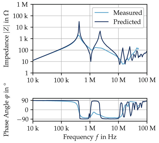
Figure 11. Measured and predicted impedance of S3 and inter-winding resonances.

For the resonance and anti-resonance frequencies, there is a good agreement between prediction and measurement. Disagreement can be observed for the absolute value and the phase angle at those frequencies. As the equivalent circuit tends to underestimate at resonances and to overestimate at anti-resonances, a lack of dissipative elements inside the equivalent circuit is concluded. Considered, and already acting, as dissipative element is the turn resistance R. However, viewed from a physical perspective, there are more effects taking place. Additional to the frequency-dependent turn resistance,

1.

a changing magnetic field inside the stator core causes losses, these being represented by a resistance parallel to the inductance L and accounting for all three types of magnetic losses (eddy current, hysteresis and excess);

2.

a time-varying electric field inside a dielectric material, like conductor insulation, slot insulation and phase insulation (Figure 3), causes dielectric losses, which are represented by a resistance in series (equivalent circuit resistance) with the related capacitance; or

3.

a conductance parallel to a capacitance in order to account for conduction losses caused by leakage currents through the dielectric, compared to the loss mechanisms mentioned above; this is the least significant,

can be incorporated to the model indicated in Figure 5. This results in the model indicated in Figure 12, where all resistances are frequency-dependent and would greatly improve the model’s capability to reflect the underlying physics. However, determining those elements requires further measurements on material samples.

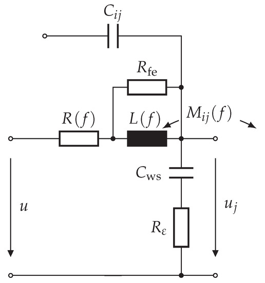
Figure 12. Single-turn model with frequency-dependent turn resistance R, self-inductance L, mutual inductance M, frequency-independent capacitance C and the additional loss elements $R_{\mathrm{fe}}$ for iron losses and $R_{\epsilon }$ for dielectric losses.

3.3. Potential Distribution

As the transfer function $\underline{H}(x,f)$ represents the relationship between the voltage at the electrical machine’s terminals $\underline{u}\left(f\right)$ and the voltage at the end of a turn or at the beginning of the next turn ${\underline{u}}_n(x,f)$, the frequency domain potential distribution is given by

$$\underline{u}(x,f)=\underline{u}\left(f\right)\underline{H}(x,f),$$

(5)

where $\underline{u}\left(f\right)$ is the terminal voltage in the frequency domain. Transformations between time domain and frequency domain are performed by the complex Fourier transformation, and vice versa, by the inverse complex Fourier transformation. However, because the calculation is numerical, the discrete Fourier transformation implemented [23,24] in Python NumPy is used.

Figure 13 shows the resulting turn-to-ground voltages of the first ten turns. The oscillations that occur can be assigned to the resonances of the differential mode impedance indicated in Figure 11. The inter-winding behavior, and thus the potential difference between the turns, is dominated by the second oscillation. It dominates the propagation characteristic of the stator winding and directly impacts the potential distribution. When iron losses and dielectric losses are not taken into account, the resonances will be inappropriately damped. Nevertheless, findings can be made about the voltages between the turns. Figure 14 indicates the voltage difference between the first and the tenth turn.

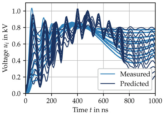
Figure 13. Turn-to-ground voltages for the first ten turns of stator specimen S3, measured and predicted, with an input voltage gradient $\mathrm{d}u/\mathrm{d}t=30$ V/ns.

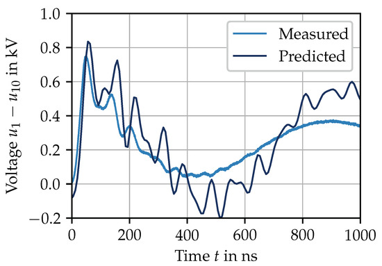
Figure 14. Voltage difference over the first ten turns of stator specimen S3, measured and predicted.

A solid agreement between measurement and prediction can be seen. The occurring oscillations also translate into the prediction of the voltage difference in a trending manner consistent with the measurement. The voltage difference between the first and the tenth turn reaches a level close to the dc-link voltage shortly after the voltage pulse is applied. The reasons for this are

1.

the oscillation of the applied pulse at the terminals causing it to exceed the dc-link voltage (overshoot) and

2.

the propagation time of the voltage pulse being longer than its rise time.

While the first argument is mainly caused by the parasitic properties of the voltage source inverter or cable, the second argument relies on the properties of the stator itself. It may therefore be appropriate to derive a stator specific-property, valid for high frequencies, that enables the findings to be applicable in a broader way. Note that if no additional manufacturing steps are applied, the initial and last turns of a coil may be close together. The stator specimen under investigation has a two-layer winding with ten turns per coil and two slots per pole and phase. However, there is no further insulation in the end winding, allowing direct contact between the first and tenth turns of a coil.

Finally, the potential distribution is presented in Figure 15.

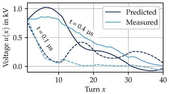
Figure 15. Potential distribution for stator specimen S3 at different points in time, measured and predicted.

Prediction and measurement are slightly in line due the oscillations. The cause and effect of the oscillations were addressed before and improvements to the model were proposed. Figure 15 shows that the turn-to-ground voltage not only exceeds the dc-link voltage at the motor terminals but also inside the stator winding. The exceedance can be seen between position $x=5$ and $x=8$ at $t=0.4$ µs. Therefore, the insulation of certain turns is more stressed.

As this behavior of the stator winding is neither measurable nor predictable by non-distributed models, it poses a novel finding in the context of the high-frequency analysis of electrical machines. Stator windings, where the inter-winding frequency is slightly damped and excited by a voltage pulse, are particularly affected.

4. Conclusions

The methodology presented is capable of predicting the impedance of an electrical machine over a wide frequency range. As, apart from the winding resistance, no other lossy elements are taken into account, oscillations occur. Those oscillations are also observed in the measurement but they are damped due to losses. An alternative single-turn model is presented in Figure 12, which incorporates iron and dielectric losses through additional resistances. Although the basic problem is an electromagnetic field problem, it can be approximated as an equivalent circuit model to get good results. Two key findings are made: First, additional voltage stress between adjacent turns occurs due to the propagation of the voltage pulse through the winding, and second, additional voltage stress is imposed between turns and the stator core. As stated, material measurements, both for the stator core and the insulation materials, are necessary. From these values for the lossy elements can be derived and the dampening effect can taken into account. As the oscillations are a key part of the observations, the intentional use of lossy insulation material in order to invoke additional damping will be investigated in the future.

Additional insulation of the first coil or the first few turns can also help to reduce voltage stress. More research is needed to determine whether the added voltage stress is dependent on the voltage gradient $\mathrm{d}u/\mathrm{d}t$, whether partial discharges occur, and how these findings might be applied to electrical machine lifetime prediction.

References

- Hoffmann, A.; Ponick, B. Method for the Prediction of the Potential Distribution in Electrical Machine Windings under Pulse Voltage Stress. IEEE Trans. Energy Convers. 2020, 36, 1180–1187. [Google Scholar] [CrossRef]
- Boehne, E.W. Voltage Oscillations in Armature Windings under Lightning Impulses-I. Trans. Am. Inst. Electr. Eng. 1930, 49, 1587–1607. [Google Scholar] [CrossRef]
- Thomas, P.H. Static Strains in High Tension Circuits and the Protection of Apparatus. Trans. Am. Inst. Electr. Eng. 1902, XIX, 213–264. [Google Scholar] [CrossRef]
- Wagner, K.W. Das Eindringen Einer Elektromagnetischen Welle in Eine Spule Mit Windungskapazität. Elektrotechnik Und Maschinenbau 1915, 33, 89–92. [Google Scholar]
- Bewley, L.V. Transient Oscillations in Distributed Circuits With Special Reference to Transformer Windings. Trans. Am. Inst. Electr. Eng. 1931, 50, 1215–1233. [Google Scholar] [CrossRef]
- Abetti, P.A.; Adams, G.E.; Maginniss, F.J. Oscillations of Coupled Windings [Includes Discussion]. Trans. Am. Inst. Electr. Eng. Part III Power Appar. Syst. 1955, 74, 12–21. [Google Scholar] [CrossRef]
- Robinson, B. The Propagation of Surge Voltages through High-Speed Turbo-Alternators with Single-Conductor Windings. Proc. IEE-Part II Power Eng. 1953, 100, 453–467. [Google Scholar] [CrossRef]
- Robinson, B. The Propagation of Surge Voltages through Turbo-Alternators with Concentric-Conductor-Type Windings. Proc. IEE Part A Power Eng. 1956, 103, 355. [Google Scholar] [CrossRef]
- Wright, M.; Yang, S.; McLeay, K. General Theory of Fast-Fronted Interturn Voltage Distribution in Electrical Machine Windings. IEE Proc. B Electr. Power Appl. 1983, 130, 245. [Google Scholar] [CrossRef]
- Von Jouanne, A.; Enjeti, P.; Gray, W. Application Issues for PWM Adjustable Speed AC Motor Drives. IEEE Ind. Appl. Mag. 1996, 2, 10–18. [Google Scholar] [CrossRef]
- Xie, Y.; Zhang, J.; Leonardi, F.; Munoz, A.; Degner, M.; Liang, F. Voltage Stress Modeling and Measurement for Random-Wound Machine Windings Driven by Inverters. IEEE Trans. Ind. Appl. 2020, 56, 3536–3548. [Google Scholar] [CrossRef]
- Magdun, O.; Blatt, S.; Binder, A. Calculation of Stator Winding Parameters to Predict the Voltage Distributions in Inverter Fed AC Machines. In Proceedings of the 2013 9th IEEE International Symposium on Diagnostics for Electric Machines, Power Electronics and Drives (SDEMPED), Valencia, Spain, 27–30 August 2013; IEEE: Piscataway, NJ, USA, 2013; pp. 447–453. [Google Scholar] [CrossRef]
- Sundeep, S.; Wang, J.; Griffo, A.; Alvarez-Gonzalez, F. Antiresonance Phenomenon and Peak Voltage Stress Within PWM Inverter Fed Stator Winding. IEEE Trans. Ind. Electron. 2021, 68, 11826–11836. [Google Scholar] [CrossRef]
- Rüdenberg, R. Elektrische Wanderwellen auf Leitungen und in Wicklungen von Starkstromanlagen; Springer: Berlin, Germany, 1962. [Google Scholar]
- Maxwell, J.C. A Treatise on Electricity and Magnetism; Cambridge University Press: Cambridge, UK, 2010. [Google Scholar]
- Xie, Y.; Zhang, J.; Leonardi, F.; Munoz, A.R.; Degner, M.W.; Liang, F. Modeling and Verification of Electrical Stress in Inverter-Driven Electric Machine Windings. IEEE Trans. Ind. Appl. 2019, 55, 5818–5829. [Google Scholar] [CrossRef]
- Hoffmann, A.; Knebusch, B.; Stockbrugger, J.O.; Dittmann, J.; Ponick, B. High-Frequency Analysis of Electrical Machines Using Probability Density Functions for an Automated Conductor Placement of Random-Wound Windings. In Proceedings of the 2021 IEEE International Electric Machines & Drives Conference (IEMDC), Hartford, CT, USA, 17–20 May 2021; IEEE: Piscataway, NJ, USA, 2021; pp. 1–7. [Google Scholar] [CrossRef]
- Hoffmann, A.; Ponick, B. Statistical Deviation of High-Frequency Lumped Model Parameters for Stator Windings in Three-Phase Electrical Machines. In Proceedings of the 2020 International Symposium on Power Electronics, Electrical Drives, Automation and Motion (SPEEDAM), Sorrento, Italy, 24–26 June 2020; IEEE: Piscataway, NJ, USA, 2020; pp. 85–90. [Google Scholar] [CrossRef]
- Kaden, H. Wirbelströme und Schirmung in der Nachrichtentechnik; Springer: Berlin/Heidelberg, Germany, 1959. [Google Scholar] [CrossRef]
- Muetze, A. Bearing Currents in Inverter-Fed AC-Motors; Shaker-Verlag GmbH: Düren, Germany, 2004. [Google Scholar]
- Paul, C.R. Analysis of Multiconductor Transmission Lines, 2nd ed.; Wiley-IEEE Press: Hoboken, NJ, USA, 2007. [Google Scholar]
- Wolman, W. Influence of Eddy Current in Transmitting Sheets as Function of Frequency, Der Frequenzgang Des Wirbelstromeinflusses Bei Uebertragerblechen. Z. Fuer Tech. Phys. 1929, 10, 595–598. [Google Scholar]
- Cooley, J.W.; Tukey, J.W. An Algorithm for the Machine Calculation of Complex Fourier Series. Math. Comput. 1965, 19, 297–301. [Google Scholar]
- Press, W.H. (Ed.) Numerical Recipes: The Art of Scientific Computing, 3rd ed.; Cambridge University Press: Cambridge, UK; New York, NY, USA, 2007. [Google Scholar]
Publisher’s Note: MDPI stays neutral with regard to jurisdictional claims in published maps and institutional affiliations. |
© 2022 by the authors. Licensee MDPI, Basel, Switzerland. This article is an open access article distributed under the terms and conditions of the Creative Commons Attribution (CC BY) license (https://creativecommons.org/licenses/by/4.0/).