Natural Gas Consumption Forecasting Based on the Variability of External Meteorological Factors Using Machine Learning Algorithms

Abstract

Natural gas consumption depends on many factors. Some of them, such as weather conditions or historical demand, can be accurately measured. The authors, based on the collected data, performed the modeling of temporary and future natural gas consumption by municipal consumers in one of the medium-sized cities in Poland. For this purpose, the machine learning algorithms, neural networks and two regression algorithms, MLR and Random Forest were used. Several variants of forecasting the demand for natural gas, with different lengths of the forecast horizon are presented and compared in this research. The results obtained using the MLR, Random Forest, and DNN algorithms show that for the tested input data, the best algorithm for predicting the demand for natural gas is RF. The differences in accuracy of prediction between algorithms were not significant. The research shows the differences in the impact of factors that create the demand for natural gas, as well as the accuracy of the prediction for each algorithm used, for each time horizon.

1. Introduction

1.1. The Importance of Natural Gas Demand Prediction

Natural gas is one of the most important sources of energy. Generation of 1 MJ of energy from it produces the lowest amount of CO₂ among all fossil fuels [1]. Relatively easy distribution and storage determines its safe use. It is seen as the so-called transition fuel that will help to bring about the energy transition in developed countries [2]. In Poland, the use of natural gas in industry, e.g., for heating purposes or in technological processes, is cheaper and more environmentally friendly than the use of electricity produced mainly from coal for these purposes. The energy market is not indifferent to these properties of “blue fuel”.

In Poland the consumption of natural gas is close to 20 billion m3 per year. Deliveries of this fuel have been diversified in recent years. Currently the main sources of natural gas for Poland are Russia (via pipelines) and Qatar, USA, and Norway (via LNG terminal) and own resources (approx. 20%). In 2022, the Baltic Pipe gas pipeline will be launched, which will reduce supplies from Russia while supplies from Norway and Denmark will increase. The progressive increase in demand for natural gas, estimated in Poland at about 23 billion m³ in 2030 [3], brings with it a number of challenges. The share of gas in the structure of primary energy consumption increased from 8.5% (1990) to 13.4% (2011) [4] and 15% in 2018 [5]. Most European countries import this source through the system of gas pipelines connected to countries with natural gas resources, relying on a lesser extent on domestic production [6]. Some European Union countries also use LNG terminals to increase natural gas supplies to diversify their sources [7].

The end user most often receives natural gas from the distribution network. The design assumptions of each element of the gas system must be adequate to the planned demand. Natural gas consumption forecasts for the coming years are included in the design process [8].

Knowing the exact demand for natural gas is essential for the smooth, efficient and economically viable use of natural gas by end-users [9]. A number of methods have been developed for this purpose, which have been reviewed by Soldo [8] and other authors [10].

1.2. Methods of Forecasting Natural Gas Demand Literature Overview

Natural gas consumption by consumers varies over time, although on the basis of the analyzed data certain cycles can be noticed, both daily, weekly, and annually. Currently in Poland the coincidence factor is used as the dominant approach for forecasting the NG demand across municipal customers. Its calculation is based on quantity and type of natural gas devices in the analyzed zone. It also depends on the historical characteristics of the natural gas consumption. Additionally, it includes a simplification consisting in the unification of, for instance, the thermal insulation of buildings or the maximum power of heating devices of different types [11].

General energy demand forecasting can be based on two different types of models that have practical application. These are time models (time series) and regression models [12]. The input data used for forecasting can describe various aspects of human activity and external factors such as the weather. Time series forecasting is based on the analysis of historical data itself, using, e.g., indicators such as moving average (MA) or ARMAX, which was used in Demirel’s research [12]. Erdogdu proposed to implement the ARIMA model to predict annual or monthly demand, based on factors describing the economic situation, such as GDP and gas prices [13]. Extending the input data set based on a series of variables describing the weather data, Taşpınar used the SARIMAX model to predict the daily demand in one of the Turkish provinces [14]. This model took into account the occurrence of certain cyclical changes, which improved its accuracy in relation to the ARIMAX model [15]. Although, the research of Adebiyi et al. shows that in time-series prediction, neural networks have better accuracy with reasonable performance [16].

Regression models seem to be a more advanced and accurate tool for determining gas demand. Geem implemented a linear regression model based on four economic factors—GDP, population size, and the value of exports and imports in South Korea [17]. In Bianco’s research, in addition to economic factors, the relationship between gas consumption and temperature was included for long-term gas demand forecasting [18]. In the work of Gregory D. Merkel, apart from the neural network model, a linear regression model was implemented and compared [19].

Artificial neural networks, especially the so-called Deep Neural Network (DNN) consist of a large number of neurons and layers. Their science uses the back propagation (BP) algorithm, adjusting the weight values in individual neurons. They are used to solve many regression problems, i.e., where the prediction is for continuous values, such as the amount of natural gas consumption [20]. Their possible implementation in this type of solution has been studied for at least several years. In the article by Alirez Khotanzad, artificial neural networks (ANNs) were used to predict the demand for natural gas, analysing the nonlinear dependence of natural gas demand and temperature [21,22]. These models are based on the processing of large amounts of data on which the volume of gas demand depends, as in the work of Ioannis P. Papakidis [23]. These include weather factors that affect the heating of households, such as the ambient temperature and wind speed, used in the work of Haydar Aras [24], or Gregory D. Merkel [19], which has been additionally expanded with data describing historical consumption. In the work of Feng Yu, in addition to the standard BP algorithm, optimized algorithms such as CCMGA-BP were implemented, which improved the prediction performance [22]. The alternative approach to the problem is the usage of multi-level genetic programming, as it was shown in the research by Forouzanfar et al. [25]. Genetic algorithms can be helpful in building simple models used for prediction, which have a good accuracy-performance ratio [26]. Although, this paper is focused more on the regression approach.

It should be noted that machine learning methods can enhance the natural gas industry in many sectors. First of all, the use of machine learning, in addition to the NG consumption prediction discussed in this article and many other papers [27,28,29], is possible in the case of the possibility of detecting hydrates formation [30], predicting changes in natural gas prices on energy markets [31,32], locating gas network leaks [33] and others.

1.3. Approach Presented in Article

An important factor influencing the diversification of the hourly and daily consumption is the activity of the society related to, inter alia, cooking, water heating or various types of industrial and heating processes [11], which were included in the presented research. Additionally, it was extended by checking the use of the Random Forest Regression algorithm in solving the problem of determining the demand for natural gas.

Knowing the amount of natural gas consumption, understood as the load on the gas network, is crucial in regard to simulating the gas network and managing the gas flow in the network [11]. The share of municipal consumers in the shaping of the gas consumption structure in Poland is approx. 28% [34]. In addition, the implementation of this type of technology in common use would bring a number of other benefits and would be in line with the current energy policy of the European Union [35]. The proposed solution in this paper provides better possibilities than the currently used model-based methods and operates on a more weather-based data set. That approach is connected to the varied weather conditions in Poland over the year. In this paper, the possibilities of forecasting the natural gas demand are tested in a climate with six thermal seasons, with relatively hot summers and cold winters. By using the weather stations network it is scalable and potentially can be easily implemented in a nationwide scale.

In summary, the main goals of this article are:

• Proving that with different climate it is possible to accurately forecast the demand for natural gas among municipal consumers;
• Determining which factors have a significant impact on the demand for natural gas;
• Comparing the three different models used for the forecast.

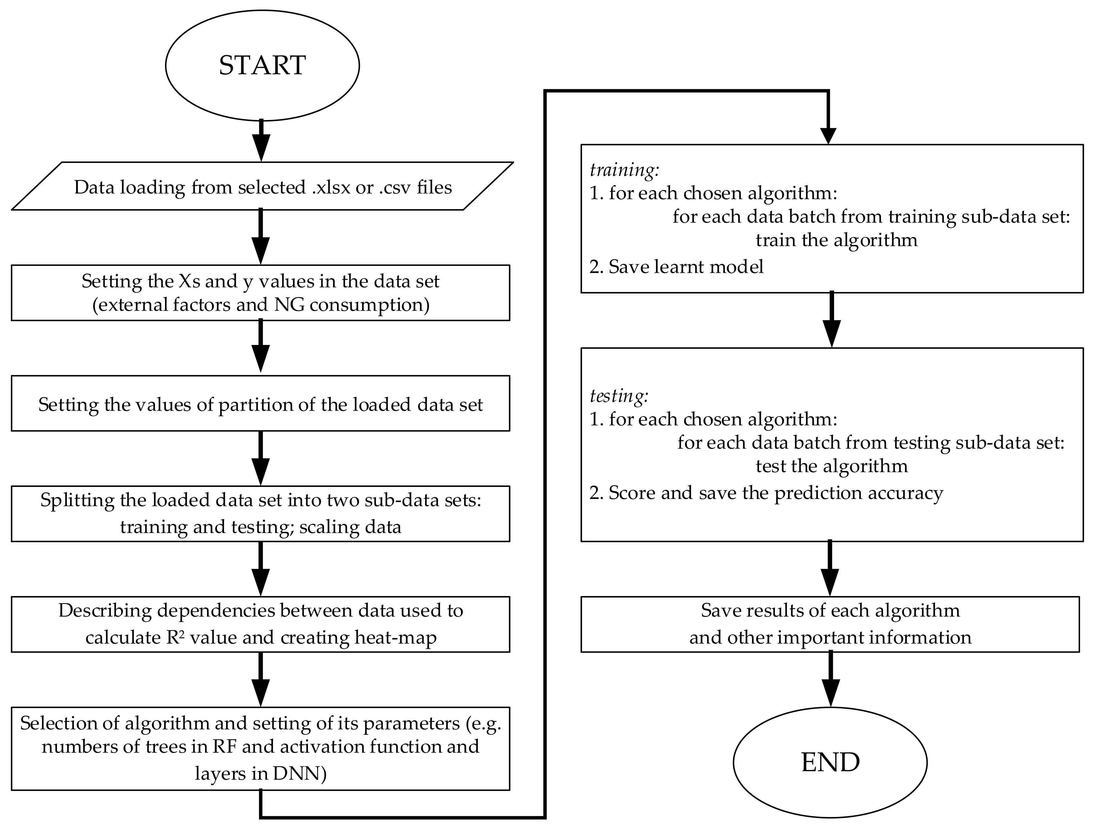
2. Methods

In the presented work, three types of machine learning algorithms, Multiple Linear Regression (MLR), Random Forest (RF) and Deep Neural Network (DNN) are compared [36]. The considered problem is a typical regression problem, i.e., one whose purpose is to predict the value of the variable $Y$, depending on the values of the variables describing $X$ [20,37]. In the study, variable $Y$ was gas consumption, and variables $X$ were data describing external factors such as weather components and historical gas consumption.

Natural gas forecasting methods were selected on the basis of publications on similar issues. They seem to be prospective in terms of accuracy and ease of implementation on a larger scale.

The first regression model used in the presented research was Multiple Linear Regression. Despite the fact that it is one of the simplest statistical methods, it can be used to solve complex problems such as forecasting the demand for natural gas, which was shown, among others, in the works of Merkel, Bianco and Geem [17,18,19].

From a mathematical point of view, its operation can be reduced to a simple equation in which the predicted value depends on the sum of the product of independent variables and their weights and the intercept b₀ (regression intercept). The values of the b_n coefficients (predictors) are calculated based on the smallest squared error of the sample.

The general formula for the MLR can be written as follows:

$$\widehat{Y_i}=b_0+b_1{X}_{i1}+b_2{X}_{i2}+\dots +b_n{X}_{in}$$

(1)

The formula describing the actual (observed) value:

$$Y_i=b_0+b_1{X}_{i1}+b_2{X}_{i2}+\dots +b_n{X}_{in}+e_i$$

(2)

where:

$Y_i$ is the actual (observed) value.

$X_{i1 }\mathrm{and} X_{in}$ are the labelled data.

$b_1 \mathrm{and} b_n$ are the partial regression coefficients.

$b_0$ is the slope.

$e_i$ is the difference between real and predicted value:

$$e_i=Y_i – \widehat{Y_i}$$

(3)

Values of coefficients b are chosen in the way that the sum of squared differences between the predicted value and the actual value is as small as possible [38,39]:

$${{\displaystyle \sum }}_{i=1}^n{e}_i^2=\frac{1}{n}{{\displaystyle \sum }}_{i=1}^n{(Y_i-{\widehat{Y}}_i)}^2=min$$

(4)

Another algorithm used to predict gas demand was the algorithm “Random Forest”. It is suitable for solving regression problems such as quantitative rather than qualitative (classification) prediction. Its operation is based on creating and teaching a large collection of correlated data sets of decision trees, forests. The variables used for the creation of a tree are delivered through the bootstrap aggregation or bagging. Each individual tree consists of a series of generated decision rules which, depending on the value of the input variables, assign them to appropriate, disjoint areas. The result of the prediction is the arithmetic mean of the explained variable in the area to which it was assigned by the tree, based on the generated rules. When predicting continuous values, the number of areas should be large to minimize the number of variables explained in individual areas.

The algorithm can be described as follows:

For b = 1 to B Trees:

Select a bootstrap sample of size N from the training data set.

Grow a random-forest tree, based on the selected data:

-

Select m variables randomly from the p variables;

-

Pick the best variable/split-point among the m;

-

Split the node into two nodes;

-

Recursively repeat the last three steps for each terminal node of the tree, until the set minimum node size n_min is reached.

Output the ensemble of trees T_b^B₁.

The output of algorithm prediction in regression problems, for new point x is:

$$f_{rf}^{-B}\left(x\right)=\frac{1}{B}{\displaystyle \sum }_{n=1}^B{T}_b\left(x\right)$$

(5)

In order to improve the efficiency of the algorithm and make it less sensitive to poor quality data, whole groups of trees, Random Forests, are used. The result of the prediction is the average value of individual trees. It is an algorithm that allows you to efficiently and accurately predict continuous values [40,41,42].

In presented work, in addition to regression algorithms, a neural network was used to estimate gas demand. In the course of presented research, five topological variants were created and tested with different settings, such as activation functions. The best network was found to have 11 hidden layers. It used the ReLu activation function and the linear function, as well as the Adam optimizer, while learning the Mean Square Error. Similar networks were used in research in similar papers [19,22,43]. Schematic representation of the work of a single neuron is presented in Figure 1.

Equation describing the operation of the summation block:

$$\phi ={\displaystyle \sum }_{i=1}^n{u}_i{w}_i$$

(6)

where:

$n$ is the number of inputs.

$u_i$ is the input value.

$w_i$ is the weight.

The equation of the ReLu activation function is as follows:

$$y\left(x\right)=\{ x for x\ge 0; 0 for x<0$$

(7)

The general principle of operation of a neural network is based on the processing of input signals. Each neuron in the network receives a signal from the previous layer, with the appropriate weight. Summing up the value of the incoming signal, it transmits the value determined by the activation function (Figure 1). The supervised learning was used to solve a considered problem. In the process of learning, the algorithm received a set of data pairs, external factors and the corresponding values of natural gas consumption. While learning the network, the weights were initially selected randomly using the back propagation (BP) algorithm. They were determined in accordance with the learning vectors to minimize the loss function value between the value predicted by the network and the actual value. In this performed analysis, the loss function was the mean square error, and the activation function was the ReLu function [22,44,45,46].

For description and comparing the results of prediction, three indicators were calculated, coefficient of determination R², Root Mean Square Error (RMSE), and Mean Absolute Percentage Error (MAPE). These methods were chosen based on research of similar issues [15,19,23].

The coefficient of determination R² may be written as [47]:

$$R^2=1-\frac{{{\displaystyle \sum }}_{t=1}^n{\left(y_t-x_t\right)}^2}{{{\displaystyle \sum }}_{t=1}^n{\left(y_t-\overline{y}\right)}^2}$$

(8)

RMSE is defined with a following formula:

$$\mathrm{RMSE}=\sqrt{\frac{1}{n} {\displaystyle \sum }_{t=1}^n{\left(x_t-y_t\right)}^2}$$

(9)

and MAPE can be written as:

$$\mathrm{MAPE}=\frac{1}{n} {\displaystyle \sum }_{t=1}^n\left|\frac{x_t-y_t}{y_t}\right| ·100\%$$

(10)

where:

$n$ is the size of the sample.

$x_t$ is the predicted value.

$y_t$ is the observed value.

$\overline{y}$ is the mean of $y_t$ values.

3. Assumptions

In the presented research, the analysis of forecasting the demand for natural gas was carried out on the basis of data describing the gas flow in a five-year period at four natural gas reducing and metering stations supplying approx. 85 thousand cities in south-eastern Poland (Lesser Poland Region) (Figure 2). Detailed data on gas consumption provided by natural gas distribution operators are not a public data and cannot be directly presented in the article.

Moreover, the complete meteorological data set from at least 30 years is available for the chosen city. Additionally, the gasification level of the analysed data collected for this city used in the analysis area is significant (about 90%) [48]. This leads to the possibility of assuming that the number of municipal consumers in a given area will not change significantly over time and the cyclicality of several years caused by annual changes in the weather will not be significantly disturbed for the benefit of new consumers. In addition, there are no large industrial customers, which are connected to the mentioned distribution gas network, so the structure of demand is created mostly by the municipal customers.

The structure of natural gas consumption in the analyzed region, both daily and annual, is typical for this region of Poland, the highest gas consumption falls in the winter months, while in the summer it is very limited. In daily terms, the highest gas consumption occurs in the morning and evening hours and is associated with activities such as cooking on gas stoves or heating water [11]. This dependence showing the average hourly gas consumption in summer and winter seasons is shown in Figure 3.

4. Types of External Factors

4.1. Meteorological Factors

The performed research examined the impact of individual meteorological parameters variability on the level of natural gas consumption. Values of the Pearson correlation coefficient for individual data types and daily consumption are presented in

Table 1. Pearson correlation coefficient for individual data types and daily consumption.

Factor:	The Value of the Pearson Correlation Coefficient for the Daily Consumption and:
1	Month	0.69
2	Cloud cover	−0.035
3	Wind velocity	0.16
4	Vapor Pres.	0.19
5	Air Temperature	−0.91
6	Humidity	0.44
7	Atmospheric Pressure	0.11
8	Related Atmospheric Pressure	0.21
9	Rain/Snowfall	−0.12
10	Volume of NG in time t = −1 day	0.98
11	Day of week	0.15
X	Volume of NG demand	1

.

Additionally, the heatmap with the Pearson correlation coefficient values depending on each used variable was performed (Figure 4). For better visualization, they were labeled with numbers, used in Table 1. Natural gas consumption was the variable marked as X.

As in the works of Merkel et al., 2018; Taylor, 1990; and McKelvey and Zavoina, 2010, there is a strong correlation between the air temperature and the demand for natural gas [19,48,49]. The less significant relationship between consumption and wind speed than in the case of work [24] is most likely due to a different type of climate in Turkey than in Poland.

As shown in Figure 5, the system of points is close to linear only to a certain extent. Above a temperature of approx. 15 °C, gas consumption is constant, and as the temperature drops below approx. 15 °C, a directly proportional increase in the value of gas consumption begins. After reaching a certain maximum, consumption does not increase, despite the continued temperature drops. Similar results can be found in the works of Merkel et al. and Fahrmeir et al. [19,20].

Figure 6 shows the course of changes in temperature, wind speed and natural gas consumption in two years selected in the field of research. The data was normalized. It can be seen in the annual cycle, with a characteristic reduction in gas demand to a minimum, practically constant level, and the winter period, with increased consumption. It is worth noticing that in summer, i.e., 120–250 and 500–630 data points, changes in temperature and wind speed do not generate large changes in consumption. It can be assumed that fluctuations in gas consumption in this period depend more on the day of the week (working and non-working) and the activity of industrial consumers.

Additionally, the graph shows how changes in temperature and wind speed affect natural gas consumption. The course of the curve describing the daily wind speed is similar to the curve describing the daily temperature. Similar conclusions can be found in the article by J. Szoplik [15].

4.2. Other Factors

In addition to being related to weather factors, gas consumption is dictated by the time of the day and the time of the year [11,24,42]. A certain type of cyclicality is important because its analyses are used to determine natural gas demand [22]. In the case of the daily prediction, data describing the gas consumption of the previous day were used. Additionally, the study included the day of the week, number of the day in a month and month. These data were used according to the periodic changes of gas consumption over the months (mostly associated with weather changes and holidays seasons) and over the day of week, associated with the time which people spend in homes.

5. Relations between External Factors and Natural Gas Consumption

The given input data show basic dependencies on natural gas consumption. In summer, consumption is almost four times lower than in winter. During the data analysis, the size of the change in the value of daily consumption between individual days was also examined. It ranges from approx. −50% to +50%, with a few measurements exceeding this limit. It is worth noticing that the greatest daily differences occurred with low gas consumption, i.e., in the summer season. Despite this dispersion, the value of the correlation with the historical, both daily and hourly, gas demand is the highest and may indicate that the increase or decrease in consumption is not a sudden phenomenon. The reasons for this state of affairs can be found in the thermal inertia of buildings [24].

The analysis of data covering the whole day shows that the strongest correlation exists between the daily consumption of the previous day and the consumption of gas on the analyzed day, the value of the coefficient of determination R² is 0.98. Another factor with a strong correlation is air temperature, with an R² value of −0.91. It is therefore lower than for the time-related factor. Moreover, the month in the gas-year has a coefficient of determination R2 equal to 0.69 [50].

6. Forecasting Model

6.1. Data Preparation

The data used in the study came from two sources: the gas supplier and the Institute of Meteorology and Water Management. Data from the gas supplier included readings from the gasometers installed in the gas reduction stations. The stations which were considered in the research, are working in the team-system. It means that the end customer may receive gas from two or more stations at the same time, some stations may be turned off (e.g., for maintenance purpose). For this reason, in the study, the sum of flows from all stations was assumed as the consumption value. The data were additionally cleared of the so-called outliers using the Isolation Forest algorithm. These operations allowed us to obtain a clean and correct set of training data. Thanks to this, situations where the algorithm would receive incorrect learning examples, e.g., zero consumption at low temperature (temporary shutdown of one station) or high consumption at high temperature (e.g., a malfunction of a gas pipeline or reduction station) were avoided. The readings of the flow were conducted every hour.

Data from the Institute of Meteorology and Water Management came from a weather station that collects many different types of meteorological data in a 1 h time interval. A significant part of them was not included in the study due to the negligible impact on the value of the demand for natural gas.

The main data set based on those two data sets used in the presented research was created. Firstly, the hourly data from gas reduction and metering stations were converted into daily data by summarizing gas flow from each 24 h. The next step was assigning to each date the data from the weather data set and from the gas flow data set. In the next step, based on the data from the gas flow data set, the data showing demand one day backward was added into main data set. Before each method testing, the data were automatically split into two sub-data sets. The division was random and the ratio between testing and learning was set manually. During each operation of learning, the data were prepared in that order. The proper numbers of iteration of that process assured that the model can run on the full data set and it will not be over-fitted [51].

6.2. Model Development

An original script written in the Python programming language was used to perform the research. It had a number of functions, from cleaning and preparing data, estimating the dependencies between them, through network learning and regression matching, to the estimation and recording of results. It was used for data describing consumption and external factors in the daily intervals for 4 selected years. The general scheme of the program is presented in Figure 7.

The first step performed by the algorithm was data aggregation, data describing gas flow at supply stations and data describing external factors. Then data pre-processing occurred, outliers and erroneous values (caused, e.g., by a temporary failure at the reduction station) were removed from the set. The next stage of the algorithm’s operation was data rescaling and their division into training data, which was used to learn regression models, and test data needed to choose the best models and compare the algorithms. That data did not participate in the learning process. The division into the test set consisted of a random selection of 30% of the data from the general data set, and the remaining 70% for the learning.

The next step was to create a heat map and determine the dependencies between each series of data and calculate the Pearson correlation coefficient and to set up regression models: MLR, RF, and DNN. It insisted on choosing the parameters of the models, such as topology, number of iterations and parameters such as activation function, optimizer and error function in DNN or for, e.g., number of trees in RF.

After that phase, the models were learning. The DNN was based on the BP algorithm, the network sets the weights of individual connections between neurons based on minimizing the difference of the square of the value predicted by the network and the actual value. After the learning phase, the training data set was followed by predicting gas demand based on test data that was not involved in the learning. Prediction was based on the principle of transmitting signals with appropriately selected weights during the learning phase.

The predicted values were saved for analysis and compared with the actual data. Additionally, they were graphically represented and saved. As the splitting of the data set was random it was good for the comparison of models to operate on the same randomly chosen data.

Various variants of the regression algorithms were tested for the study and the best one is presented. After training over a dozen models, the one with the best prediction of the daily natural gas consumption was selected and validated.

To predict gas demand, both in the hourly and daily intervals, a network with neurons in the input layer and five hidden layers was used. First one with 25 neurons, second with 17, third with 10, fourth with 7, and the fifth with 3. For learning purposes the last output layer had one neuron. For each layer the optimizer ADAM, loss function MSE and activation function ReLu was implemented. Its output value, being in the range <−1; 1>, was then scaled to a value of the appropriate order of magnitude.

After each learning and validation process, the program generated a small data set describing a set of actual and predicted data and visualized the results of its operation. Moreover, because one-time learning of the model consumed a significant amount of time, the learned neural network was recorded in the so-called pickling, so that it can be easily used to predict gas demand in the future, without the time-consuming learning phase. Another element of the model opened the saved network, set the saved weights of connections between neurons and, based on imported input data, determined the value of gas demand.

7. Results and Discussion

The presented research provided valuable results and conclusions. In Figure 8, the X axis has 2000 random values predicted by the MLR and RF algorithms, and the Y axis is the actual gas consumption values, for the same input data for daily gas consumption. It can be seen that both algorithms can accurately predict gas consumption based on the describing data. Results for Random Forest regression (red) show that the predicted values are closer to the real values, their scatter is smaller. Therefore, the use of this model in gas consumption forecasting is more appropriate than the MLR algorithm (blue), but less than DNN (turquoise).

By analyzing other time series, some different prediction accuracy results can be observed. In Figure 9, the data illustrating the predicted gas demand that will occur next day is presented in the same way as in Figure 8. Values predicted by the MLR (blue) deviate significantly from actual values, while values predicted by the Random Forest (red) are less inaccurate, as well as DNN (turquoise). All algorithms show a significant increase in the scatter of values and their distance from the straight line $y=x.$ It should be noticed, all three algorithms sometimes made the same mistakes, such as in the last five measurements.

The accuracy of predicting the daily demand for natural gas performed by the MLR, RF, and DNN algorithms is shown in Figure 10, which presents 200 random values predicted by MLR, RF, and DNN and the actual values (solid blue line). It shows that in the majority of cases, the curves coincide, and in those points where there is no convergence between them.

Nevertheless, the prediction of daily gas demand ahead was most accurately determined by the RF algorithm. Figure 11 shows 200 random predicted and actual data points for one day ahead prediction. Furthermore, it can be seen in which ranges the values predicted by DNN differ from the real values. However, for the graph, the course of both curves is similar.

Additionally, when analyzing the histogram of the predicted and actual values in Figure 12, it can be seen for which intervals the predicted value distribution is similar to the actual value. The greatest convergence occurs for the highest values, the most important from the point of view of network operation and simulation performance [52].

All results of the presented research are summarized in

Table 2. Results and comparison the accuracy of prediction depending on used algorithm.

Algorithm:	R2 Score	STD of Predicted Values	STD of Real Values	RMSE	MAPE	STD APE
Linear Regression:
Current daily demand	0.995	39,949.91	40,319.57	3664.90	4.73	4.86
Future +1 d demand	0.978	39,381.50	40,658.22	8300.58	10.63	10.15
Random Forest:
Current daily demand	0.998	40,149.19	40,319.57	2179.02	1.61	2.22
Future +1 d demand	0.983	39,837.23	40,658.22	7289.73	7.53	7.78
DNN:
Current daily demand	0.998	40,195.98	40,319.57	2181.74	2.46	3.54
Future +1 d demand	0.978	39,220.48	40,658.22	8458.93	10.84	9.87

. The table compares the accuracy of prediction depending on the used algorithm. In addition, the difference between the standard deviation of real and predicted values was measured. In the case of the prediction of the current hourly natural gas demand through Linear Regression and Random Forest Regression the contrast between these values is the most visible and this time interval prediction can be invalid.

To visualize results and gain better understanding of used data, the autocorrelation and cross-correlation charts were created and analyzed. It seems that autocorrelation of predicted values for MLR and RF is similar to the test data. DNN autocorrelation varies slightly in comparison to the test data autocorrelation (Figure 13). Moreover, the cross-correlation of the predicted values shows that for the same time range (time lag = 0) correlation is near 1, and decreases with the time lag changes (Figure 14).

Moreover, the table consists of the values of errors of prediction, such as Root Mean Square Error and Mean Absolute Percentage Error. In addition, the standard deviation of Mean Square Error and Absolute Percentage Error were calculated to extend the ability to analyze the accuracy of prediction and compare the methods.

The results obtained with the MLR, Random Forest, and DNN algorithms show that for the tested input data for forecasting one day ahead, the RF was recognized as the best algorithm, but the differences between RF and DNN are small.

8. Conclusions

Predicting gas demand can be made precisely using machine learning algorithms. The analysis of the results, especially parameters such as RMSE, MAPE, and standard deviations of APE, clearly highlights some facts. The results obtained with use the MLR, Random Forest, and DNN algorithms show that for the tested input data, the best algorithm for predicting the demand for natural gas, current daily and one day ahead is RF.

For forecasting the current daily demand for NG the RF algorithm has the lowest values of errors, RMSE: 2179.02 and MAPE: 1.61. In addition, the STD of APE is low: 2.22. It cna lead to a conclusion that the error of prediction is low for most values. The second algorithm was DNN with RMSE: 2181.74 and MAPE: 2.46. The differences between those two models are small, compared with the simple one, MLR.

For forecasting one day ahead, the RF was recognized as the best algorithm characterized by the lowest RMSE value of 7289.73 and MAPE: 7.53. The STD of APE was about 7.78. It concludes that the APE does not vary a lot. The second model was DNN. In that forecasting, the results of DNN were more similar to the MLR.

Compared with the results of other published scientific research related to the same issues, the accuracy of predictions obtained in the presented research is similar, and for some cases even slightly better [15,18,22]. The prediction results obtained by the RF algorithm are comparable to the results obtained by DNN and MLR. The great advantage of this algorithm, besides its better accuracy, is a shorter learning time compared with the DNN algorithm.

The available published results clearly show that machine learning algorithms such as DNN, MLR, or RF perform better in forecasting the demand for natural gas than classical methods. The presented research concerns only one part of the natural gas system in Poland. Preparation of tools for forecasting of natural gas consumption was preceded by data collection, a thorough analysis of variables and finally by learning and selection of models. Implementation of this technology would require this process to be performed for each implemented area; however, due to the versatility and flexibility of the methods used, the accuracy of forecasts should be similar to those presented in this research The practical application of these algorithms brings a number of tangible benefits. An increase in energy security and a reduction of the negative impact on the environment are just one of them.

On the other hand, limitations of proposed method should be noticed and highlighted. In the analyzed case, the weather station is located in the considered area. Unfortunately, some areas of natural gas distribution network do not have access to weather stations (and consequently valuable meteorological data correlated with the consumption of natural gas in the analyzed area) in reasonable distance. The solution can be providing automatic weather stations through gas network operators in the area of pressure-reduction and metering stations. The prediction accuracy, although is good, can be improved, e.g., by adding data from gas-distribution operators, such as quantities of different types of customers and their historical natural gas demand. The main drawback of the proposed method is the long time of the DNN-model learning, although it can be shortened by using hardware with adequate efficiency.

In the modern gas industry, a significant amount of data, especially the data which describes the amounts of used natural gas, are collected. The data which describes the weather conditions is gathered on a daily or hourly basis as well. Merging these data sets and preprocessing it in real time creates the opportunity to perform continuous live prediction, with usage of for, e.g., incremental learning algorithms. That potentially can increase the accuracy of prediction and further data-driven modernization of the gas industry.

References

1. Krey, V.; Masera, O.; Blanford, G.; Bruckner, T.; Cooke, R.; Fisher-Vanden, K.; Haberl, H.; Hertwich, E.; Kriegler, E.; Mueller, D. Metrics & Methodology Climate Change 2014: Mitigation of Climate Change. Contribution of Working Group III to the Fifth Assessment Report; Cambridge University Press: Cambridge, UK, 2014. [Google Scholar]
2. Safari, A.; Das, N.; Langhelle, O.; Joyashree, R.; Mohsen, A. Natural gas: A transition fuel for sustainable energy system transformation? Energy Sci. Eng. 2017, 7, 1075–1099. [Google Scholar] [CrossRef]
3. Kaliski, M.; Nagy, S.; Rychlicki, S.; Siemek, J.; Szurlej, A. Gaz Ziemny w Polsce—Wydobycie, zużycie i import do 2030 roku. Górnictwo I Geol. 2010, 5, 27–40. (In Polish) [Google Scholar]
4. Szurlej, A. The state policy for natural gas sector. Arch. Min. Sci. 2013, 58, 925–940. [Google Scholar]
5. Kosowski, P.; Kosowska, K. Valuation of Energy Security for Natural Gas. Energies 2021, 14, 2678. [Google Scholar] [CrossRef]
6. Market Observatory for Energy. Quarterly Report on European Gas Markets; DG Energy. 2020. Available online: https://www.euneighbours.eu/en/east/stay-informed/publications/quarterly-report-european-gas-markets-3 (accessed on 4 October 2021).
7. Łaciak, M. Thermodynamic Processes involving liquefied natural gas at the LNG receiving terminals. Arch. Min. Sci. 2013, 58, 349–359. [Google Scholar]
8. Soldo, B. Forecasting natural gas consumption. Appl. Energy 2012, 92, 26–37. [Google Scholar] [CrossRef]
9. Yun, B.; Chuan, L. Daily natural gas consumption forecasting based on a structure-calibrated support vector regression approach. Energy Build. 2016, 127, 571–579. [Google Scholar]
10. Liu, J.; Wang, S.; Wei, N.; Chen, X.; Xie, H.; Wang, J. Natural gas consumption forecasting: A discussion on forecasting history and future challenges. J. Nat. Gas Sci. Eng. 2021, 90, 103930. [Google Scholar] [CrossRef]
11. Bąkowski, K. Sieci i Instalacje Gazowe, 4th ed.; PWN: Warszawa, Poland, 2013. [Google Scholar]
12. Demirel, F.O.; Zaim, S.; Çaliskan, A.; Özuyar, P. Forecasting natural gas consumption in İstanbul using neural networks and multivariate time series methods. Turk. J. Electr. Eng. Comput. Sci. 2012, 20, 695–711. [Google Scholar]
13. Erdogdu, E. Natural gas demand in Turkey. Appl. Energy 2010, 87, 211–219. [Google Scholar] [CrossRef] [Green Version]
14. Taşpınar, F.; Çelebi, N.; Tutkun, N. Forecasting of daily natural gas consumption on regional basis in Turkey using various computational methods. Energy Build. 2013, 56, 23–31. [Google Scholar] [CrossRef]
15. Szoplik, J. Forecasting of natural gas consumption with artificial neural networks. Energy 2015, 85, 208–220. [Google Scholar] [CrossRef]
16. Adebiyi, A.A.; Adewumi, A.O.; Ayo, C.K. Comparison of ARIMA and Artificial Neural Networks Models for Stock Price Prediction. J. Appl. Math. 2014, 2014, 614342. [Google Scholar] [CrossRef] [Green Version]
17. Geem, Z.W.; Roper, W.E. Energy demand estimation of South Korea using artificial neural network. Energy Policy 2009, 37, 4049–4054. [Google Scholar] [CrossRef]
18. Bianco, V.; Scarpa, F.; Tagliafico, L.A. Scenario analysis of nonresidential natural gas consumption in Italy. Appl. Energy 2014, 114, 392–403. [Google Scholar] [CrossRef]
19. Merkel, G.D.; Povinelli, R.J.; Brown, R.H. Short-Term Load Forecasting of Natural Gas with Deep Neural Network Regression. Energies 2018, 11, 2008. [Google Scholar] [CrossRef] [Green Version]
20. Fahrmeir, L.; Kneib, T.; Lang, S.; Marx, B. Regression, Models Methods and Applications; Springer: Berlin/Heidelberg, Germany, 2013. [Google Scholar]
21. Khotanzad, A.; Elragal, H.; Lu, T.-L. Combination of artificial neural-network forecasters for prediction of natural gas consumption. IEEE Trans. Neural Netw. 2000, 11, 464–473. [Google Scholar] [CrossRef]
22. Feng, Y.; Xiaozhong, X. A short-term load forecasting model of natural gas based on optimized. Appl. Energy 2014, 134, 102–113. [Google Scholar]
23. Panapakidis, I.P.; Dagoumas, A.S. Day-ahead natural gas demand forecasting based on the combination of wavelet transform and ANFIS/genetic algorithm/neural network model. Energy 2017, 118, 231–245. [Google Scholar] [CrossRef]
24. Aras, H.; Aras, N. Forecasting Residential Natural Gas Demand. Energy Sources 2004, 26, 463–472. [Google Scholar] [CrossRef]
25. Forouzanfar, M.; Doustmohammadi, A.; Hasanzadeh, S.; Shakouri, G.H. Transport energy demand forecast using multi-level genetic programming. Appl. Energy 2012, 91, 496–503. [Google Scholar] [CrossRef]
26. Forouzanfar, M.; Doustmohammadi, A.; Bagher Menhaj, M.; Hasanzadeh, S. Modeling and estimation of the natural gas consumption for residential and commercial sectors in Iran. Appl. Energy 2010, 87, 268–274. [Google Scholar] [CrossRef]
27. Shaikh, F.; Ji, Q.; Shaikh, P.H.; Mirjat, N.H.; Uqaili, M.A. Forecasting China’s natural gas demand based on optimised nonlinear grey models. Energy 2017, 140, 941–951. [Google Scholar] [CrossRef]
28. Qiao, W.; Yang, Z.; Kang, Z.; Pan, Z. Short-term natural gas consumption prediction based on Volterra adaptive filter and improved whale optimization algorithm. Eng. Appl. Artif. Intell. 2020, 87, 103323. [Google Scholar] [CrossRef]
29. Beyca, O.F.; Ervular, B.C.; Tatoglu, E.; Ozuyar, P.G.; Zaim, S. Using machine learning tools for forecasting natural gas consumption in the province of Istanbul. Energy Econ. 2019, 80, 937–949. [Google Scholar] [CrossRef]
30. Bozorgian, A. Investigation of Predictive Methods of Gas Hydrate Formation in Natural Gas Transmission Pipelines. Adv. J. Chem. B 2020, 2, 91–101. [Google Scholar]
31. Čeperić, E.; Žiković, S.; Čeperić, V. Short-term forecasting of natural gas prices using machine learning and feature selection algorithms. Energy 2017, 140, 893–900. [Google Scholar] [CrossRef]
32. Mouchtaris, D.; Sofianos, E.; Gogas, P.; Papadimitriou, T. Forecasting Natural Gas Spot Prices with Machine Learning. Energies 2021, 14, 5782. [Google Scholar] [CrossRef]
33. Kim, J.; Chae, M.; Han, J.; Park, S.; Lee, Y. The development of leak detection model in subsea gas pipeline using machine learning. J. Nat. Gas Sci. Eng. 2021, 94, 104134. [Google Scholar] [CrossRef]
34. Kaliski, M.; Sikora, S.; Szurlej, A.; Janusz, P. Wykorzystanie gazu ziemnego w gospodarstwach domowych w Polsce. Naft. Gaz 2011, 67, 125–134. (In Polish) [Google Scholar]
35. Matusiak, B.E. Inteligentne Sieci Gazowe na zintegrowanym rynku. Rynek Energii 2016, 6, 16–19. [Google Scholar]
36. Bonaccorso, G. Machine Learning Algorithms; Packt Publishing: Birmingham, UK, 2017. [Google Scholar]
37. Specht, D.F. A General Regression Neural Network. IEEE Trans. Neural Netw. 1991, 2, 568–576. [Google Scholar] [CrossRef] [Green Version]
38. Aiken, L.; West, S.; Pitts, S.; Baraldi, S.; Wurpts, I. Multiple Linear Regression. In Handbook of Psychology, 2nd ed.; Wiley and Sons: Hoboken, NJ, USA, 2012. [Google Scholar]
39. Uyanik, G.K.; Guler, N. A study on multiple linear regresion analysis. Procedia Soc. Behav. Sci. 2013, 106, 234–240. [Google Scholar] [CrossRef] [Green Version]
40. Breiman, L. Random Forests. Mach. Learn. 2001, 45, 5–32. [Google Scholar] [CrossRef] [Green Version]
41. Fijorek, K.; Mróz, K.; Niedziela, K.; Fijorek, D. Prognozowanie cen energii elektrycznej na rynku dnia następnego metodami data mining. Rynek Energii 2010, 6, 46–50. [Google Scholar]
42. Al-Mudhafar, W.J. Polynomial and Nonparametric Regressions for Efficient Predictive Proxy Metamodeling: Application through the CO2-EOR in Shale Oil Reservoirs. J. Nat. Gas Sci. Eng. 2019, 72, 103038. [Google Scholar] [CrossRef]
43. Anagnostis, A.; Papageorgiou, E.; Bochtis, D. Application of Artificial Neural Networks for Natural Gas Consumption Forecasting. Sustainability 2020, 12, 6409. [Google Scholar] [CrossRef]
44. Vieira, A.; Ribeiro, B. Introduction to Deep Learning Business Applications for Developers; APRESS: New York, NY, USA, 2018. [Google Scholar]
45. Agarap, A.F. Deep Learning using Rectified Linear Units (ReLU). arXiv 2018, arXiv:1803.08375. [Google Scholar]
46. Tadeusiewcz, R. Sieci Neuronowe, 2nd ed.; AOW RM: Warszawa, Poland, 1993. (In Polish) [Google Scholar]
47. Piepho, H.P. A coefficient of determination (R2) for generalized linear-mixed models. Biom. J. 2019, 61, 860–872. [Google Scholar] [CrossRef]
48. McKelvey, R.D.; Zavoina, W. A statistical model for the analysis of ordinal level dependent variables. J. Math. Sociol. 2010, 4, 103–120. [Google Scholar] [CrossRef]
49. Taylor, R. Interpretation of the Correlation Coefficient: A Basic Review. JDMS 1990, 6, 35–39. [Google Scholar] [CrossRef]
50. Kornbrot, D. Correlation. In Encyclopedia of Statistics in Behavioral Science; John Wiley & Sons, Ltd.: Chichester, UK, 2005; pp. 398–400. [Google Scholar]
51. Al-Mudhafar, W.J. Incorporation of Bootstrapping and Cross-Validation for Efficient Multivariate Facies and Petrophysical Modeling. In Proceedings of the SPE Low Perm Symposium, Denver, CO, USA, 5–6 May 2016. [Google Scholar]
52. Fasihizadeh, M.; Sefti, M.V.; Torbati, H.M. Improving gas transmission networks operation using simulation algorithms: Case study of the National Iranian Gas Network. J. Nat. Gas Sci. Eng. 2014, 20, 319–327. [Google Scholar] [CrossRef]
Figure 1. Scheme of the single neuron with n-inputs and ReLu activation function.
Energies 15 00348 g001
Figure 2. The schematic map of analyzed gas-network.
Energies 15 00348 g002
Figure 3. The average hourly gas consumption for collected data for one metering station in winter and in summer season.
Energies 15 00348 g003
Figure 4. Heat map of Pearson’s correlation of data set used in the research.
Energies 15 00348 g004
Figure 5. The dependence of total natural gas consumption on temperature.
Energies 15 00348 g005
Figure 6. Gas consumption depending on temperature and wind speed.
Energies 15 00348 g006
Figure 7. The simplified flowchart diagram of the model used in presented research.
Energies 15 00348 g007
Figure 8. Actual and predicted natural consumption for metering station (Time +0 h).
Energies 15 00348 g008
Figure 9. Actual and predicted consumption of natural gas for metering station (day ahead).
Energies 15 00348 g009
Figure 10. Real and predicted total natural gas demand (Time +0 h).
Energies 15 00348 g010
Figure 11. Real and predicted total natural gas demand (day ahead).
Energies 15 00348 g011
Figure 12. Predicted and actual value error histogram for DNN.
Energies 15 00348 g012
Figure 13. Autocorrelation comparison for test data and MLR, RF, and DNN prediction models.
Energies 15 00348 g013
Figure 14. Cross-correlation between prediction models (MLR, RF, DNN) and test data.
Energies 15 00348 g014