Climate Change and Renewable Energy Generation in Europe—Long-Term Impact Assessment on Solar and Wind Energy Using High-Resolution Future Climate Data and Considering Climate Uncertainties

Abstract

Climate change can strongly affect renewable energy production. The state of the art in projecting future renewable energy generation has focused on using regional climate prediction. However, regional climate prediction is characterized by inherent uncertainty due to the complexity of climate models. This work provides a comprehensive study to quantify the impact of climate uncertainties in projecting future renewable energy potential over five climate zones of Europe. Thirteen future climate scenarios, including five global climate models (GCMs) and three representative concentration pathways (RCPs), are downscaled by the RCA4 regional climate model (RCM) over 90 years (2010–2099), divided into three 30-year periods. Solar and wind energy production is projected considering short-/long-term climate variations and uncertainties in seven representative cities (Narvik, Gothenburg, Munich, Antwerp, Salzburg, Valencia, and Athens). The results showed that the uncertainty caused by GCMs has the most substantial impact on projecting renewable energy generation. The variations due to GCM selection can become even larger than long-term climate change variations over time. Climate change uncertainties lead to over 23% and 45% projection differences for solar PV and wind energy potential, respectively. While the signal of climate change in solar radiation is weak between scenarios and over time, wind energy generation is affected by 25%.

1. Introduction

In the next few decades, due to man-made emissions of greenhouse gases and aerosols, the Earth’s climate will undergo considerable changes. The primary goal of any mitigation strategy to avoid climate change risks is to reduce greenhouse gas(GHG) emissions. Conventional fossil energy sources, such as coal, oil, and especially natural gas, are highly related to the energy security of the path to decarbonization [1]. However, the transition from coal to renewable energy is vital to guarantee the full transition to a low-carbon economy to mitigate climate change [2]. The development of renewable energy (e.g., wind energy and solar energy) will make a considerable contribution to climate change mitigation. It is speculated that wind and solar energy will be the most critical contributors to low-carbon energy consumption [3]. On the global scale, solar energy is likely to become the largest single energy source in 2040, accounting for about 40% of renewable energy due to its strong deployment in China and India [4]. Europe is a region of particular interest; 80% of the new installed capacity is based on renewable energy due to a large amount of wind, solar, and hydro power currently installed and planned [5]. In 2020, wind power generation increased by 9% and solar power generation by 15% [6], aiming to reach at least 32% of renewable energy generation by 2030 [7]. This could support the movement of societies toward the decarbonization of urban infrastructures and the 100% renewable energy system goal [8,9]. According to the European Green Agreement (EGD), the European Commission has reviewed its energy and climate regulations to further reduce emissions and promote renewable energy deployment. Other EU initiatives, such as the EU Green Deal European Hydrogen Strategy, also necessitate the rollout of renewable energy sources (e.g., wind, solar, and hydrogen) for a more sustainable energy transition [10]. The aim is that the European Union remains neutral in terms of climate change by 2050 [11].

As the global climate is changing rapidly, a substantial increase in weather sensitivity is also taking place. It is recognized that an increasing global and regional temperature can lead to higher residential cooling and, consequently, higher electricity demand [12,13]. However, the two key meteorological variables for renewable energy generation, namely, near-surface wind speed and surface solar radiation, are lacking in certainty [14]. Climate change will alter both future energy demand and renewable energy generation. The latter is highly affected by weather variations unlike traditional fossil fuels.

The evolution of renewable generation under the impacts of climate change has been widely investigated. Several studies focused on describing the future state of wind and solar energy using global climate models (GCMs) or downscaled regional climate models (RCMs) from the Coupling Model Intercomparison Project (CMIP), which referred to the fifth assessment report of the Intergovernmental Panel on Climate Change (IPCC) AR5 model [15]. The outputs of these models are directly used to assess the impact of climate change. For example, Chen [16] used a set of climate predictions from global and regional climate models to investigate the uncertainty of the impact of climate change on the surface solar radiation in the United States. Blommfield et al. [14] adopted six EURO-CORDEX global/regional climate models, considering two climate forcing scenarios (or representative concentration pathways; RCP 4.5 and RCP 8.5) to simulate the European power system by 2050 by modeling future renewable energy generation from wind and solar PV, as well as future energy demand. Their results showed that climate uncertainty is exacerbated in the renewable energy-intensive power system scenario and emphasize the need to better understand climate uncertainty in power system design. The inherent uncertainties from climate modeling are reflected in GCM outputs, especially those relevant to renewable energy generation [17]. For example, cloud coverage is considered to have the highest uncertainty in current GCMs and is usually estimated based on the relative humidity value in each GCM cube [18,19]. In another study, Cindy et al. [20] considered two RCPs (RCP 4.5 and RCP 8.5) and two GCMs to assess the potential contribution of renewable energy to Latin America. The results showed that wind energy has a higher time variability than solar photovoltaic resources. Oka et al. [21] analyzed the impact of climate change on potential solar energy production and assessed the uncertainties considering three RCPs and seven GCMs. They predicted over 1.7%, 3.9%, and 4.9% increments in average annual PV production by 2030, 2050, and 2070, respectively. Pryor et al. [22] estimated the probability distributions of wind speed in Northern Europe by using the daily output of ten downscaled GCMs in the AR4 scenario to generate historical periods (1961–1990 and 1982–2000) and two future periods (2046–2065 and 2081–2100). They found that there is not much consensus among GCMs, and they cannot make reliable conclusions about the wind profile changes by 2050. Their research showed that by 2100, the average wind speed will drop slightly, indicating that GCM has great uncertainty in solving wind and solar potential.

The most recent studies regarding climate change on energy demand point to the strong likelihood of lower heating demand in the future, while cooling demand may increase (e.g., [23,24,25,26]). In contrast, research on the impact of climate change on the potential of renewable energy generation in Europe is not consistent. Some studies have found that Europe’s projected wind power generation will be moderately reduced [27,28], while some other studies have predicted that it will increase. For example, Reyes et al. [29] used statistical and dynamic downscaling methods to downscale 22 CMIP5 models and investigate the future changes in European wind energy potential. They found that the annual wind energy output in Northern and Central Europe will increase, while the overall average in the Mediterranean will decrease. Based on their results, from a seasonal perspective, wind energy will increase in most parts of Europe in winter but may decrease in summer. Some studies have also found that the annual energy output of future European wind power will remain stable throughout the 21st century. For example, Tobin et al. [30] studied the impact of climate change on wind power generation potential using EURO-CORDEX data and considering seven RCMs driven by five GCMs. They found that the annual energy output of future European wind power will remain stable within a range of ±5%. For solar photovoltaic (PV) power generation potential, the results are also inconsistent. Jerez et al. [31] adopted the latest EURO-CORDEX high-resolution climate prediction ensemble and a PV power generation model to assess the impact of climate change on solar generation in Europe. Based on their results, the changes in solar PV supply in Europe ranged from −14% to +2%, with the largest decline in Northern European countries. In contrast, other studies have found an increase in the overall potential of solar energy in Europe [32], especially in Southern Europe [33], and a decrease in Northern Europe [34].

These contrasting results highlight some of the major challenges in predicting renewable generation and considering multiple future climate scenarios. This study provides an overview of future renewable generation considering solar and wind energy, studying their variations over time while multiple climate change scenarios are taken into account. This research work investigates the impacts of future climate uncertainties on estimating solar and wind energy generation in seven European cities distributed over five different European climate zones in Europe. The considered cities are Narvik, Gothenburg, Munich, Antwerp, Salzburg, Valencia, and Athens. Climate data from the fourth generation of the Rossby Centre RCM, called RCA4, are used in this work [35]. Thirteen future climate scenarios, including three RCPs and five GCMs, are considered for each city over 90 years (2010–2099), divided into three 30-year periods. This ensemble allows us to explore and compare the major uncertainties that affect future climate data sets, induced due to different GCMs and emission scenarios (or RCPs). The rest of the paper is structured as follows: Section 2 presents the climate data set and modeling framework. Section 3 first assesses the impacts of climate change on wind and solar energy (Section 3.1) and then investigates the consequent seasonal variations (Section 3.2) and the impacts of climate uncertainties due to different GCMs and RCPs (Section 3.3). Finally, conclusions are presented in Section 4.

2. Materials and Methods

2.1. Climate Data

The climate data used in this study have been simulated by the CMIP5 project, which provides a framework for studying and comparing Global Atmospheric Coupled Ocean Models (AOGCMs) through standardized experiments. In CMIP5, predefined radiative forcing scenarios obtained from socio-economic scenarios are used to predict climate change [36,37]. There are a total of four representative concentration pathways (RCPs), namely, RCP 2.6, RCP 4.5, RCP 6, and RCP 8.5, which, except for RCP 6, were all considered in this work. The core of the RCP concept is that any single path of radiative forcing can be generated by multiple socio-economic, technological, and policy development scenarios. RCP 2.6 provides the lowest possible carbon dioxide emissions; RCP 4.5 provides milder emission scenarios, where GHG emissions increase slightly and reach a peak around 2040. RCP 8.5 is an extreme case, where GHG emissions are three times higher than the current atmospheric level [15,38]. Thus, RCP 2.6, RCP 4.5, and RCP 8.5 relate to the radiative forcing of 2.6 W/m², 4.5 W/m², and 8.5 W/m², respectively. RCP 6 is between RCP 4.5 and RCP 8.5, therefore neglecting that which does not affect the range of possible climate scenarios and extremes that we are interested in for this study.

The spatial resolution of the GCMs (100 km²–300 km²) is usually too coarse for regional climate studies. The regional assessment of solar and wind energy mostly tends to rely on downscaled climate projections from RCMs with a finer spatial resolution, which is 12.5 km² for RCA4 used in this work [35,39,40]. Five GCMs are considered in this work: (1) CNRM-CM5, (2) ICHEC-EC-EARTH, (3) IPSL-CM5A-MR, (4) MOHC-HadGEM2-ES, and (5) MPI-ESM-LR. In total, thirteen future climate scenarios are considered for three 30-year periods of 2010–2039, 2040–2069, and 2070–2099. This ensemble approach allows the exploration and comparison of various uncertainties from emission scenarios and GCM models.

As mentioned above, the future climate scenarios are analyzed for the period 2010–2039 as near term (NT), 2040–2069 as medium term (MT), and 2070–2100 as long term (LT). Climate data with hourly temporal resolution are studied in this work, allowing us to investigate the possible wind and solar energy potential variation due to climate change over time and to cover a wide range of possible future conditions. Seven cities are selected from the European nearly zero-energy buildings (NZEB) climate zone to further assess the future solar and wind potential [41]. The NZEB classified Europe into five zones; cities are selected from Zone 1 and 2 (Barcelona and Athens), Zone 3 (Salzburg), Zone 4 (Munich and Brussels), and Zone 5 (Gothenburg and Narvik). More details about the climate models and synthesizing weather data sets are available in [35,42]. In this work, when we discuss the impacts of climate uncertainties, we refer to differences induced by different GCMs and RCPs, while by impacts of climate change (or its signals), we refer to variations due to the evolution of climate over time (mainly between the three 30-year periods).

2.2. Wind and Solar Power

Regional climate models have been widely used to project renewable energy generation. For example, Walter et al. [43] evaluated two RCMs and compared their output with the observed data. They found that the deviation between the RCM data (reanalysis driven by past observed data) and the observed data usually does not exceed 1 m/s. Hollweg et al. [44] also found RCM data applicable in wind energy assessment. They compared RCM data with 10-year annual average wind speed observation data in Germany and found that RCM data deviate less than 0.5 m/s for onshore areas and 1 m/s for offshore areas. Sailor et al. [45] used RCM data considering four GCMs and found that RCM wind data are accurate enough in comparison with past climate data.

Conversion from wind speed to power density (power per unit area, kW/m²) includes obtaining the wind speed value using the power law [46,47] according to Equation (1). For this work, the relation is set to extrapolate the wind speed V₀ (m/s) from 10 m (H₀) to 80 m (H), which is the current average hub height of onshore wind turbines [48]. The power-law exponent α of 0.142 for the offshore hub is used in this study. V (m/s) is the wind speed at the hub height of H (m). The wind speed is later used as an input variable to calculate wind power output on an hourly basis according to Equation (2).

$$\frac{\mathrm{V}}{{\mathrm{V}}_0}={\left(\frac{\mathrm{H}}{{\mathrm{H}}_0}\right)}^{\mathsf{\alpha }}$$

(1)

$$\frac{\mathrm{P}}{\mathrm{A}}=\frac{1}{2}{\mathsf{\rho }\mathrm{V}}^3{\mathrm{C}}_{\mathrm{p}}$$

(2)

In Equation (2), P/A is the power density (kW/m²), $\mathsf{\rho }$ is the air density (1.225 kg/m²), V is the wind speed (m/s), and C_p is the maximum power coefficient (Betz law [49], theoretical 0.59). The power density function (Equation (2)) can be used to calculate the average power based on a series of average wind speeds in the selected area. This function closely matches the observed long-term distribution of average wind speed, and this function is widely used to quantify wind energy generation [50,51].

Photovoltaic (PV) projections rely on the photovoltaic power generation model as is shown in Equation (3) [52]. It uses two parameters as input variables, which are the total horizontal irradiance G (W/m²) and ambient temperature T (K), to calculate photovoltaic power generation on an hourly basis. It should be noted that this study considers only the power generation for 1 m² (or power per unit area) and does not consider the inclination of the solar panels. P/A refers to the generated electrical power per unit surface of the PV module.

$$\frac{\mathrm{P}}{\mathrm{A}}=0.128\mathrm{G}-0.239\times {10}^{-3}\mathrm{T}$$

(3)

2.3. Spearman’s Rank Correlation Coefficient

The Spearman’s rank correlation coefficient is a sensitivity analysis that is used to quantify the uncertainty in different types of complex models, and we adopted it to check whether the ranks of the results between the two groups are consistent. The method is used to identify the correlation between temperature and solar wind energy output under different climate scenarios without considering the normality or mean variance of the data; Spearman’s rank correlation coefficient focuses on the difference in the rank order of the data rather than the difference in the mean. For example, there is a positive correlation between the two sets of results in the null hypotheses A and B. The coefficient value ranges from −1 to 1, where 1 and −1 are the strongest positive and negative correlations, respectively. All hypothesis tests are performed with 95% confidence. The Spearman’s rank correlation Rs can be calculated from Equation (4) [53]. N is the number of observations, and d is the difference between the ranks.

$$\mathrm{Rs}=1-\frac{6{\mathsf{\Sigma }\mathrm{d}}^6}{\mathrm{N}\left({\mathrm{N}}^2-1\right)}$$

(4)

3. Results and Discussion

The long-term variations of solar and wind energy, as well as their seasonal variations, are investigated in seven cities in the NT, MT, and LT in Section 3.1 and Section 3.2. The impacts of climate uncertainties on the estimation of renewable energy potential are analyzed by looking into seasonal mean values and Spearman’s ranking correlation in the NT, MT, and LT in Section 3.3.

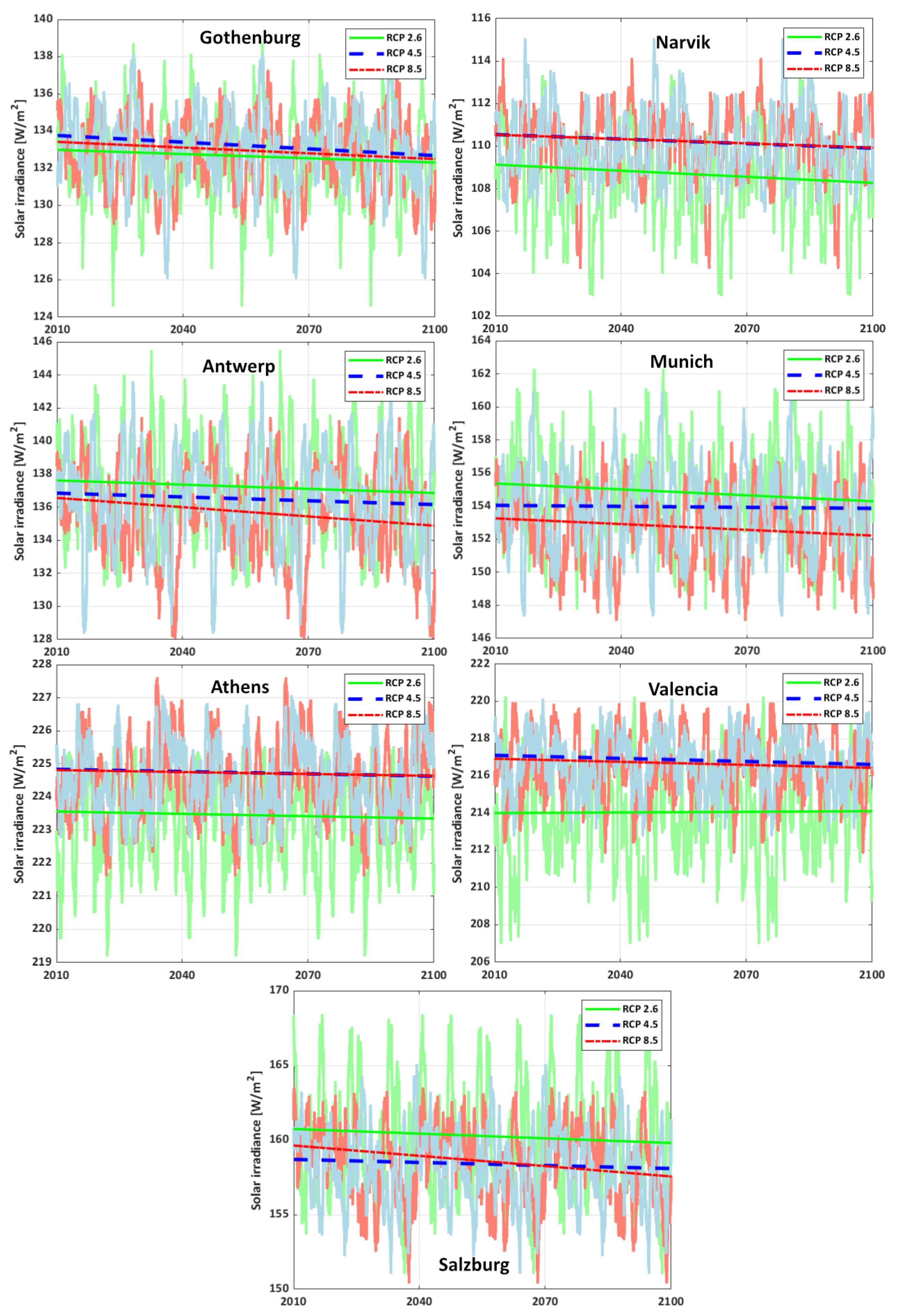
3.1. Long-Term Trends of Solar and Wind Energy Potential

The regression analysis in Figure 1 shows the long-term solar irradiance trends and variations over time for RCP 2.6, RCP 4.5, and RCP 8.5. Each regression line combines all five GCMs. According to the results, for each combination of GCM, all RCPs show a decreasing trend for solar irradiance throughout 2010–2099 (regression equations in

Table 1. Regression analysis for solar irradiance and wind speed of 7 European cities.

City	Solar RCP 2.6	Solar RCP 4.5	Solar RCP 8.5	Wind RCP 2.6	Wind RCP 4.5	Wind RCP 8.5
Gothenburg	y = −8.9 × 10−7x + 132	y = −1.4 × 10−6x + 133	y = −1.2 × 10−6x + 133	y = −1.9 × 10−7x + 4.7	y = −1.1 × 10−7x + 4.6	y = −2.4 × 10−8x + 4.6
Narvik	y = −1.1 × 10−6x + 109	y = −8.3 × 10−7x + 110	y = −7.9 × 10−7x + 110	y = −2.1 × 10−7x + 5.1	y = −1.4 × 10−7x + 4.9	y = −3.1 × 10−7x + 4.9
Antwerp	y = −9.9 × 10−7x + 137	y = −8.9 × 10−7x + 136	y = −2.1 × 10−6x + 136	y = −6.5 × 10−8x + 4.2	y = −7.2 × 10−8x + 4.2	y = −3.2 × 10−8x + 4.2
Munich	y = −1.4 × 10−6x + 155	y = −2.3 × 10−7x + 154	y = −1.3 × 10−6x + 153	y = −5.6 × 10−8x + (4.2	y = −7.1 × 10−8x + 4.3	y = 7.3 × 10−10x + 4.3
Athens	y = −2.7 × 10−7x + 223	y = −2.6 × 10−7x + 224	y = −2.2 × 10−7x + 224	y = −1.2 × 10−7x + 4.2	y = 8.1 × 10−9x + 4.2	y = 2.5 × 10−8x + 4.2
Valencia	y = −1.3 × 10−7x + 213	y = −6.4 × 10−7x + 217	y = −6.4 × 10−7x + 216	y = 1.17 × 10−8x + 3.4	y = −2.1 × 10−7x + 3.6	y = −2.9 × 10−7x + 3.6
Salzburg	y = −1.2 × 10−6x + 160	y = −7.9 × 10−7x + 158	y = −2.6 × 10−6x + 159	y = −7.6 × 10−8x + (3.3	y = −1.2 × 10−7x + 3.4	y = −1.2 × 10−7x + 3.4
Coefficient of determination (R2)	Solar RCP 2.6	Solar RCP 4.5	Solar RCP 8.5	Wind RCP 2.6	Wind RCP 4.5	Wind RCP 8.5
Gothenburg	0.04	0.01	0.09	0.09	0.05	0.02
Narvik	0.01	0.04	0.04	0.09	0.07	0.3
Antwerp	0.04	0.04	0.02	0.01	0.02	0.04
Munich	0.01	0.03	0.01	0.02	0.03	0.02
Athens	0.06	0.07	0.04	0.09	0.08	0.07
Valencia	0.08	0.03	0.03	0.24	0.21	0.36
Salzburg	0.04	0.03	0.04	0.03	0.13	0.1

). Among the seven cities, Gothenburg has the fastest decreasing trend followed by Antwerp and Narvik. Athens has the highest solar irradiance among all the cities, followed by Valencia. These two cities have the lowest decreasing rate of solar irradiance due to climate change.

The regression analysis for wind speed was performed, along with the determination coefficient (R²) (see Figure 2 and Table 1). It can be found that Athens has a significant upward trend in RCP 4.5 and RCP 8.5, while Valencia and Munich only have a slightly increasing trend in RCP 2.6 and RCP 8.5, respectively. Except for the cases mentioned above, the other ones all show an overall decreasing trend. Among them, Valencia has the most apparent decreasing trend in RCP 8.5, followed by Narvik and Salzburg. Compared to solar irradiance, the scattered points are more dispersed around the regression line, and the decreasing or increasing trend is more visible.

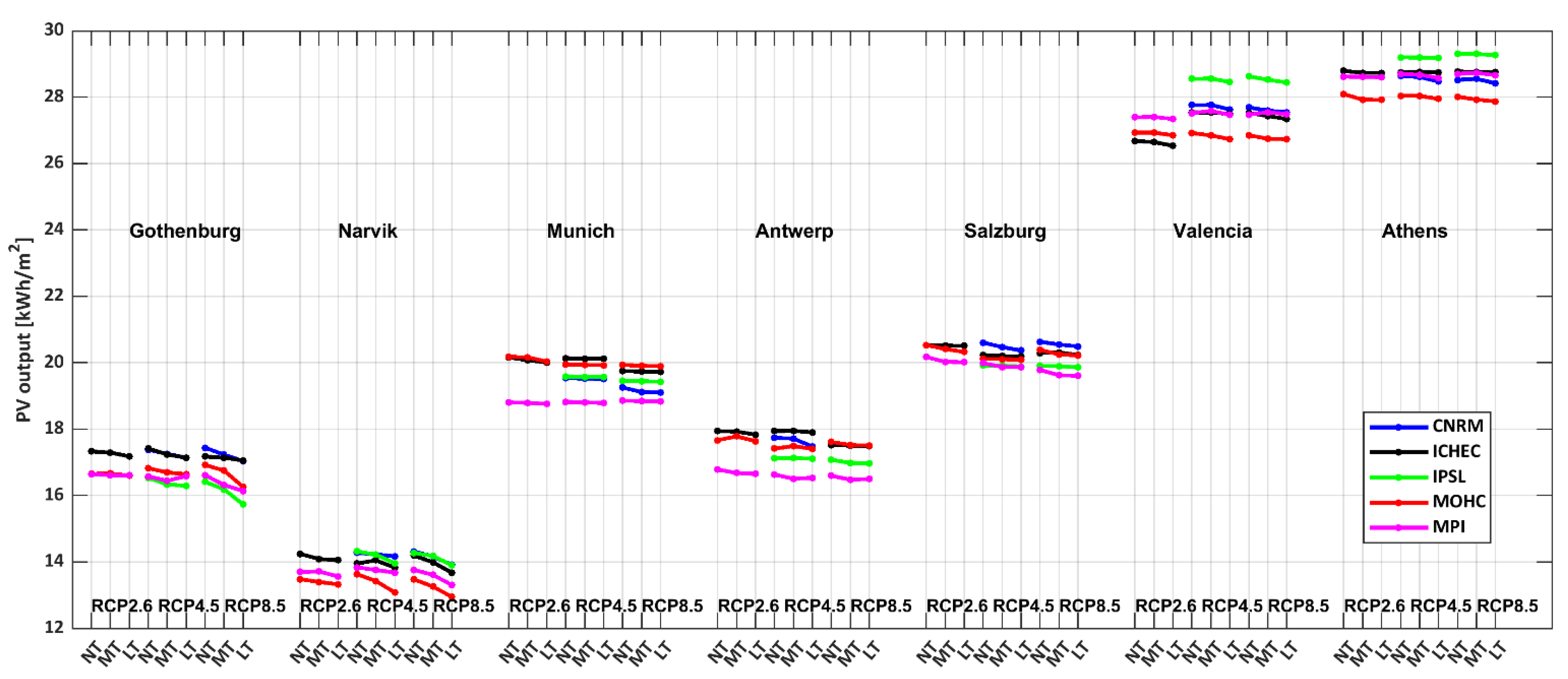
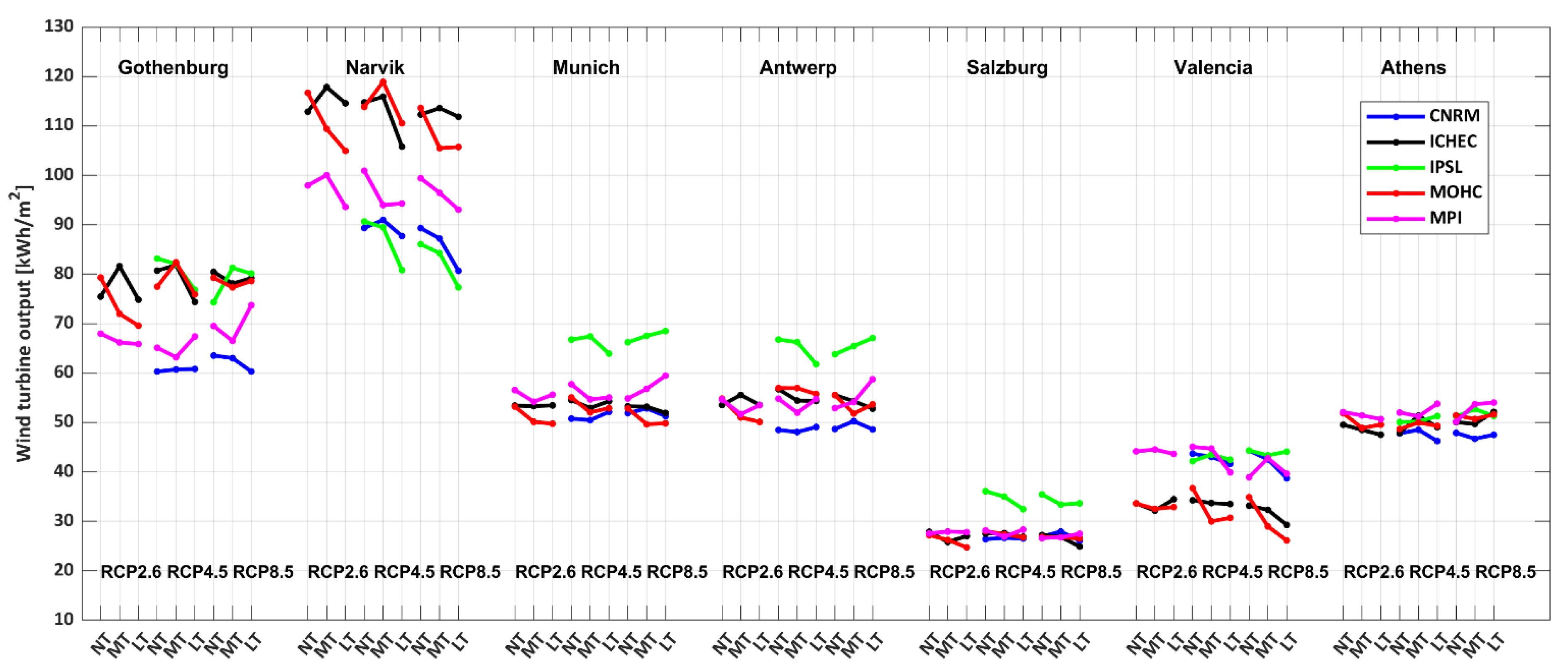
3.2. Long-Term Variations Due to Climate Change and Uncertainties

The impact of climate change on average PV output is shown in Figure 3. For all RCPs and GCMs, the output of PV has a downward trend over time, but the relative differences are very small, which are discussed in the following section in

Table 2. Relative difference of NT–MT and MT–LT of PV output for each climate scenario.

GCM	Gothenburg	Narvik	Munich	Antwerp	Salzburg	Valencia	Athens
CNRM45 NT–MT	−0.05%	−0.09%	−0.10%	−0.86%	−0.67%	−0.48%	−0.10%
CNRM45 MT–LT	−0.50%	−0.03%	−0.57%	−0.53%	−0.35%	−1.46%	−0.73%
CNRM85 NT–MT	−0.74%	−0.55%	−0.42%	−1.69%	−2.05%	−0.95%	−0.03%
CNRM85 MT–LT	−1.12%	−1.05%	−1.65%	−0.15%	−1.97%	−0.49%	−0.77%
ICHEC26 NT–MT	−0.71%	−0.45%	−0.49%	−0.55%	−1.87%	−0.44%	−0.20%
ICHEC26 MT–LT	−0.20%	−0.40%	−1.32%	−1.49%	−0.23%	−0.04%	−0.25%
ICHEC45 NT–MT	−1.10%	−1.13%	−0.74%	−0.51%	−1.61%	−1.22%	−0.23%
ICHEC45 MT–LT	−1.52%	−1.91%	−1.47%	−1.66%	−0.70%	−0.93%	−0.14%
ICHEC85 NT–MT	−1.23%	−1.30%	−0.88%	−1.20%	−0.97%	−0.17%	−0.12%
ICHEC85 MT–LT	−0.07%	−1.29%	−1.80%	−1.47%	−1.78%	−0.31%	−0.17%
IPSL45 NT–MT	−0.76%	−0.85%	−1.31%	−0.47%	−0.62%	−0.02%	−0.28%
IPSL45 MT–LT	−0.40%	−1.56%	−0.88%	−0.28%	−0.59%	−1.00%	−0.45%
IPSL85 NT–MT	−1.72%	−0.47%	−2.13%	−0.08%	−1.95%	−0.23%	−0.41%
IPSL85 MT–LT	−1.19%	−1.17%	−2.17%	−0.40%	−0.85%	−0.26%	−0.93%
MOHC26 NT–MT	−0.01%	−1.09%	−1.69%	−1.70%	−0.90%	−0.29%	−0.18%
MOHC26 MT–LT	−1.07%	−1.31%	−1.50%	−0.40%	−0.31%	−0.02%	−0.03%
MOHC45 NT–MT	−0.08%	−0.95%	−1.91%	−1.83%	−1.68%	−0.24%	−0.08%
MOHC45 MT–LT	−0.34%	−0.92%	−0.92%	−1.20%	−1.66%	−0.45%	−0.47%
MOHC85 NT–MT	−1.82%	−1.03%	−0.48%	−0.59%	−0.08%	−0.37%	−0.38%
MOHC85 MT–LT	−0.05%	−1.15%	−1.81%	−2.04%	−2.00%	−0.26%	−0.76%
MPI26 NT–MT	−0.49%	−0.44%	−1.97%	−2.29%	−1.36%	−0.25%	−0.29%
MPI26 MT–LT	−2.43%	−0.46%	−1.33%	−2.21%	−1.16%	−0.57%	−0.01%
MPI45 NT–MT	−0.57%	−1.24%	−0.86%	−0.22%	−0.92%	−0.14%	−0.19%
MPI45 MT–LT	−0.47%	−1.36%	−1.41%	−2.63%	−1.01%	−0.21%	−0.11%
MPI85 NT–MT	−1.85%	−1.55%	−1.48%	−0.59%	−0.43%	−0.10%	−0.16%
MPI85 MT–LT	−0.28%	−1.83%	−1.73%	−1.01%	−1.54%	−0.43%	−0.51%

and

Table 3. Relative difference of NT–MT and MT–LT of winter wind turbine output for each climate scenario.

GCM	Gothenburg	Narvik	Munich	Antwerp	Salzburg	Valencia	Athens
CNRM45 NT–MT	−2.6%	−3.0%	4.4%	1.3%	−3.6%	10.6%	2.7%
CNRM45 MT–LT	−6.6%	−0.5%	−5.8%	−8.4%	−1.6%	7.1%	1.7%
CNRM85 NT–MT	2.3%	3.8%	−3.3%	−3.6%	−3.3%	−4.1%	1.6%
CNRM85 MT–LT	1.0%	11.3%	1.6%	−0.2%	4.7%	15.7%	−4.8%
ICHEC26 NT–MT	−12.1%	−6.3%	−1.0%	−5.5%	7.9%	−0.3%	5.4%
ICHEC26 MT–LT	11.1%	6.6%	−3.7%	4.0%	−2.5%	−6.4%	−4.6%
ICHEC45 NT–MT	4.8%	5.6%	4.5%	7.2%	−3.2%	−13.4%	−9.7%
ICHEC45 MT–LT	11.0%	12.8%	−3.7%	−5.4%	4.6%	9.5%	12.4%
ICHEC85 NT–MT	0.1%	−4.1%	5.6%	2.8%	−4.1%	12.1%	2.1%
ICHEC85 MT–LT	−0.2%	5.8%	−2.0%	2.8%	13.5%	−7.3%	−0.5%
IPSL45 NT–MT	9.6%	2.8%	−2.4%	4.0%	8.0%	−10.7%	2.8%
IPSL45 MT–LT	4.3%	8.0%	10.5%	9.2%	8.4%	6.0%	2.8%
IPSL85 NT–MT	−13.3%	4.6%	−6.5%	−5.5%	8.9%	1.1%	7.8%
IPSL85 MT–LT	−4.8%	3.7%	0.0%	−3.4%	−1.6%	−7.8%	1.0%
MOHC26 NT–MT	6.6%	13.2%	9.5%	8.6%	8.6%	7.1%	−4.6%
MOHC26 MT–LT	7.2%	5.0%	0.1%	4.9%	6.4%	−13.1%	2.9%
MOHC45 NT–MT	−15.0%	−7.4%	1.3%	−7.4%	−2.5%	22.3%	0.6%
MOHC45 MT–LT	19.8%	11.3%	4.1%	11.3%	6.0%	−12.4%	1.2%
MOHC85 NT–MT	8.1%	20.4%	11.2%	10.8%	1.4%	15.4%	−5.2%
MOHC85 MT–LT	−1.1%	−2.9%	−5.5%	−7.7%	−4.1%	15.6%	−2.0%
MPI26 NT–MT	4.6%	−3.7%	7.1%	12.1%	6.0%	−12.0%	10.3%
MPI26 MT–LT	−6.8%	4.9%	−4.1%	−9.7%	0.0%	6.3%	−4.5%
MPI45 NT–MT	3.3%	18.9%	9.8%	9.0%	3.3%	−1.4%	1.4%
MPI45 MT–LT	−9.9%	−2.6%	−11.6%	−14.9%	−8.1%	9.3%	−2.8%
MPI85 NT–MT	12.1%	2.3%	−9.8%	−6.7%	−4.5%	−22.4%	−10.5%
MPI85 MT–LT	−12.5%	0.8%	−6.4%	−10.9%	−0.2%	10.1%	8.3%

. ICHEC-RCP 2.6 predicts a relatively higher PV output than the other GCMs in the seven cities in Figure 4. For example, in Munich, ICHEC projects a 13.2% higher PV production than MPI. For RCP 4.5 and RCP 8.5, IPSL in Valencia, Athens, and Norway predicts larger PV outputs. For example, IPSL in Athens is 2.7% and 3.6% higher than MPI-RCP 4.5 and -RCP 8.5, respectively. Different RCPs for the same GCM induce small changes in the PV output. For example, in Munich, RCP 8.5 for MOHC is 0.03% lower than RCP 2.6. Regarding the projection of wind energy, all the GCMs showed an irregular change between NT, MT, and LT (see Figure 4). For RCP 2.6, MOHC and MPI have a decreasing trend in seven cities, while ICHEC shows a different trend. For example, in Gothenburg and Narvik, ICHEC shows an increasing trend in the MT. For both PV and wind turbine outputs, the numbers do not change considerably between the 30-year periods.

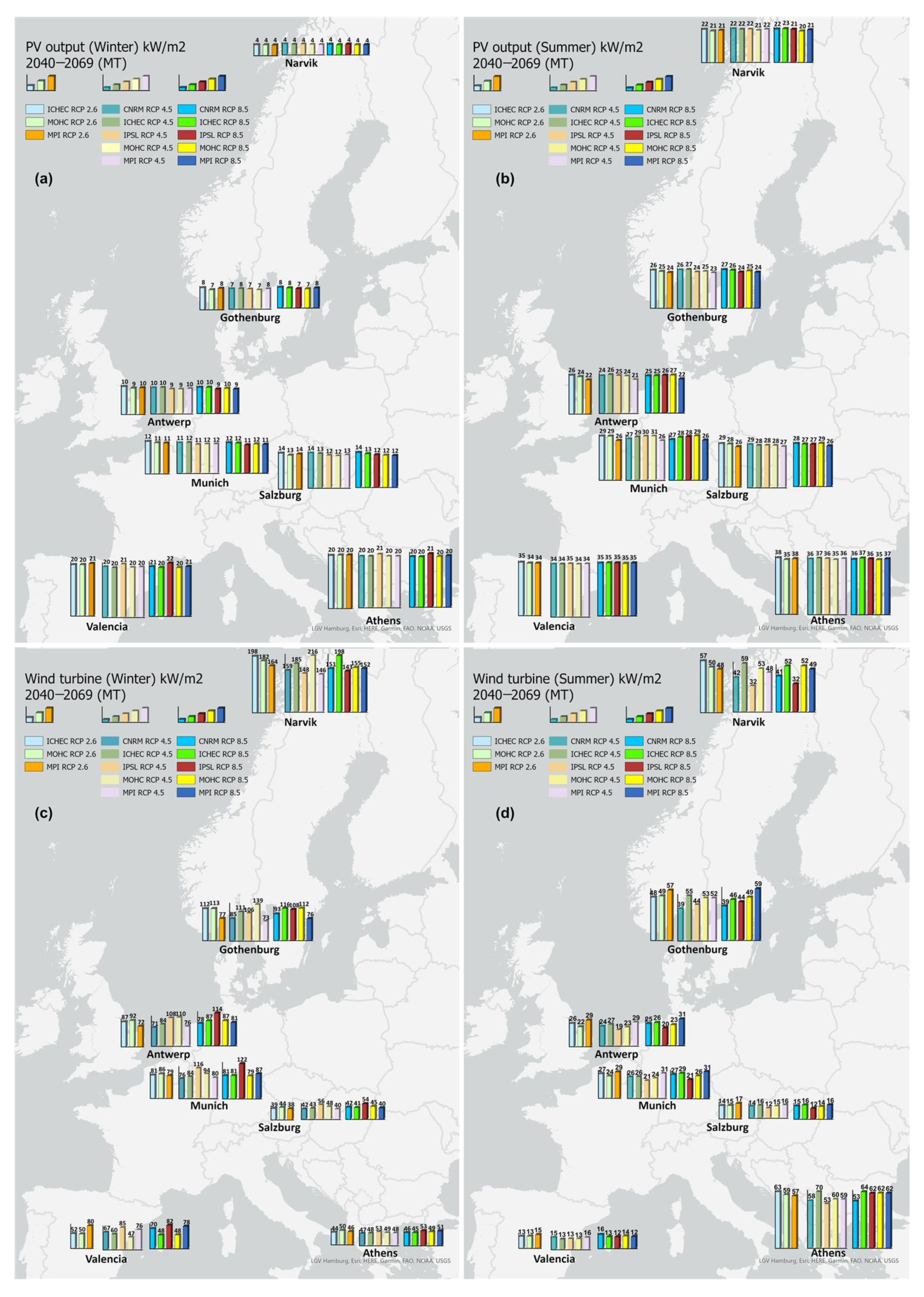
3.3. Seasonal PV and Wind Energy Potential and Their Variations

This section assesses seasonal photovoltaic and wind energy potential, considering summer (June to August) and winter (December to March). Figure 5a,b show PV output results in the MT considering 13 climate scenarios, clearly showing that the summer PV output is higher than that in winter. In summer, Athens has the highest PV output (35 kWh/m²–38 kWh/m²), followed by Valencia (34 kWh/m²–35 kWh/m²). The PV production in Antwerp, Munich Salzburg, and Narvik vary from 22 kWh/m² to 29 kWh/m². Winter PV outputs show a similar pattern with smaller values. Seasonal wind turbine output behaves contrary to PV production (see Figure 5c,d). For example, in winter, Narvik produces almost three times more energy than in summer (146 kWh/m²–198 kWh/m² in winter and 32 kWh/m²–59 kWh/m² in summer). Gothenburg, Antwerp, Munich, Salzburg, and Valencia also show the same trend, having about 2.4 times higher wind energy in winter compared to summer. The seasonal variations and complementarity characteristics of wind and solar energy are interesting. For example, when Narvik has limited PV output in winter (6 kWh/m²–7 kWh/m²), the wind energy is about 10 times that of the PV output, which has the best temporal complementarity.

The seasonal relative differences of NT–MT and MT–LT for PV productions are shown in Table 2 (summer) and for wind turbines in Table 3 (winter). The differences due to time period (climate change), GCM, and RCP (climate uncertainties) are visible for both PV and wind potential. For PV output, an evident decline was found across all time periods, but the relative differences are minimal. For example, the relative difference between Gothenburg NT–MT and MT–LT is between −0.1% and 0.86%. In general, the difference due to the time period changes is much smaller than that induced by selecting climate scenarios (climate uncertainty). For example, the maximum relative differences for NT–MT and MT–LT range from −0.01% to −2.17% for the entire period. However, the differences between selection climate scenarios are up to 12% (e.g., for Munich between MOHC-RCP 8.5 and MPI-RCP 8.5 in the MT in Figure 5).

For wind potential, the relative differences are much higher than those for PV. Due to the climate uncertainties, there is no general trend for wind energy potential suggesting its increase or decrease over time. For example, in winter (Figure 5d), the relative difference between ICHEC-RCP 4.5 and IPSL-RCP 4.5 in Narvik is 45%, while the maximum relative difference for the entire period is only 22% (Table 2). Differences between RCPs for the same GCM also have a larger relative difference in wind turbine output.

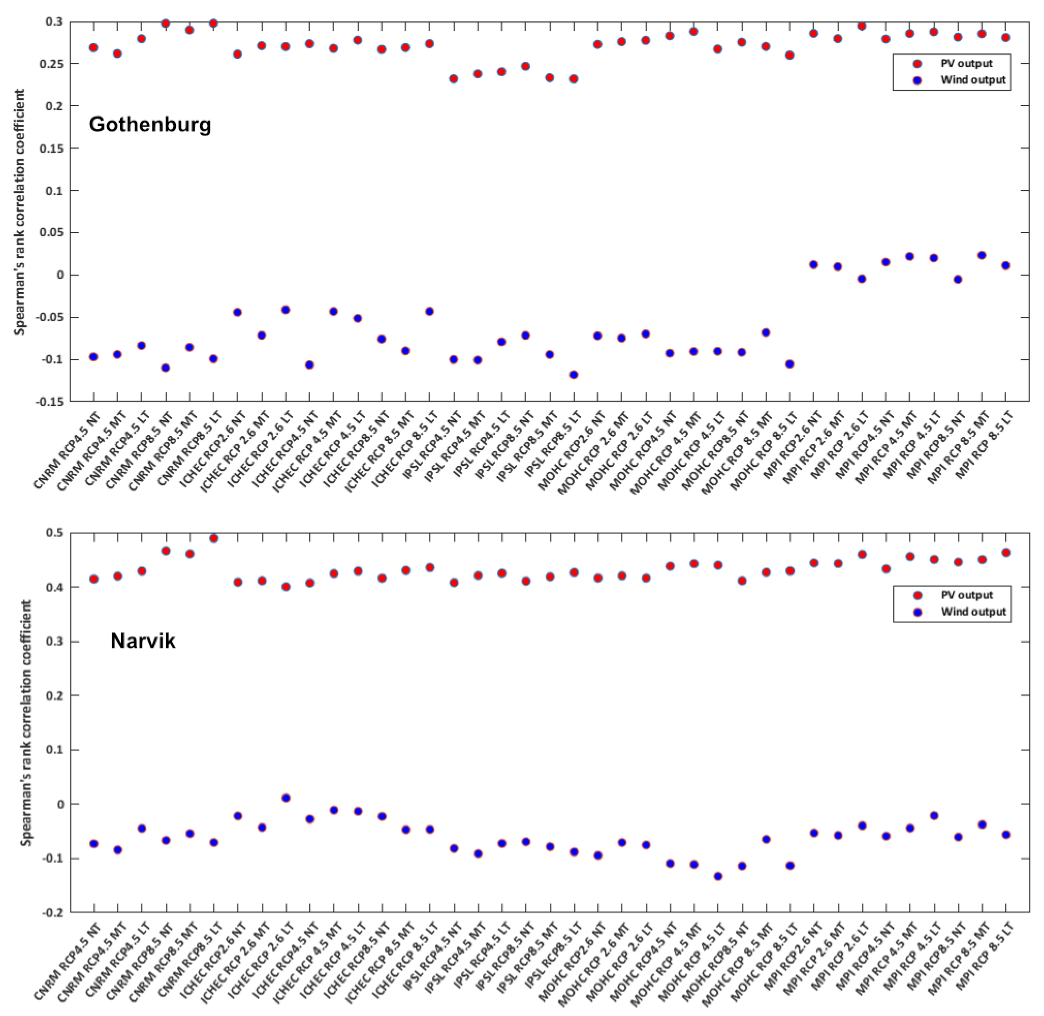
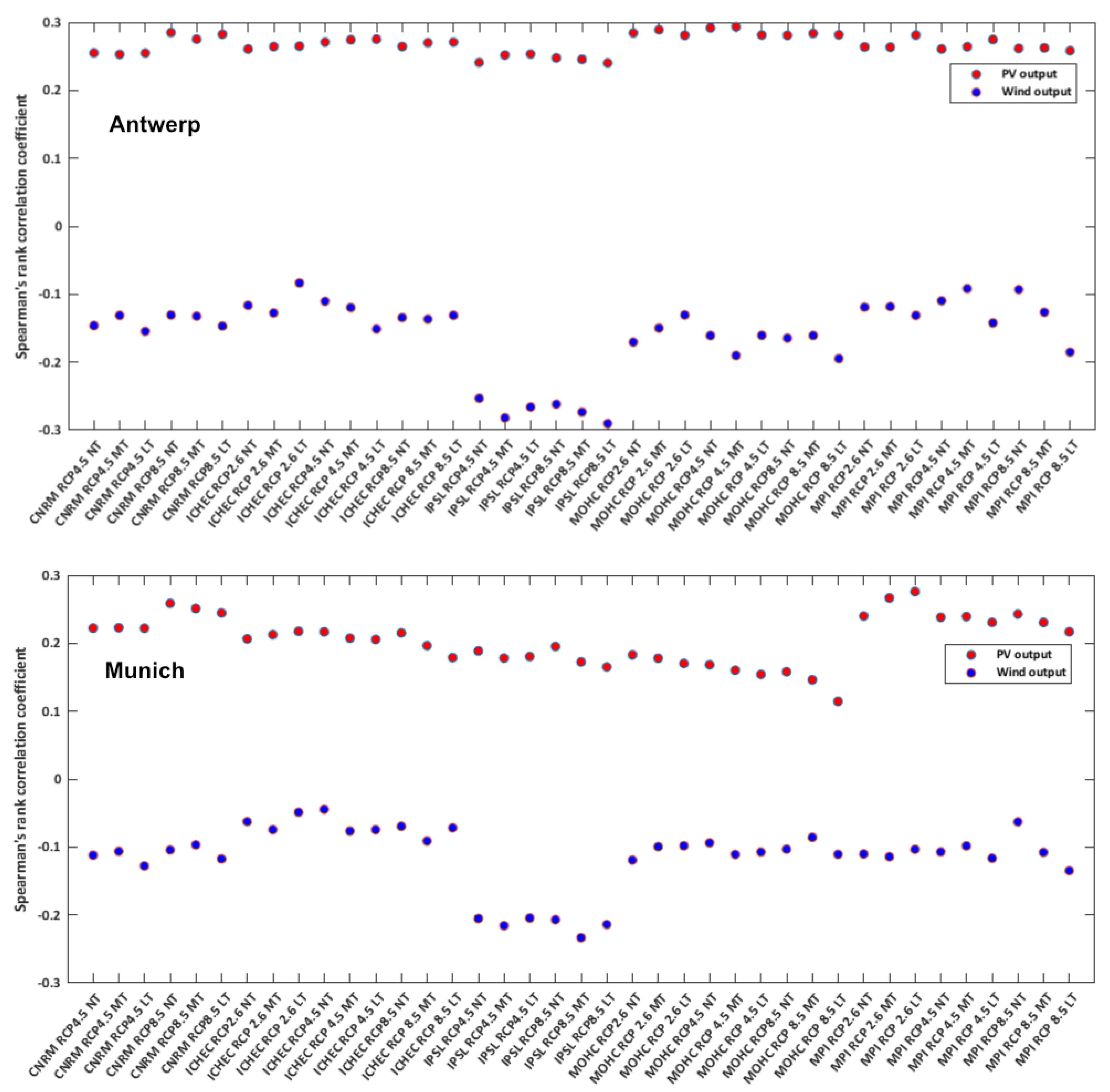
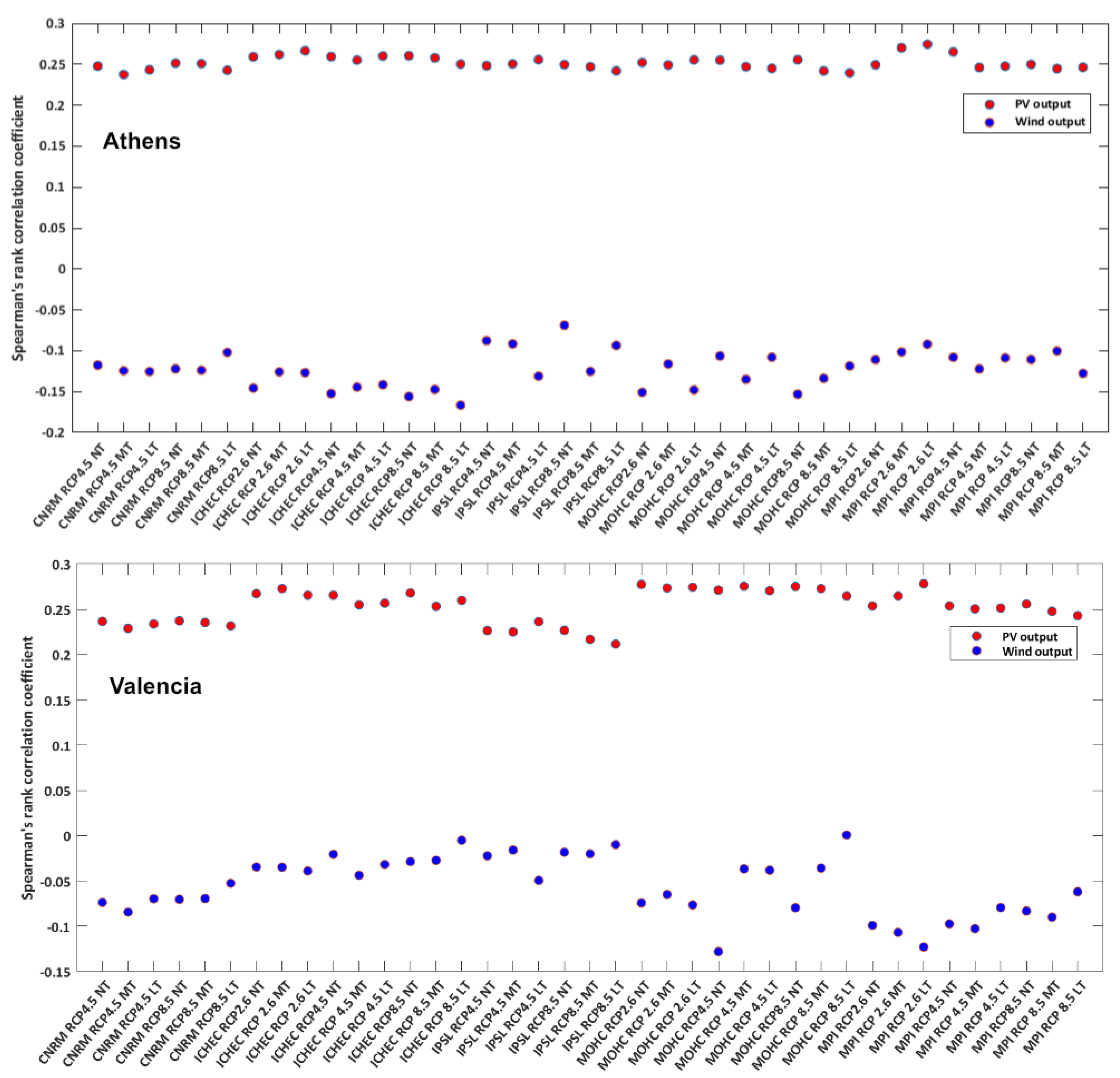
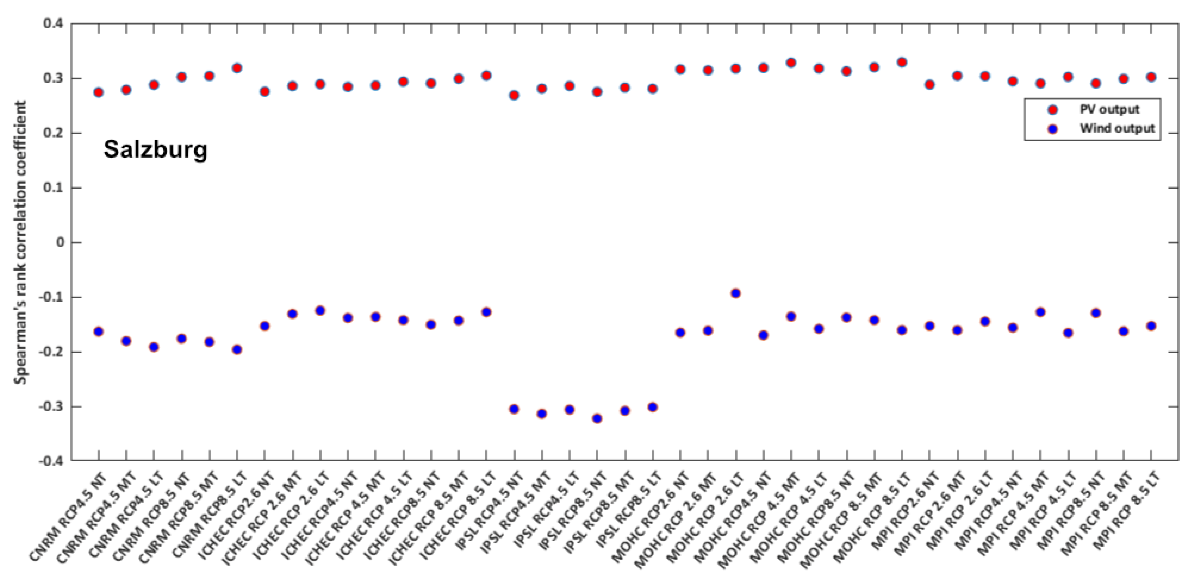
3.4. Spearman’s Correlation Analysis

To further explore the uncertainties in the projected PV and wind potential, Spearman’s rank correlation was calculated between the hourly temperature and hourly PV or wind turbine energy generation potential. As explained in Section 2, Spearman’s rank correlation is calculated to check the agreement on the ranking results between two groups, in which group 1 is the hourly temperature from the different climate scenarios and group 2 is the hourly PV output or wind turbine output. In general, the result indicates that outdoor temperature is positively correlated to PV output and negatively correlated to wind output. From Figure 6, Figure 7, Figure 8 and Figure 9, the correlation between outdoor temperature and relevant output varies differently due to climate uncertainty. For example, the correlation between outdoor temperature and wind output in Antwerp, Munich, and Salzburg for IPSL showed a strong negative correlation in all periods and RCPs, with a correlation coefficient between −0.27 and 0.33. In contrast, the correlation in other climate scenarios did not reflect such a strong negative correlation (around 0.2). A similar result also appears in Gothenburg; the temperature and wind output show a near-zero correlation in all scenarios for MPI, while the other scenarios project negative correlations. For the correlation coefficient between outdoor temperature and PV output, which remains in the range of 0.23–0.4 for all the cities, due to the uncertainty, some scenarios project a weak correlation; for example, IPSL in Gothenburg projects less correlation (0.23–0.27) and CNRM RCP 8.5 and MPI RCP 2.6 in Munich project a higher correlation compared with other scenarios.

4. Conclusions

This work investigated the impacts of future climate uncertainties on projecting the renewable energy generation potential (solar PV and wind). This study showed how climate change can affect renewable energy generation in seven European countries distributed over five different European climate zones. In this regard, the potential changes in climate variables related to future photovoltaic (solar irradiance) and wind power generation (wind speed), based on CMIP5 climate change projections under the framework of the fifth IPCC assessment report, were quantified. The GCM data have been dynamically downscaled by RCA4, with hourly temporal resolution and 12.5km² spatial resolution, allowing us to access both long-term and short-term variations in the climate. The solar radiation and wind speed projections over the period of 2010–2099 were used considering five GCMs forced by RCP 2.6, RCP 4.6, and RCP 8.5.

The results showed that the overall future PV and wind potential do not change considerably by climate change. In all climate scenarios, an overall decrease in PV potential is found, but the relative change is about 0.01–2.71%. For wind turbine potential, the RCP 8.5 of Gothenburg, Antwerp, Munich, and Athens increased slightly by 0.6–2.3%. The temporal complementarity that exists between solar and wind resources in the seasonal scale does not change considerably by climate change. Spearman’s rank correlation indicates a positive correlation between outdoor temperature with PV output and a negative correlation with wind output. For the seasonal variations, the uncertainties associated with different climate scenarios considerably affect the renewable energy output. Based on the assessment, differences induced by climate evolution (i.e., when comparing different time periods) are smaller—varying around 0.01–2.17% for PV output and around 22% for wind output—than those induced by climate uncertainties (i.e., when comparing different climate scenarios), reaching up to 23% for PV output and 45% for wind turbine output. The results of Spearman’s correlation analysis revealed strong correlations between outdoor temperature and PV output for some scenarios (e.g., a strong positive correlation of 0.4–0.5 in Narvik) and wind turbine output generation (e.g., a strong negative correlation from −0.27 to −0.33 for IPSL in Antwerp, Munich, and Salzburg).

The results indicated the importance of considering multiple climate scenarios and accounting for climate uncertainties when planning for future energy solutions. This can be very important when planning for the climate change adaptation of future cities. The proposed methodology to account for climate uncertainties and short-/long-term variations can be applied to other regions. The developed projection database has the potential to be adopted as a reliable source to support the expansion of energy systems that rely on renewable energy or countries that plan to expand their renewable energy networks.

References

1. Sadik-Zada, E.R.; Gatto, A. Energy Security Pathways in South East Europe: Diversification of the Natural Gas Supplies, Energy Transition, and Energy Futures. In From Economic to Energy Transition: Three Decades of Transitions in Central and Eastern Europe; Mišík, M., Oravcová, V., Eds.; Energy, Climate and the Environment; Springer International Publishing: Cham, Switzerland, 2021; pp. 491–514. ISBN 978-3-030-55085-1. [Google Scholar]
2. Edenhofer, O. (Ed.) Climate Change 2014: Mitigation of Climate Change: Working Group III Contribution to the Fifth Assessment Report of the Intergovernmental Panel on Climate Change; Intergovernmental Panel on Climate Change; Cambridge University Press: New York, NY, USA, 2014; ISBN 978-1-107-05821-7. [Google Scholar]
3. Renewable Energy Statistics—Statistics Explained. Available online: https://ec.europa.eu/eurostat/statistics-explained/index.php/Renewable_energy_statistics#Share_of_renewable_energy_almost_doubled_between_2004_and_2018 (accessed on 1 February 2021).
4. Solar PV—Renewables 2020—Analysis—IEA. Available online: https://www.iea.org/reports/renewables-2020/solar-pv (accessed on 21 February 2021).
5. UN. Paris Agreement; 6 United Nations Framework Convention on Climate Change (UNFCCC): Paris, France, 2016; Volume 55. [Google Scholar]
6. EU Power Sector in 2020. Available online: https://static.agora-energiewende.de/fileadmin/Projekte/2021/2020_01_EU-Annual-Review_2020/A-EW_202_Report_European-Power-Sector-2020.pdf (accessed on 27 December 2021).
7. Anonymous. 2030 Climate & Energy Framework. Available online: https://ec.europa.eu/clima/policies/strategies/2030_en (accessed on 25 February 2021).
8. Brodny, J.; Tutak, M.; Bindzár, P. Assessing the Level of Renewable Energy Development in the European Union Member States. A 10-Year Perspective. Energies 2021, 14, 3765. [Google Scholar] [CrossRef]
9. Perera, A.T.D.; Javanroodi, K.; Wang, Y.; Hong, T. Urban Cells: Extending the Energy Hub Concept to Facilitate Sector and Spatial Coupling. Adv. Appl. Energy 2021, 3, 100046. [Google Scholar] [CrossRef]
10. Sadik-Zada, E.R. Political Economy of Green Hydrogen Rollout: A Global Perspective. Sustainability 2021, 13, 13464. [Google Scholar] [CrossRef]
11. Actions Being Taken by the EU. Available online: https://ec.europa.eu/info/strategy/priorities-2019-2024/european-green-deal/actions-being-taken-eu_en (accessed on 1 February 2021).
12. Alberini, A.; Prettico, G.; Shen, C.; Torriti, J. Hot Weather and Residential Hourly Electricity Demand in Italy. Energy 2019, 177, 44–56. [Google Scholar] [CrossRef]
13. Silva, S.; Soares, I.; Pinho, C. Climate Change Impacts on Electricity Demand: The Case of a Southern European Country. Util. Policy 2020, 67, 101115. [Google Scholar] [CrossRef]
14. Bloomfield, H.C.; Brayshaw, D.J.; Troccoli, A.; Goodess, C.M.; De Felice, M.; Dubus, L.; Bett, P.E.; Saint-Drenan, Y.-M. Quantifying the Sensitivity of European Power Systems to Energy Scenarios and Climate Change Projections. Renew. Energy 2021, 164, 1062–1075. [Google Scholar] [CrossRef]
15. Pachauri, R.K.; Meyer, L.; Hallegatte France, S.; Bank, W.; Hegerl, G.; Brinkman, S.; van Kesteren, L.; Leprince-Ringuet, N.; van Boxmeer, F. IPCC Climate Change 2014: Synthesis Report; Gian-Kasper Plattner: Geneva, Switzerland, 2014; ISBN 978-92-9169-143-2. [Google Scholar]
16. Chen, L. Uncertainties in Solar Radiation Assessment in the United States Using Climate Models. Clim. Dyn. 2021, 56, 665–678. [Google Scholar] [CrossRef]
17. Fant, C.; Adam Schlosser, C.; Strzepek, K. The Impact of Climate Change on Wind and Solar Resources in Southern Africa. Appl. Energy 2016, 161, 556–564. [Google Scholar] [CrossRef] [Green Version]
18. Huang, G.; Li, Z.; Li, X.; Liang, S.; Yang, K.; Wang, D.; Zhang, Y. Estimating Surface Solar Irradiance from Satellites: Past, Present, and Future Perspectives. Remote Sens. Environ. 2019, 233, 111371. [Google Scholar] [CrossRef]
19. Randall, D.A.; Wood, R.A.; Bony, S.; Colman, R.; Fichefet, T.; Fyfe, J.; Kattsov, V.; Pitman, A.; Shukla, J.; Srinivasan, J.; et al. Climate Models and Their Evaluation; Cambridge University Press: Cambridge, UK, 2007; p. 74. [Google Scholar]
20. Viviescas, C.; Lima, L.; Diuana, F.A.; Vasquez, E.; Ludovique, C.; Silva, G.N.; Huback, V.; Magalar, L.; Szklo, A.; Lucena, A.F.P.; et al. Contribution of Variable Renewable Energy to Increase Energy Security in Latin America: Complementarity and Climate Change Impacts on Wind and Solar Resources. Renew. Sustain. Energy Rev. 2019, 113, 109232. [Google Scholar] [CrossRef]
21. Oka, K.; Mizutani, W.; Ashina, S. Climate Change Impacts on Potential Solar Energy Production: A Study Case in Fukushima, Japan. Renew. Energy 2020, 153, 249–260. [Google Scholar] [CrossRef]
22. Pryor, S.C.; Schoof, J.T.; Barthelmie, R.J. Winds of Change? Projections of near-Surface Winds under Climate Change Scenarios. Geophys. Res. Lett. 2006, 33, L11702. [Google Scholar] [CrossRef] [Green Version]
23. Yang, Y.; Javanroodi, K.; Nik, V.M. Climate Change and Energy Performance of European Residential Building Stocks—A Comprehensive Impact Assessment Using Climate Big Data from the Coordinated Regional Climate Downscaling Experiment. Appl. Energy 2021, 298, 117246. [Google Scholar] [CrossRef]
24. Perera, A.T.D.; Nik, V.M.; Chen, D.; Scartezzini, J.L.; Hong, T. Quantifying the Impacts of Climate Change and Extreme Climate Events on Energy Systems. Nat. Energy 2020, 5, 150–159. [Google Scholar] [CrossRef] [Green Version]
25. Yang, Y.; Javanroodi, K.; Nik, V.M. Impact Assessment of Climate Change on the Energy Performance of the Building Stocks in Four European Cities. E3S Web Conf. 2020, 172, 02008. [Google Scholar] [CrossRef]
26. Perera, A.T.D.; Javanroodi, K.; Nik, V.M. Climate Resilient Interconnected Infrastructure: Co-Optimization of Energy Systems and Urban Morphology. Appl. Energy 2021, 285, 116430. [Google Scholar] [CrossRef]
27. Weber, J.; Gotzens, F.; Witthaut, D. Impact of Strong Climate Change on the Statistics of Wind Power Generation in Europe. Energy Procedia 2018, 153, 22–28. [Google Scholar] [CrossRef]
28. Moemken, J.; Reyers, M.; Feldmann, H.; Pinto, J.G. Future Changes of Wind Speed and Wind Energy Potentials in EURO-CORDEX Ensemble Simulations. J. Geophys. Res. Atmos. 2018, 123, 6373–6389. [Google Scholar] [CrossRef]
29. Reyers, M.; Moemken, J.; Pinto, J.G. Future Changes of Wind Energy Potentials over Europe in a Large CMIP5 Multi-Model Ensemble. Int. J. Climatol. 2016, 36, 783–796. [Google Scholar] [CrossRef]
30. Tobin, I.; Jerez, S.; Vautard, R.; Thais, F.; van Meijgaard, E.; Prein, A.; Déqué, M.; Kotlarski, S.; Maule, C.F.; Nikulin, G.; et al. Climate Change Impacts on the Power Generation Potential of a European Mid-Century Wind Farms Scenario. Environ. Res. Lett. 2016, 11, 034013. [Google Scholar] [CrossRef]
31. Jerez, S.; Tobin, I.; Vautard, R.; Montávez, J.P.; López-Romero, J.M.; Thais, F.; Bartok, B.; Christensen, O.B.; Colette, A.; Déqué, M.; et al. The Impact of Climate Change on Photovoltaic Power Generation in Europe. Nat. Commun. 2015, 6, 10014. [Google Scholar] [CrossRef] [Green Version]
32. Wild, M.; Folini, D.; Henschel, F.; Fischer, N.; Müller, B. Projections of Long-Term Changes in Solar Radiation Based on CMIP5 Climate Models and Their Influence on Energy Yields of Photovoltaic Systems. Sol. Energy 2015, 116, 12–24. [Google Scholar] [CrossRef] [Green Version]
33. Panagea, I.S.; Tsanis, I.K.; Koutroulis, A.G.; Grillakis, M.G. Climate Change Impact on Photovoltaic Energy Output: The Case of Greece. Available online: https://www.hindawi.com/journals/amete/2014/264506/ (accessed on 1 March 2021).
34. Müller, J.; Folini, D.; Wild, M.; Pfenninger, S. CMIP-5 Models Project Photovoltaics Are a No-Regrets Investment in Europe Irrespective of Climate Change. Energy 2019, 171, 135–148. [Google Scholar] [CrossRef]
35. Nik, V.M. Making Energy Simulation Easier for Future Climate—Synthesizing Typical and Extreme Weather Data Sets out of Regional Climate Models (RCMs). Appl. Energy 2016, 177, 204–226. [Google Scholar] [CrossRef]
36. Riahi, K.; van Vuuren, D.P.; Kriegler, E.; Edmonds, J.; O’Neill, B.C.; Fujimori, S.; Bauer, N.; Calvin, K.; Dellink, R.; Fricko, O.; et al. The Shared Socioeconomic Pathways and Their Energy, Land Use, and Greenhouse Gas Emissions Implications: An Overview. Glob. Environ. Chang. 2017, 42, 153–168. [Google Scholar] [CrossRef] [Green Version]
37. van Vuuren, D.P.; Riahi, K.; Moss, R.; Edmonds, J.; Thomson, A.; Nakicenovic, N.; Kram, T.; Berkhout, F.; Swart, R.; Janetos, A.; et al. A Proposal for a New Scenario Framework to Support Research and Assessment in Different Climate Research Communities. Glob. Environ. Chang. 2012, 22, 21–35. [Google Scholar] [CrossRef] [Green Version]
38. Vad Är RCP? | SMHI. Available online: https://www.smhi.se/klimat/framtidens-klimat/vagledning-klimatscenarier/vad-ar-rcp-1.80271 (accessed on 30 November 2020).
39. Navarro-Racines, C.; Tarapues, J.; Thornton, P.; Jarvis, A.; Ramirez-Villegas, J. High-Resolution and Bias-Corrected CMIP5 Projections for Climate Change Impact Assessments. Sci. Data 2020, 7, 7. [Google Scholar] [CrossRef] [PubMed] [Green Version]
40. Moussavi Nik, V. Climate Simulation of an Attic Using Future Weather Data Sets-Statistical Methods for Data Processing and Analysis; Chalmers Tekniska Hogskola: Göteborg, Sweden, 2010. [Google Scholar]
41. Pernigotto, G.; Gasparella, A. Classification of European Climates for Building Energy Simulation Analyses. In Proceedings of the 5th International High Performance Buildings Conference at Purdue, West Lafayette, IN, USA, 9–12 July 2018; p. 12. [Google Scholar]
42. Moussavi Nik, V. Hygrothermal Simulations of Buildings Concerning Uncertainties of the Future Climate; Chalmers Tekniska Hogskola: Göteborg, Sweden, 2012; ISBN 978-91-7385-689-8. [Google Scholar]
43. Walter, A.; Keuler, K.; Jacob, D.; Knoche, R.; Block, A.; Kotlarski, S.; Müller-Westermeier, G.; Rechid, D.; Ahrens, W. A High Resolution Reference Data Set of German Wind Velocity 1951–2001 and Comparison with Regional Climate Model Results. Meteorol. Z. 2006, 15, 585–596. [Google Scholar] [CrossRef]
44. Hollweg, H.-D.; Böhm, U.; Fast, I.; Hennemuth, B.; Keuler, K.; Keup-Thiel, E.; Lautenschlager, M.; Ke, S.; Radtke, K.; Rockel, B.; et al. Ensemble Simulations over Europe with the Regional Climate Model CLM Forced with IPCC AR4 Global Scenarios; Max-Planck-Institut für Meteorologie Gruppe Modelle & Daten: Hamburg, Germany, 2008. [Google Scholar]
45. Sailor, D.J.; Smith, M.; Hart, M. Climate Change Implications for Wind Power Resources in the Northwest United States. Renew. Energy 2008, 33, 2393–2406. [Google Scholar] [CrossRef]
46. Đurišić, Ž.; Mikulović, J. Assessment of the Wind Energy Resource in the South Banat Region, Serbia. Renew. Sustain. Energy Rev. 2012, 16, 3014–3023. [Google Scholar] [CrossRef]
47. Bañuelos-Ruedas, F.; Angeles-Camacho, C.; Rios-Marcuello, S. Analysis and Validation of the Methodology Used in the Extrapolation of Wind Speed Data at Different Heights. Renew. Sustain. Energy Rev. 2010, 14, 2383–2391. [Google Scholar] [CrossRef]
48. Syed, A.H.; Javed, A.; Asim Feroz, R.M.; Calhoun, R. Partial Repowering Analysis of a Wind Farm by Turbine Hub Height Variation to Mitigate Neighboring Wind Farm Wake Interference Using Mesoscale Simulations. Appl. Energy 2020, 268, 115050. [Google Scholar] [CrossRef]
49. Betz’ Law. Available online: http://xn--drmstrre-64ad.dk/wp-content/wind/miller/windpower%20web/en/tour/wres/betz.htm (accessed on 4 March 2021).
50. Potić, I.; Joksimović, T.; Milinčić, U.; Kićović, D.; Milinčić, M. Wind Energy Potential for the Electricity Production—Knjaževac Municipality Case Study (Serbia). Energy Strategy Rev. 2021, 33, 100589. [Google Scholar] [CrossRef]
51. How to Calculate Power Output of Wind. Available online: https://www.windpowerengineering.com/calculate-wind-power-output/ (accessed on 4 March 2021).
52. Zervas, P.L.; Sarimveis, H.; Palyvos, J.A.; Markatos, N.C.G. Model-Based Optimal Control of a Hybrid Power Generation System Consisting of Photovoltaic Arrays and Fuel Cells. J. Power Sources 2008, 181, 327–338. [Google Scholar] [CrossRef]
53. Siegel, S.; Castellan, N.J. Nonparametric Statistics for the Behavioral Sciences; McGraw-Hill: New York, NY, USA, 1988; ISBN 978-0-07-057357-4. [Google Scholar]
Figure 1. Solar irradiance trend regression analysis for RCP 2.6 (green), RCP 4.5 (blue), and RCP 8.5 (red) in seven cities during the period of 2010–2100, which is a combination of 5 GCMs.
Energies 15 00302 g001
Figure 2. Wind speed trend regression analysis for RCP 2.6 (green), RCP 4.5 (blue), and RCP 8.5 (red) in seven cities during the period of 2010–2100 considering five GCMs.
Energies 15 00302 g002
Figure 3. Average PV output in kWh/m2 between NT, MT and LT at the hourly temporal scale for five GCMs: CNRM (blue), ICHEC (black) IPSL (green), MOHC (red), and MPI (pink).
Energies 15 00302 g003
Figure 4. Average wind output in kWh/m2 between NT, MT and LT at the hourly temporal scale for five GCMs: CNRM (blue), ICHEC (black) IPSL (green), MOHC (red), and MPI (pink).
Energies 15 00302 g004
Figure 5. Results for 2040–2069 as medium term (MT) out of 13 climate scenarios: (a) winter wind turbine output, (b) summer wind turbine output, (c) winter PV output, (d) summer PV output.
Energies 15 00302 g005
Figure 6. Spearman’s correlation between temperature and solar or wind output (Gothenburg and Narvik).
Energies 15 00302 g006
Figure 7. Spearman’s correlation between temperature and solar or wind output (Antwerp and Munich).
Energies 15 00302 g007
Figure 8. Spearman’s correlation between temperature and solar or wind output (Athens and Valencia).
Energies 15 00302 g008
Figure 9. Spearman’s correlation between temperature and solar or wind output (Salzburg).
Energies 15 00302 g009