Abstract
Short-term load forecasting (STLF) is a fundamental tool for power networks’ proper functionality. As large consumers need to provide their own STLF, the residential consumers are the ones that need to be monitored and forecasted by the power network. There is a huge bibliography on all types of residential load forecast in which researchers have struggled to reach smaller forecasting errors. Regarding atypical consumption, we could see few titles before the coronavirus pandemic (COVID-19) restrictions, and afterwards all titles referred to the case of COVID-19. The purpose of this study was to identify, among the most used STLF methods—linear regression (LR), autoregressive integrated moving average (ARIMA) and artificial neural network (ANN)—the one that had the best response in atypical consumption behavior and to state the best action to be taken during atypical consumption behavior on the residential side. The original contribution of this paper regards the forecasting of loads that do not have reference historic data. As the most recent available scenario, we evaluated our forecast with respect to the database of consumption behavior altered by different COVID-19 pandemic restrictions and the cause and effect of the factors influencing residential consumption, both in urban and rural areas. To estimate and validate the results of the forecasts, multiyear hourly residential consumption databases were used. The main findings were related to the huge forecasting errors that were generated, three times higher, if the forecasting algorithm was not set up for atypical consumption. Among the forecasting algorithms deployed, the best results were generated by ANN, followed by ARIMA and LR. We concluded that the forecasting methods deployed retained their hierarchy and accuracy in forecasting error during atypical consumer behavior, similar to forecasting in normal conditions, if a trigger/alarm mechanism was in place and there was sufficient time to adapt/deploy the forecasting algorithm. All results are meant to be used as best practices during power load uncertainty and atypical consumption behavior.
1. Introduction
In residential short-term load forecasting (STLF), future power consumption is projected by applying a preestablished relationship between power load and its influence factors, or by dynamically assessing historical data and adapting the correlation of the influence factor—namely, time and/or weather—with the load [1]. Defining this relationship is a two-part process: (a) identifying the correlation between power consumption and factors that influence that consumption, (b) quantifying the effect on consumption by using a suitable technique to estimate each factor. In order for this analysis to generate results that could be easily multiplied, a good understanding of the consumer to be analyzed is required [2]. A prerequisite for developing an accurate forecasting model under atypical consumption behavior or power load uncertainty is a trigger that announces the decision factors for atypical consumption behavior to occur. This knowledge concerning the behavior of the load curve is determined by correlation between the influence factors, consumer data and statistical analysis of past consumption [3,4,5,6,7].
Papers from a literature review address the issue of the methodology used to model the first COVID-19 lockdown effects on power load. In [3] we can see a comparison of convolutional neural network (CNN)-based model forecasting with multiple linear regression (MLR) and an unknown forecasting method used by the system operator (SOM) using a Romanian database of all consumers. We can see in [3] that CNN was the most accurate method used for the COVID-19 database, with a median mean absolute percentage error (MAPE) of 1.0007% relative to 1.0692% for MLR and 1.1552% for SOM. In addition, we can see in [3] that the CNN method had higher maximum errors than the SOM. A database of New York (NY) consumption for the same atypical COVID-19 lockdown consumption event was analyzed in [4] by deploying three forecasting methods, namely Fully Connected Deep Neural Network (FCDNN), Long Short-Term Memory (LSTM), and Gated Recurrent Unit (GRU), along with Auto-Regressive Integrated Moving Average (ARIMA) which did not produce meaningful results on their database and therefore was not considered. The MAPE results in [4] were best in GRU with 4.04%, followed by FCDNN with 4.08% and lastly LDTM with 4.26%, all under the 5.35% benchmark for the NY database. The Jordanian National Electric Power Company (NEPCO) power database was used in [5] to evaluate, also during the COVID-19 lockdown period, the forecast efficiency of Autoregressive Integrated Moving Average with Exogenous (ARIMAX) and Artificial Neural Network (ANN). The daily forecast accuracy was also evaluated with MAPE and had better results with ARIMAX (5.5%) than with ANN (5.8%). Covering the largest US deregulated wholesale electricity market—Pennsylvania, New Jersey, Maryland (PJM)—[6] assessed forecasting under uncertainty in the pre-COVID-19 era by using a Gaussian process and obtaining an efficiency between 2.21% and 3.20% MAPE. Even though the atypical consumption was not related to COVID-19, the methodology used was suitable for any power load uncertainty related to an unforeseen event. Paper [7] assessed national European databases from France and Italy, and was the first study applying the lessons learned from the previous COVID-19 affected power load databases. The forecasting methods used in [7], covering data both from a pre-COVID-19 database and collected during lockdown and post-lockdown recovery, included ARIMA, Generalized Additive Models (GAM), Kalman Filtering and a combination of the first two methods (GAM+ARIMA). During the first lockdown the MAPE results were high, ranging from 4.28% for the GAM+ARIMA model through 4.81% for Kalman static filtering and 4.83% for GAM to 5.44% for the ARIMA model. All papers addressing the issue of forecasting under atypical consumption used methods that were altered by the operator to address the changing consumption profile. This limitation offered us a chance to focus on the consumer profile rather than on the historic trend, giving the forecasting methodology a flexibility in tackling unforeseen power consumption events.
The modeled characteristics of the consumer to be analyzed [1] are an essential indicator of the health of the forecast, seen even more during unpredictable power load events, as the previous research states [3,4,5,6,7]. Power consumers absorbing load in similar socio-economic and weather/climate areas usually have similar consumer behavior, and consumption forecast models developed for a type of consumer can easily be adapted for forecasting the consumption of other consumers in the same conditions. The main aim of the work was to identify the best load forecasting methods, of the ones applied, that gave us the smallest forecasting errors in atypical consumption behavior.
Part of an already ongoing COVID-19 pandemic, the first confirmed cases to reach Romania were on 26 February 2020. Following a rather similar European pattern the pandemic evolved and the first load curve-impacting pandemic-related legal measures were deployed on 16 March 2020, when the Romanian president decreed that a state of emergency should be implemented in Romania for a period of 30 days. Growing numbers of new COVID-19 confirmed cases in Romania led to the government announcing Military Ordinance No. 3 on 24 March 2020, instituting a national lockdown. These unprecedented restrictions were enforced by the support of military personnel, police and Gendarmerie [8,9,10,11,12]. People were not allowed to leave their homes or households, although some exceptions (work, buying food or medicine etc.) were allowed. Older people (over 65) were allowed to leave their homes only in the time interval of 11 a.m. to 1 p.m. This rule was applied to 16.4% of the rural population in Bihor County [13], for whom this restriction was assessed as an influence factor. On 14 May 2020 the state of emergency was lifted and replaced with a state of alert, meaning a decrease in the lockdown measures. A second wave of COVID-19 infections led to a partial lockdown on 9 November 2020. A third wave meant a milder lockdown with reduced restriction rules on 9 March 2021, and mainly local quarantines for the affected locations [8,9,10,11,12]. Urban or rural residential consumers included in the database were not affected by local lockdowns.
In order to validate the results of this study, we used a large multiyear database containing hourly consumption [14] separated into residential urban and residential rural consumers in Bihor County, Romania. The advantages of this database are that it contains a huge number of consumers (households) and that the residential consumers are the ones that have the best correlation to the consumption influence factors, e.g., weather. Previous research was conducted [3,4,5,6,7] mainly on national or international databases containing all consumption, including residential, commercial, industrial, transport, etc. This means that the nonresidential consumers, which have the obligation to forecast their own consumption, accounted for more than half of the power consumption forecasted.
By addressing only forecasting for residential consumers, we mitigate the risk of low efficiency STLF in the area in which the power networks are most vulnerable from the financial point of view and from the stability point of view.
The main contributions of this paper can be summarized as follows:
- Identify the profile of Bihor County’s urban and rural residential consumers relative to other EU residential profiles
- Evaluate the efficiency of STLF methods during COVID-19 lockdowns in different scenarios
- Compare the STLF results for residential Bihor County consumers with previous research on STLF under uncertainty.
The rest of the paper is structured as follows: Section 2 describes the database used to test and validate the three STLF methods, presenting also the particularities. In Section 3 the Methodology used is presented, mainly the STLF algorithms and succession of steps, as shown in Figure 1. Case analysis and results are presented in Section 4. Section 5 covers a discussion of the findings and state of the research, and finally conclusions and future research best practices are covered in Section 6.
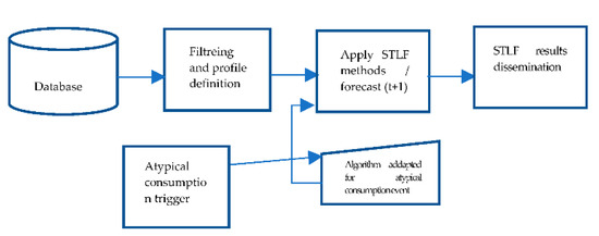
Figure 1.
Flowchart of STLF in atypical consumption behavior.
2. Database Presentation
The database is a representative sample of both rural (7k households) and urban consumers (23k households). The database is a multiannual (2019–2021) recording of hourly energy use and is provided as Supplementary Material to this manuscript. Due to the volume of information to disseminate in this paper, we approach all the specifications and particularities of the database that are essential to this research. The urban households are located in cities in Bihor County, Romania, in the second climatological area, with an annual average temperature of 11.6 °C [15]. We present three charts specific to the yearly average urban database. Figure 2 shows the yearly consumption relative to 2020, the year for which we have the atypical consumption behavior that we targeted in our STLF deployment. Figure 3 shows the weekday consumption and Figure 4 the seasonal profile consumption. For profiling reasons, Figure 2 presents only 2020 data, but Figure 3 and Figure 4 statistically address all three years covered by the database. The rural households are located in Bihor County, Romania, in the third climatological area, with an annual average temperature of 9.6 °C [16]. In Figure 5 we can see a representative chart of the 2020 yearly consumption segmented into weekly loads starting on Sundays. Figure 6 and Figure 7 show the statistics of the specific consumption of the rural household over weekdays and over each season.
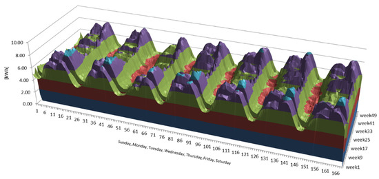
Figure 2.
Weekly load curve in 2020 for urban consumers.
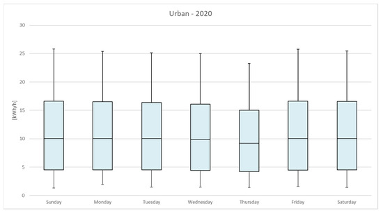
Figure 3.
Box and whiskers plots for days of the week in 2020 (urban).
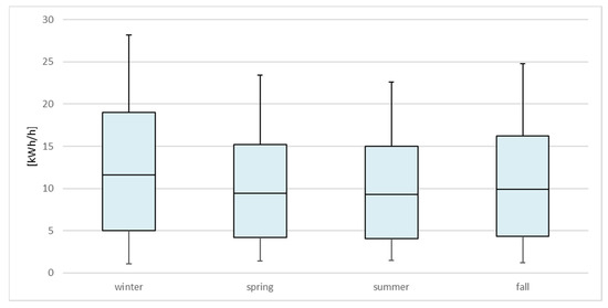
Figure 4.
Box and whiskers plots for hourly consumption in each season in 2020 (urban).
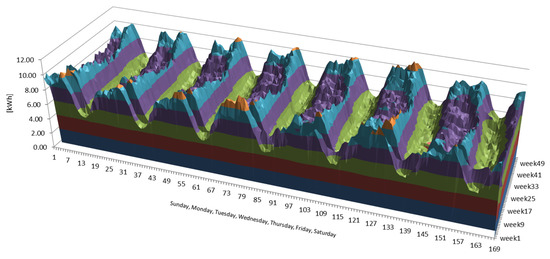
Figure 5.
Weekly load curve in 2020 for rural consumers.
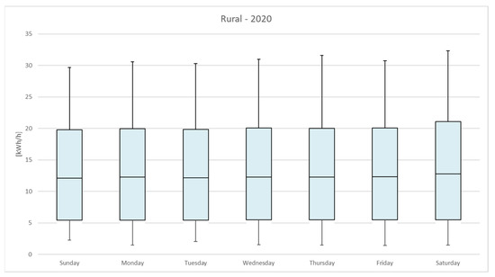
Figure 6.
Box and whiskers plots for days of the week in 2020 (rural).
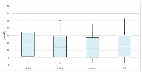
Figure 7.
Box and whiskers plots for hourly consumption in each season in 2020 (rural).
Although weekly patterns are rare in nature, they are common in human activities, which is why we chose a 3D yearly chart; this chart contains essential information for classifying the consumption pattern.
The weekday pattern for urban residential consumers in Bihor County (RBCR) was relatively similar to the weekday patterns in Ireland, Hungary, Italy and UK, with the caveat that the household electric energy consumption was different [17]. With regard to the daily high peaks, the urban RBCR consumer was closer to the consumer profile from Hungary and Italy than that from Ireland and the UK [17].
In comparing the weekday consumption for rural and urban RBCR, the differences were due to the specific activities that take place in rural areas (Figure 8). While the urban consumption on weekdays (Monday to Friday) showed a bell shape, the rural chart showed a flattened reversed bell. While the most active days in terms of electric energy consumption seemed to take place on Wednesdays in the urban areas, in the rural ones the highest consumption was associated with Fridays [14].
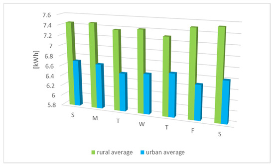
Figure 8.
Rural vs. urban weekly consumption patterns.
The weekend daily consumption pattern was relatively similar for urban and rural consumers in the regard that the consumption was lower on Saturday and higher on Sunday. The increase in Sunday consumption was bigger for the urban RBCRs. The same load profile was seen in all other countries’ consumers that were analyzed [17] with a higher consumption on Sunday vs. Saturday [14].
A particularity of the rural RCBR is that it stands out of the large EU patterns identified in previous studies [17], with less consumption on Saturday relative to Friday. This particularity could be a good asset in forecasting and deploying power network resources.
With regard to the meteorological season’s consumption pattern, we can see that the county is similar to the other EU countries covered so far in previous studies [17] with a good correlation with the day degree influence factor. The seasonal consumption pattern was more closely related to that of Italy and Hungary than that of Ireland and the UK [14].
The gap in summer consumption in seasonal analysis was steeper for the rural RBCR consumers (Figure 9). We associate this finding with a poor penetration of air-conditioning cooling devices in rural areas. In addition, in comparison to previous studies [17], we can see that this consumption was increased in the winter not due to electrical heating but mainly to the lower availability of natural light and the movement of activities indoors.
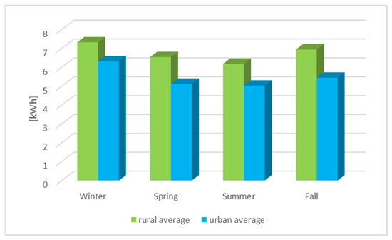
Figure 9.
Rural vs. urban meteorological season consumption patterns.
The differences in consumption patterns could be connected to energy-related education levels [18] and with poor market availability of smart meters and hourly billing for RBCRs.
In previous research [2] we found that identifying, analyzing and clustering consumer types can have a very good outcome in modeling and forecasting short-term and medium-term power consumption. These findings have implications in assessing and developing commercial electric energy prices.
The database used in this study was extracted from a public national database [19].
3. Methodology
Although most of the research on load forecasting is on advance forecasting techniques, decision-making revolves around classical forecasting methods: moving average, linear regression and multiple linear regression [20]. We assess three methods of forecasting for atypical consumption behavior: linear regression (LR), autoregressive integrated moving average (ARIMA) and Artificial Neural Network (ANN). Previous estimations performed with fuzzy forecasting methods gave high errors [21], so we did not include fuzzy forecasting in this study.
The first steps were digesting the database and preparing it for deeper understanding and ease of mathematical modeling. Influence factor databases were also added and filtered, including the weather database and the weekly and daily databases containing socio-cultural and economic activity milestones. The database was a fixed one, and none of the methods used was trained to update in real time with an expanding database.
3.1. Database Filtering for Outlier Values and Noise Removal
A relatively simple filter to remove outlier values was constructed. The limit of the outlier value was stated at six times the mean value. First, 25 outlier values in each database were double-checked and manually confirmed [14,22,23].
where:
- x is the actual value,
- m is the mean value.
3.2. Correlation of Database Values with the Exterior Influence Factors
We used a standard correlation model for a yearly database [2]:
where x is the actual power database value and is the average of similar temporal values, e.g., same time interval of the same day of the week in the same season; y is the actual meteorological/daylight database value and is the average of similar temporal values.
3.3. Linear Regression
The first forecasting in each line of estimation was carried out with the industry’s most commonly used method [20]:
where:
- y(t) is value at time t to be forecasted;
- x1(t) represents the influence factors;
- r(t) is the residual load at t;
- ai is the regression parameter.
3.4. Autoregressive Integrated Moving Average
Having a proven higher efficiency in forecasting data highly related with human activities and behavior [24,25], we used as the second forecasting method the ARIMA technique:
where:
- Xt represents the time series data;
- αi represents the parameters of the autoregressive part of the model;
- θi represents the parameters of the moving average part;
- εt is the error term.
3.5. Artificial Neural Network
Available on a large scale and easy to train and use, the ANN method is the first weapon of choice after regression techniques. We used a multilevel ANN (feed forward) including gradient descent and backpropagation algorithms by minimizing error with a non-Euclidean-type function. Multilevel feed forward networks are trained via supervised methods involving the use of training instances of the form (Xp, tp)
- Xp = (Xp1, Xp2, …, XpN ) is the input vector for the training p;
- tp = (tp1, tp2, …, tpM ) is the desired output vector for p;
- N is the number of input units of the network;
- M is the number of output units.
If F(X) is the function processing the problem as per input X:
then the output by processing the input data using neural network is defined by:
where Op is the result of processing of the input, Xp, by using the function Fw(w;Xp) network applied as an approximation of F(X), so:
tp = F(Xp)
Op = (Op1, Op2, …, OpM)
Op = Fw(w;Xp)
The error recorded during processing through the network of the input vector Xp—i.e., the measured error in a unit of output Uj—defined by is expressed as the difference between desired and actual output achieved:
ejp = tjp − Ojp
Error Ep, recorded during the processing through the network of the input vector Xp and established across the whole neural network, is obtained by combining the error based on a relationship of the form:
For error calculation the Ep error and zero based log sigmoid function are used:
3.6. Forecasting Error Assesing with Mean Absolute Percentage Error (MAPE)
Usually, the assessment of forecasting errors is conducted with two or three indicators, such as Mean Absolute Error (MAE) and MAPE of Root Mean Square Error (RMSE), but taking into consideration that the average values for rural and urban consumption per household differed significantly [14] we used only the MAPE to evaluate forecasting method accuracy.
where Pi is the power value at time I, is the forecasted power value for time i and N is the number of the forecasted value.
3.7. Trigger/Alarm for Atypical Consumption Behavior in Near Future
An unpredictable and unexpected event that is related to human behavior as consumption has very limited available information that can be used in forecasting [26,27].
We assume that such an event will not be visible prior to occurrence in available databases. Therefore, we must rely on big data analytics [28] and identify a threshold using methods other than the Twitter analytics proposed in [28] that can raise the alarm for the next STLF. Behind every forecast, there is a human operator that makes sure the database is delivered correctly, and this method would first check the assumptions that are made. Knowing that all human activities are subject to error, we must try to deploy an automatic trigger that raises an alarm based on an explosion of breaking news, such that the human operator could address this alarm and decide if action is needed or if the forecast should be deployed as before [29,30].
3.8. Steps to Identify the Best Forecasting Method under Atypical Consumer Behavior
The recommended way to address a forecast, and afterwards forecast under atypical behavior, is stated hereunder:
- Database presentation, including specific, known influence factors;
- Database filtering, denoising and outlier value removal;
- Identification of sensitivity of consumer behavior to influence factors (weather, socio-economic activities, etc.) by correlation;
- Deploying multiple forecasting algorithms and identifying the most accurate one for the specific database;
- Setting up a trigger/alarm for future atypical consumption behavior;
- Deploying forecasting methods adapted for the atypical event;
- Identifying best practices and disseminating them.
All these steps should take into consideration that each database has its particularities, and these steps should address each and every one of them, e.g.: one deployment for weekdays and a separate one for weekend days, separate deployments for winter and summer, etc.
4. Case Analysis
Applying the steps mentioned in Section 3.8, the returned results were as follows:
- The few outlier values identified were removed by the filtering algorithm.
- The database had high fidelity and we encountered few outlier values, under 0.02% (0 or close to 0, or unusually high, more than six times the load peak value);
- We assessed the correlation between the influence factors, mainly weather and socio-cultural events, and consumption among rural consumers to be r = −0.2797 versus that among urban consumers, r = −0.2651;
- In order to validate the correlation results we clustered the database by weekdays, one profile for each weekday, to identify characteristics and compare with similar consumption in the EU [17]. Clustering was also performed for meteorological seasons for the above-mentioned comparison;
- The overall short-term load forecast (STLF) was performed over 2020 day by day, using the above-mentioned algorithms, and the results are described in the box and whiskers BW charts in Figure 10 for rural and Figure 11 for urban consumers. This forecast was carried out not taking into consideration the influence of the COVID-19 restrictions and lockdowns, just the usual influence factors and historic data.
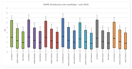 Figure 10. Overall forecasting results for rural consumers in 2020.
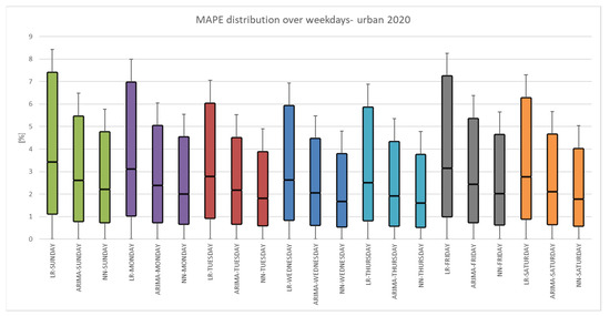 Figure 11. Overall forecasting results for urban consumers in 2020.
 - Examining the forecast for the first day of lockdown without any correction to the algorithm, we encountered very high values of MAPE, as shown in Table 1 and in Figure 12 and Figure 13. Using the atypical consumer behavior alarm trigger, we could increase the forecast accuracy by altering the algorithm, as shown in Table 2, by adding weekend parameters—a combination of morning Saturday and afternoon Sunday—for the first weekday of lockdown; the first day of the lockdown in Bihor County, Romania, was a Tuesday, and as we say in Eastern Europe, Tuesday—three times bad luck [31]. This day provided a mix of bad luck and opportunity for power market participants and for the power grid operating personnel;
 Table 1. MAPE results using the unaltered STLF algorithm.
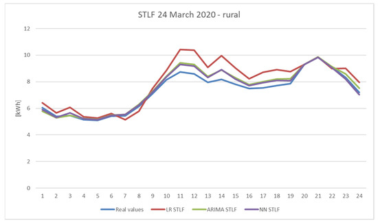 Figure 12. STLF results for 24th March 2020—rural consumers without the adapted algorithm.
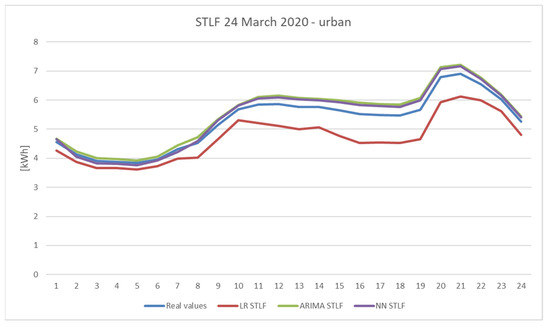 Figure 13. STLF results for 24th March 2020—urban consumers without the adapted algorithm.
Table 2. MAPE results using the adapted STLF algorithm (TRIGGER ON).
Figure 13. STLF results for 24th March 2020—urban consumers without the adapted algorithm.
Table 2. MAPE results using the adapted STLF algorithm (TRIGGER ON). - The effects of the second and subsequent lockdowns did not have such a big impact on the forecast accuracy relative to the preceding history of power load; the MAPE results were almost similar to a common forecast.
5. Discussion
As all the STLF literature states, a deep understanding of the consumers analyzed or of the database modeled is critical in forecasting under atypical consumer behavior [18,32] or under power load black swan events [26].
The analyzed database was composed of multiyear data from rural (7k households) and urban consumers (23k households) in Bihor County, Romania and we managed to identify the social, economic and weather influence factors. The database contained nonresidential consumers at levels that did not influence the residential patterns, including small and medium enterprises (SME).
During this study, we found large gaps between the unaltered STLF algorithm and algorithms adapted to atypical consumption or unforeseen events.
Previous studies [3,4,5,6,7] focused on algorithms for predicting outcomes with no historical database for a comparable situation. We tried to highlight the fact that for each unforeseen power load event or atypical behavior pattern, we should adapt the algorithm individually for each scenario. If for COVID-19 lockdown there was an easy fix, as the weekend historical consumption could be easily applied to all of the methods proposed, for other unforeseen events that cause atypical consumption behavior we need to identify scenarios and trends.
We plan to broaden our area of research by covering power load consumption unforeseen events at different layers of social, educational and economic levels and by analyzing different databases that encountered unforeseen events, e.g., the February 2021 Texas blackout, February 2014 Ukraine War, February 2020 market crash, 2021 global and European energy crisis, etc. As future research projects we aim to identify historical power load data that are related to unforeseen events and use them as a load forecast “library” for atypical consumption behavior as a cause of such events.
Regardless of the future conditions and state of the pandemic, its impact should be further studied in regard to the medium- and long-term load forecast (MTLF and LTLF), as COVID-19 more significantly affected other social and economic areas that have a relatively large impact on power consumption. Only working from home and online education, which prior to COVID-19 were merely exceptional cases, will become standard activities that might have a major impact on residential load consumption.
6. Conclusions
The three methods applied were deployed in a short period of time. The hardware configuration of the machine that generated the forecasts included 8 GB RAM, 500 GB SSD and an i5 Intel Processor. The LR and ARIMA methods were easy to use and adjust and could be modeled and tuned in Excel [14] (Microsoft Office 2019). For the ANN method R Statistics software’s CRAN package was used. All analyzed methods output a good response to the influence factors with a retardation of one measurement or production data. We are certain that if a database of meteorological data collected from the immediate vicinity were available, we could increase the forecasting methods’ accuracies by at least 0.5% (MAPE) for standard consumption data. The ANN method results, for this particular database, did not significantly improve after 100 epochs during the training process. The best results were obtained with seven hidden layers and 10 neurons in each hidden layer.
As we had available multiple metrics to evaluate our forecast, we used only MAPE because there was a significant difference between rural and urban household consumption (kWh) with an approximately 20% larger consumption in rural households.
The high reduction in MAPE of residential consumption on the first day of lockdown in Bihor County, Romania when the algorithm was adapted for the atypical consumption justifies the importance of this study; we had an overall MAPE = 4.0071% compared to the adapted algorithm MAPE = 1.4152%. This almost 3% difference in accuracy could have major economic effects on participants on the energy market. In [3] the results from the same country, but including a database that also contained commercial and industrial consumers, were relatively similar (MAPE) for the model adapted for pandemic effects, but our unadapted forecast method had a 2% to 3% higher MAPE. We conclude that residential consumers are highly sensitive to unforeseen events. We intend to focus our future research on a trigger algorithm that could automatically flag unforeseen events and atypical consumption behavior. This future focus may cover an algorithm for identifying an increase in information shared via social media related to energy consumption and its impact on the load curve, and use this to define the trigger to flag atypical or unforeseen power load consumption events. Also we intend to identify the influence of the level of education [33] and energy education in the power consumption response to atypical events.
Supplementary Materials
The following supporting information can be downloaded at: https://www.mdpi.com/article/10.3390/en15010291/s1.
Author Contributions
Conceptualization, F.C.D. and C.H.; methodology, F.C.D. and C.S.; software, F.C.D.; validation, C.H. and G.B.; formal analysis, C.S.; investigation, F.C.D.; resources, C.H.; data curation, F.C.D.; writing—original draft preparation, F.C.D.; visualization, C.H., G.B. and C.S.; supervision, C.H.; funding acquisition, C.H. All authors have read and agreed to the published version of the manuscript.
Funding
This research received no external funding.
Institutional Review Board Statement
Not applicable.
Informed Consent Statement
Not applicable.
Data Availability Statement
Not applicable.
Acknowledgments
Not applicable.
Conflicts of Interest
The authors declare no conflict of interest.
Abbreviations
| ANN | artificial neural network |
| ARIMA | autoregressive integrated moving average |
| ARIMAX | Autoregressive Integrated Moving Average with Exogenous |
| CNN | convolutional neural network |
| EU | European Union |
| FCDNN | Fully Connected Deep Neural Network |
| GAM | Generalized Additive Models |
| GRU | Gated Recurrent Unit |
| LR | linear regression |
| LSTM | Long Short-Term Memory |
| LTLF | long-term load forecast |
| MAE | Mean Absolute Error |
| MAPE | Mean Absolute Percentage Error |
| MLR | multiple linear regression |
| MTLF | medium-term load forecast |
| NEPCO | National Electric Power Company |
| NY | New York |
| PJM | Pennsylvania, New Jersey, Maryland |
| RCBR | residential consumers in Bihor County, Romania |
| RMSE | Root Mean Square Error |
| SME | small and medium enterprise |
| SOM | system operator method |
| STLF | Short-term load forecasting |
| UK | United Kingdom |
| US | United States |
References
- Felea, I.; Goude, Y.; Dan, F. Electric energy forecast for the industrial consumers using neural network. J. Sustain. Energy 2011, 2, 89–94. [Google Scholar]
- Felea, I.; Dan, F.; Dzitac, S. Consumers load profile classification corelated to the electric energy forecast. Proc. Rom. Acad. Ser. A 2011, 13, 80–88. [Google Scholar]
- Tudose, A.M.; Picioroaga, I.I.; Sidea, D.O.; Bulac, C.; Boicea, V.A. Short-Term Load Forecasting Using Convolutional Neural Networks in COVID-19 Context: The Romanian Case Study. Energies 2021, 14, 4046. [Google Scholar] [CrossRef]
- Wang, Z.; Hao, W. Improving Load Forecast in Energy Markets during COVID-19; Association for Computing Machinery: New York, NY, USA, 2021. [Google Scholar] [CrossRef]
- Alasali, F.; Nusair, K.; Alhmoud, L.; Zarour, E. Impact of the COVID-19 Pandemic on Electricity Demand and Load Forecasting. Sustainability 2021, 13, 1435. [Google Scholar] [CrossRef]
- Kozak, D.; Holladay, S.; Fasshauer, G. Intraday Load Forecasts with Uncertainty. Energies 2019, 12, 1833. [Google Scholar] [CrossRef] [Green Version]
- Obst, D.; Vilmarest, J.; Goude, Y. Adaptive Methods for Short-Term Electricity Load Forecasting During COVID-19 Lockdown in France. IEEE Trans. Power Syst. 2021, 36, 4754–4763. [Google Scholar] [CrossRef]
- COVID-19 Pandemic in Romania. Available online: https://en.wikipedia.org/wiki/COVID-19_pandemic_in_Romania (accessed on 21 November 2021).
- Romania Announces Nationwide Lockdown Measures to Limit Spread of COVID-19. Available online: https://www.garda.com/crisis24/news-alerts/326626/romania-government-announces-lockdown-measures-on-march-25-update-2 (accessed on 21 November 2021).
- Press Releases—Health Ministry—Bihor County Public Health Department. Available online: http://www.dspbihor.gov.ro/comunicatedepresa2020.html (accessed on 21 November 2021).
- Press Releases—Bihor County Prefect Institution—Internal Affairs Ministry. Available online: https://bh.prefectura.mai.gov.ro/category/comunicate-de-presa/ (accessed on 21 November 2021).
- One Corovanirus, 28 States: A Comparison of Anti-Covid-19 Measures Decided in Each EU Member State. Available online: https://cursdeguvernare.ro/tari-diferite-restrictii-diferite-o-comparatie-a-masurilor-anti-covid-19-decise-in-fiecare-stat-membru-ue.html (accessed on 21 November 2021).
- Bihor County Population Assessment at 1 January 2020—INS—BIHOR County Statistics Department. Available online: https://bihor.insse.ro/wp-content/uploads/2020/05/Populatia-BH-la-1-ianuarie-2020.pdf (accessed on 21 November 2021).
- Dan, F.C.; Hora, C.; Gligor, E.; Majoros, N.T. Identification of Load Profiles for Rural and Urban Consumers in Bihor County, Romania. In Proceedings of the National Technical Scientific Conference, “Modern Technologies for the 3rd Millenium”, 20th ed.; Editografica: Bologna, Italy, 2021. [Google Scholar]
- Dumiter, A.F. Climate and Topoclimates of ORADEA. Ph.D. Thesis, University of Oradea, Oradea, Romania, 2007. [Google Scholar]
- National Technical Standard: Order No. 386/2016 for Modification and Completing of Technical Reglementation “Normative Regarding the Thermotechnical Calculation of the Construction Elements of the Buildings”, Indicative C 107-2005. Available online: http://www.stim.ugal.ro/crios/Support/IEACA/Anexe/C107-1-3-2005.pdf (accessed on 21 November 2021).
- Kmetty, Z. Load Profile Classification, WP4—Classification of EU Residential Energy Consumers. Technical Public Report, January 2016. [Google Scholar] [CrossRef]
- Kiss, J.F. Educational Policies in Relation to Society. Stud. Teach. J. Teach. Train. Educ. Res. 2020, 1, 43–50. [Google Scholar]
- Transelectrica—Consumption Chart. Available online: https://www.transelectrica.ro/en/widget/web/tel/sen-grafic/-/SENGrafic_WAR_SENGraficportlet (accessed on 21 November 2021).
- Top Four Types of Forecasting Methods. Available online: https://corporatefinanceinstitute.com/resources/knowledge/modeling/forecasting-methods/ (accessed on 21 November 2021).
- Dan, F.C.; Hora, C.; Bendea, G. Short-Term Forecasting of Wind Power Generation. In Proceedings of the 2021 10th International Conference on ENERGY and ENVIRONMENT (CIEM), Bucharest, Romania, 14–15 October 2021. [Google Scholar]
- Xiong, H.; Pandey, G.; Steinbach, M.; Kumar, V. Enhancing data analysis with noise removal. IEEE Trans. Knowl. Data Eng. 2006, 18, 304–319. [Google Scholar] [CrossRef] [Green Version]
- Guo, G.; Wand, H.; Bell, D. Data Reduction and Noise Filtering for Predicting Times Series. In Proceedings of the Advances in Web-Age Information Management, Third International Conference, Beijing, China, 11–13 August 2002. [Google Scholar] [CrossRef]
- Sabry, M.; Badra, N. Comparison Between Regression and Arima Models in Forecasting Traffic Volume. Aust. J. Basic Appl. Sci. 2007, 1, 126–136. [Google Scholar]
- ARIMA Compared to Linear Regression, Introduction to Trading, Machine Learning & GCP, Online Video Course. Available online: https://www.coursera.org/lecture/introduction-trading-machine-learning-gcp/arima-compared-to-linear-regression-ZxJ11 (accessed on 21 November 2021).
- Taleb, N.N. The Black Swan: The Impact of the Highly Improbable, 2nd ed.; Random House: New York, NY, USA, 2007. [Google Scholar]
- Tan, L. The Mandelbrot Set, Theme and Variations; Cambridge University Press: Cambridge, UK, 2000; ISBN 978-0-521-77476-5. [Google Scholar]
- Ali, Y. A Proposed Framework for Predicting Emergency Events Using Big Data Analytics. Ph.D. Thesis, Helwan University, Cairo, Egypt, 2021. [Google Scholar]
- Lazer, D.; Baum, M.; Grinberg, N.; Friedland, L.; Joseph, K. Combating Fake News: An Agenda for Research and Action, Harvard Kennedy School, Northeastern University, 2017, US. Available online: https://apo.org.au/sites/default/files/resource-files/2017-05/apo-nid76233.pdf (accessed on 21 November 2021).
- Conneau, A.; Schwenk, H.; Barrault, L.; Lecun, Y. Very Deep Convolutional Networks for Text Classification. arXiv 2016, arXiv:1606.01781. Available online: https://arxiv.org/pdf/1606.01781.pdf (accessed on 21 November 2021).
- Tuesday 13: Romania Tops Europe’s Superstition Charts. Available online: https://www.romania-insider.com/tuesday-13-unlucky-for-some (accessed on 21 November 2021).
- Blaga, A.C.; Gligor, E. Monoagent heating systems for solitary consumers. J. Appl. Eng. Sci. 2011, 2, 36–42. [Google Scholar]
- Dan, B.A.; Kovàcs, K.E. The Link between Experiential Pedagogy and Community Schools in Community Building and Social Innovation; Boros, J., Kozma, T., Markus, E., Eds.; Debrecen University Press: Debrecen, Hungary, 2021; pp. 12–25. ISBN 978-963-318-943-6. [Google Scholar]
Publisher’s Note: MDPI stays neutral with regard to jurisdictional claims in published maps and institutional affiliations. |
© 2022 by the authors. Licensee MDPI, Basel, Switzerland. This article is an open access article distributed under the terms and conditions of the Creative Commons Attribution (CC BY) license (https://creativecommons.org/licenses/by/4.0/).