Model Reference Tracking Control Solutions for a Visual Servo System Based on a Virtual State from Unknown Dynamics

Abstract

This paper focuses on validating a model-free Value Iteration Reinforcement Learning (MFVI-RL) control solution on a visual servo tracking system in a comprehensive manner starting from theoretical convergence analysis to detailed hardware and software implementation. Learning is based on a virtual state representation reconstructed from input-output (I/O) system samples under nonlinear observability and unknown dynamics assumptions, while the goal is to ensure linear output reference model (ORM) tracking. Secondary, a competitive model-free Virtual State-Feedback Reference Tuning (VSFRT) is learned from the same I/O data using the same virtual state representation, demonstrating the framework’s learning capability. A model-based two degrees-of-freedom (2DOF) output feedback controller serving as a comparisons baseline is designed and tuned using an identified system model. With similar complexity and linear controller structure, MFVI-RL is shown to be superior, confirming that the model-based design issue of poor identified system model and control performance degradation can be solved in a direct data-driven style. Apart from establishing a formal connection between output feedback control, state feedback control and also between classical control and artificial intelligence methods, the results also point out several practical trade-offs, such as I/O data exploration quality and control performance leverage with data volume, control goal and controller complexity.

1. Introduction

The reinforcement learning (RL) paradigm has seen significant recent development in terms of both artificial intelligence (AI) and in control systems as the two main paths leading the research, with some of the most popularized achievements belonging to the former area. However, recent progress has seen hybridization of ideas from the two fields. The promise of data-driven RL is its ability to learn complex decision policies (controllers) under uncertain, unknown (model-free), high-dimensional environments. While the AI approach largely deals with scalability issues, learning efficiency in terms of data volume and speed, and complex environments, some other features are also well-established, such as, e.g., using neural networks (NNs) (plain feedforward, convolutional or LSTM-like recurrent ones) as function approximators, both for the value function and for the policy function, which is the golden standard. The AI approach presents many contributions, such as parallel exploration using multiple environments to enrich exploration diversity, or sparse or dense reward-shaping in various environments under hierarchical learning problem formulation [1,2], and value function overestimation biasing the learning in random environments, which is dealt with by multiple value function approximators, different update frequencies of the critic and policy networks, target policy smoothing, etc., in DDPG, TD3 and SAC versions [3,4,5], to name a few.

But it should be of no surprise that most of these RL achievements in AI have been tested under simulation environments, like video games (DQN Atari for example) and other simulated mechatronics, and not in real world test rigs. In the context of real-world control problems other issues prevail, such as: stability and learning convergence meet the learning efficiency in terms of data volume, and mechanical constraints and real-time implementation requirements being leveraged by efficient function approximators. This is the reason why classical control theory has addressed RL control from somewhat different perspectives than AI. In addition, real-world control problems have often and traditionally been considered as low-dimensional compared to AI problems.

Some of the earliest works in RL, also known as approximate (adaptive) dynamic programming, have been established by seminal works of [6,7,8]. RL for control uses two main algorithms, namely Policy Iteration (PoIt) and Value Iteration (VI), and their in-between, Generalized PoIt [7]. In the context of these two popular RL algorithms, the implementation flavors have witnessed offline and online variants, batch- and sample-by-sample adaptive-wise, model-based and model-free, and their combinations. Out of the two algorithms, VI-RL has been arguably considered as the most attractive, since it spans the “unknown dynamics” control case, and its initial controller and value function approximators bear random initialization, which is natural when unknown system dynamics are assumed from start. A significant effort was dedicated to ensuring learning convergence and stability, more generally under generic function approximators, such as NNs.

Much of the learnability in RL relies on the Markovian assumption about the controlled system, together with its full state availability. Although different state representations have been proposed in AI, involving virtual states (called state aliases) built from present and past system’s input-output (I/O) data samples, it has not benefited from a well-established theoretical foundation [9]. However, for RL in control systems, the system observability and controllability are well-founded concepts from a historical perspective [10,11].

Among the vast practical control problems approached by RL under classical control analysis approach [12,13,14,15,16,17] and under AI-based analysis approach [18,19,20,21], the output reference model (ORM) tracking has attracted a lot of research attention [12,22,23,24]. This control problem tries learning a state-feedback controller to make the controlled system output behave similarly to the ORM’s output, under the same reference input excitation signal. The practical implications of ORM tracking are even more appealing when linear ORMs are used, as indirect feedback linearization is ensured, i.e., a nonlinear system coupled with a nonlinear controller to make the closed-loop control system (CLS) match a linear ORM. Such control problem can be posed as an optimal control problem and has been solved, e.g., by VI-RL and Virtual State-Feedback Reference Tuning (VSFRT) control learning approaches [24]. This linear ORM tracking has proven itself as the building block for more advanced hierarchical control architectures [25,26] aimed at generalizing learned optimal tracking behavior to new unseen trajectories, therefore endowing control systems with extrapolation reasoning similar to intelligent beings. Such goals have been tackled by primitive-based learning frameworks [25,26,27,28,29,30].

Learning LORM tracking control from system I/O data samples with unknown dynamics based on a virtual state representation is a data-driven research approach motivated by the need to solve the control performance degradation occurring due to the mismatch between the true, complex system and its identified, simplified and uncertain model. This is considered a nuisance with the model-based control paradigm. In this context, this work’s contribution is threefold:

(a)

a novel convergence analysis of the model-free VI-RL (MFVI-RL) algorithm is proposed. The iterative convergence of the cost function towards the optimal cost and the convergence of the iterative controller towards the optimal controller are proven, as updated by VI steps;

(b)

an original validation on a visual servo tracking system comprising of an inexpensive and modern hardware processing platform (Arduino) combined with the software platform MATLAB. The visual tracking control validation uses the new state representation comprising of present and past I/O data samples;

(c)

the proposed MFVI-RL (implemented with NN approximator for the Q-value function and with linear controller parameterization) is compared with:

(1)

a model-based control strategy aiming at the same objective, namely a two-degree-of-freedom (2DOF) controller for ORM tracking; and

(2)

with a competitive VSFRT linearly parameterized controller also sharing the same learning control objective and the same underlying virtual state representation.

The learning process for MFVI-RL and VSFRT utilizes a form of pseudo-state-feedback control where, in fact, I/O data is used only for reconstructing the virtual state.

The paper is organized as next presented. Section 2 deals with VI-RL convergence under general assumptions. Section 3 integrates several subsections, such as: the visual servo system hardware and software description, followed by the LORM tracking problem formulation, subsequently solved by 2DOF control, by VI-RL algorithm and by VSFRT algorithm. All three are presented in detail. Performance comparisons reveal the learned control performance and offer the achieved results’ interpretation.

2. The VI-RL Convergence Analysis for ORM Tracking Systems

The VI-RL convergence analysis is first performed in terms of the original “V” cost function, for ORM tracking systems for which particular penalty functions are sought. The result is then straightforwardly extended to the case of extended “Q” cost function, which characterizes the subsequent MFVI-RL implementation where the controlled system is assumed with unknown dynamics. Furthermore, the derivations are based on a state-space model, however this will be relaxed later on since a new state-space representation is reconstructed from I/O system data samples, using the virtual state transformation concept. Which implies that from any I/O nonlinear unknown dynamics system model which is assumed to be observable, we could arrive at a state-space model, with unknown dynamics a but measurable state. This will be clearly illustrated in the validation case study. For now, let the nonlinear unknown state-space system be

$$\{\begin{array}{c}{\mathit{s}}_{k+1}=\mathit{f}\left({\mathit{s}}_k,{\mathit{u}}_k\right),\\ {\mathit{y}}_k=\mathit{h}\left({\mathit{s}}_k\right),\hfill \end{array}$$

(1)

defined in discrete-time, comprising of a transition function equation and an output equation, respectively. The system state is ${\mathit{s}}_k={[s_{k,1}\dots s_{k,n}]}^T\in {\Omega }_S\subset {\Re }^n$, the system’s input is ${\mathit{u}}_k={[u_{k,1},\dots ,u_{k,m_u}]}^T\in {\Omega }_U\subset {\Re }^{m_u}$, and the measured (and controlled) output is denoted as ${\mathit{y}}_k={[y_{k,1},\dots ,y_{k,p}]}^T\in {\Omega }_Y\subset {\Re }^p$. The functions $\mathit{f},\mathit{h}$ are assumed as unknown on their definition domains and also continuously differentiable.

The cost function to be minimized is the summed penalties over an infinite horizon, which reduces to the control problem

$$\begin{gathered} C^{*}=arg\underset{C}{min}V\left({\mathit{s}}_k\right)={\displaystyle \sum }_{i=k}^{\infty }\mho \left({\mathit{s}}_i,{\mathit{u}}_i\right), \\ \mathrm{s}.\mathrm{t}. {\mathit{u}}_i=C\left({\mathit{s}}_i\right), \end{gathered}$$

(2)

where $\mathsf{\mho }\left({\mathit{s}}_i,{\mathit{u}}_i\right): {\Omega }_S\to {\Re }^n$ is the penalty function which is dependent only on ${\mathit{s}}_i$, and has the property that $\mathsf{\mho }\left({\mathit{s}}_i,{\mathit{u}}_i\right)\ge 0$, $\forall {\mathit{s}}_i\in {\Omega }_S, \forall {\mathit{u}}_i\in {\Omega }_U$. The penalty function has the value $\mathsf{\mho }\left({\mathit{s}}_i,{\mathit{u}}_i\right)=0$ only when ${\mathit{s}}_k={\mathit{s}}_{\mathbf{G}}$, with ${\mathit{s}}_{\mathbf{G}}$ some goal (or target) state.

Observation 1. In the case of linear quadratic control, the penalty function is commonly $\mathsf{\mho }\left({\mathit{s}}_i,{\mathit{u}}_i\right)={\mathit{s}}_i^T\mathbf{Q}{\mathit{s}}_i+{\mathit{u}}_i^T\mathbf{R}{\mathit{u}}_i$ with respect to regulation of the system state towards zero. Here, $\mathbf{Q}\ge 0$ and $\mathbf{R}>0$ are positive definite penalty matrices on the state energy and on the control input energy, respectively. It is known that the missing input energy penalization (for $\mathbf{R}=0$) renders the linear optimal control unfeasible. In the case of ORM tracking systems where the time-varying goal state is the result of a reference model dynamic system, it is possible to define a penalty function independent on the control input energy, e.g., as in $\mathsf{\mho }\left({\mathit{s}}_i,{\mathit{u}}_i\right)={\left({\mathit{s}}_i-{\mathit{s}}_{\mathbf{G}}\right)}^T\mathbf{Q}\left({\mathit{s}}_i-{\mathit{s}}_{\mathbf{G}}\right)$. This would eventually lead to a feasible optimal control solution. We preserve notation $\mathsf{\mho }\left({\mathit{s}}_i,{\mathit{u}}_i\right)$ even if there is no explicit dependence on ${\mathit{u}}_i$ since this will prove to be useful when acknowledging the role of the control input ${\mathit{u}}_i$ in transiting from one state ${\mathit{s}}_k$ to another one ${\mathit{s}}_{k+1}$.

Let $V^{*}\left({\mathit{s}}_k\right)$ and $C_j^{*}\left({\mathit{s}}_k\right)$ be the optimal cost and the optimal controller. In the following, $\underset{\mathit{u}}{min}\{.\}$ and $\underset{C}{min}\{.\}$ will imply the same operation under the constraint that $\mathit{u}=C\left(\mathit{s}\right)$. Starting with an initial controller $C_0$ and V-function $V_0\left({\mathit{s}}_k\right)=0$, for all possible combinations of $\left({\mathit{s}}_k,{\mathit{u}}_k\right)$, $C_0\left({\mathit{s}}_k\right)$ is solved as follows:

$$C_0\left({\mathit{s}}_k\right)=arg\underset{\mathit{u}}{min}\left\{\mathsf{\mho }\left({\mathit{s}}_k,\mathit{u}\right)+V_0\left({\mathit{s}}_{k+1}\right)\right\}=arg\underset{\mathit{u}}{min}\left\{\mathsf{\mho }\left({\mathit{s}}_k,\mathit{u}\right)\right\}.$$

(3)

Having the policy determined, the c.f. update renders

$$V_1\left({\mathit{s}}_k\right)=\mathsf{\mho }\left({\mathit{s}}_k,C_0\left({\mathit{s}}_k\right)\right)+V_0\left({\mathit{s}}_{k+1}\right).$$

(4)

Then, for the iterative VI algorithm the following steps are alternated at each j-th iteration:

S1. Update the controller

$$C_j\left({\mathit{s}}_k\right)=arg\underset{\mathit{u}}{min}\left\{\mathsf{\mho }\left({\mathit{s}}_k,\mathit{u}\right)+V_j\left({\mathit{s}}_{k+1}\right)\right\}.$$

(5)

S2. Update the V-function

$$V_{j+1}\left({\mathit{s}}_k\right)=\mathsf{\mho }\left({\mathit{s}}_k,C_j\left({\mathit{s}}_k\right)\right)+V_j\left({\mathit{s}}_{k+1}\right) .$$

(6)

Assumption 1.

We assume that the system is fully state controllable. This means that any state ${\mathit{s}}_k\subset {\Omega }_S$ can be accessed from any other initial state in a finite number of time steps.

Assumption 2.

We assume all the states from the process have been uniformly visited, and each possible action was tried for each possible state. This is equivalent to a complete fully state exploration, that reveals all the process dynamics.

Definition 1.

The transition distance $d\left({\mathit{s}}_k,{\mathit{s}}_{\mathbf{G}}\right)=\varpi$ is defined as the number $\varpi$ of minimum state transitions from ${\mathit{s}}_k$ to ${\mathit{s}}_{\mathbf{G}}$ using a succession of commands ${\mathit{u}}_k,{\mathit{u}}_{k+1},{\mathit{u}}_{k+2},\dots , {\mathit{u}}_{k+\varpi -1}$.

Definition 2.

We define a controller $C_j\left({\mathit{s}}_k\right)$ to be admissible with respect to (2), if it stabilizes the system (1) from state ${\mathit{s}}_k\in {\Omega }_S$ to the goal state ${\mathit{s}}_{\mathbf{G}}$, with $V\left({\mathit{s}}_k\right)$ finite.

Lemma 1.

The command selection operation performed at each j^th VI-RL iteration consists of selecting the minimum value of the series rendered by the next$j-1$successive state transitions penalties

$$\mathsf{\mho }\left({\mathit{s}}_k,\mathit{u}\right)+\mathsf{\mho }\left({\mathit{s}}_{k+1},C_{j-1}\left({\mathit{s}}_{k+1}\right)\right)+\mathsf{\mho }\left({\mathit{s}}_{k+1},C_{j-1}\left({\mathit{s}}_{k+1}\right)\right)+\dots +\mathsf{\mho }\left({\mathit{s}}_{k+j},C_1\left({\mathit{s}}_{k+j}\right)\right).$$

(7)

Proof.

Having $V_0\left({\mathit{s}}_k\right)=0,\forall {\mathit{s}}_k\in {\Omega }_S$ and the controller update $C_0\left({\mathit{s}}_k\right)=arg\underset{\mathit{u}}{min}\left\{\mathsf{\mho }\left({\mathit{s}}_k,\mathit{u}\right)\right\}$, the c.f. and controller update for j = 1 are

$$V_1\left({\mathit{s}}_k\right)=\mathsf{\mho }\left({\mathit{s}}_k,C_0\left({\mathit{s}}_k\right)\right)+V_0\left({\mathit{s}}_{k+1}\right)=\mathsf{\mho }\left({\mathit{s}}_k,C_0\left({\mathit{s}}_k\right)\right) .$$

(8)

$$C_1\left({\mathit{s}}_k\right)=arg\underset{\mathit{u}}{min}\left\{\mathsf{\mho }\left({\mathit{s}}_k,\mathit{u}\right)+V_1\left({\mathit{s}}_{k+1}\right)\right\}=arg\underset{\mathit{u}}{min}\left\{\mathsf{\mho }\left({\mathit{s}}_k,\mathit{u}\right)+\mathsf{\mho }\left({\mathit{s}}_{k+1},C_0\left({\mathit{s}}_{k+1}\right)\right)\right\} .$$

(9)

This step consists of finding the command $\mathit{u}$ that transitions from the current state ${\mathit{s}}_k$ to the next state ${\mathit{s}}_{k+1}$ (${\mathit{s}}_k\stackrel{\mathit{u}}{\to }{\mathit{s}}_{k+1}$), rendering the minimal value for $\mathsf{\mho }\left({\mathit{s}}_k,\mathit{u}\right)+\mathsf{\mho }\left({\mathit{s}}_{k+1},C_0\left({\mathit{s}}_{k+1}\right)\right)$.

For iteration $j=2$, the c.f. and the controller update are

$$V_2\left({\mathit{s}}_k\right)=\mathsf{\mho }\left({\mathit{s}}_k,C_1\left({\mathit{s}}_k\right)\right)+V_1\left({\mathit{s}}_{k+1}\right)=\mathsf{\mho }\left({\mathit{s}}_k,C_1\left({\mathit{s}}_k\right)\right)+\mathsf{\mho }\left({\mathit{s}}_{k+1},C_0\left({\mathit{s}}_{k+1}\right)\right),$$

(10)

$$C_2\left({\mathit{s}}_k\right)=arg\underset{\mathit{u}}{min}\left\{\mathsf{\mho }\left({\mathit{s}}_k,\mathit{u}\right)+V_2\left({\mathit{s}}_{k+1}\right)\right\}=arg\underset{\mathit{u}}{min}\left\{\mathsf{\mho }\left({\mathit{s}}_k,\mathit{u}\right)+\mathsf{\mho }\left({\mathit{s}}_{k+1},C_1\left({\mathit{s}}_{k+1}\right)\right)+\mathsf{\mho }\left({\mathit{s}}_{k+2},C_0\left({\mathit{s}}_{k+2}\right)\right)\right\}.$$

(11)

Since $V_2\left({\mathit{s}}_{k+1}\right)$ can be written as a sum of penalties, this operation can be expressed as the selection of the two-state transitions with minimum cost. This step finds the optimal command in the first step of the two-stage state transitions series, depicted as

$${\mathit{s}}_k\stackrel{{\mathit{u}}^{*}}{\to }{\mathit{s}}_{k+1}\stackrel{C_1\left({\mathit{s}}_{k+1}\right)}{\to }{\mathit{s}}_{k+2}.$$

(12)

Then, the c.f. update at iteration $j=3$ is

$$V_3\left({\mathit{s}}_k\right)=\mathsf{\mho }\left({\mathit{s}}_k,C_2\left({\mathit{s}}_k\right)\right)+V_2\left({\mathit{s}}_{k+1}\right)=\mathsf{\mho }\left({\mathit{s}}_k,C_2\left({\mathit{s}}_k\right)\right)+\mathsf{\mho }\left({\mathit{s}}_{k+1},C_1\left({\mathit{s}}_{k+1}\right)\right)+\mathsf{\mho }\left({\mathit{s}}_{k+2},C_0\left({\mathit{s}}_{k+2}\right)\right).$$

(13)

Following the reasoning, for any given iteration j, the cost function update is

$$\begin{array}{cc}{V}_j\left({\mathit{s}}_k\right)& =\mathsf{\mho }\left({\mathit{s}}_k,C_{j-1}\left({\mathit{s}}_k\right)\right)+V_{j-1}\left({\mathit{s}}_{k+1}\right)\hfill \\ & =\mathsf{\mho }\left({\mathit{s}}_k,C_{j-1}\left({\mathit{s}}_k\right)\right)+V_{j-1}\left(f\left({\mathit{s}}_k,C_{j-1}\left({\mathit{s}}_k\right)\right)\right)\hfill \\ & =\mathsf{\mho }\left({\mathit{s}}_k,C_{j-1}\left({\mathit{s}}_k\right)\right)+\mathsf{\mho }\left({\mathit{s}}_{k+1},C_{j-2}\left({\mathit{s}}_{k+1}\right)\right)+V_{j-2}\left({\mathit{s}}_{k+2}\right)=\hfill \\ & =\mathsf{\mho }\left({\mathit{s}}_k,C_{j-1}\left({\mathit{s}}_k\right)\right)+{\displaystyle \sum }_{n=1}^{j-1}\mathsf{\mho }\left({\mathit{s}}_{k+n},C_{j-n-1}\left({\mathit{s}}_{k+n}\right)\right). \hfill \end{array}$$

(14)

The controller improvement step is then

$$\begin{gathered} C_j\left({\mathit{s}}_k\right)=arg\underset{\mathit{u}}{min}\left\{\mathsf{\mho }\left({\mathit{s}}_k,\mathit{u}\right)+V_j\left({\mathit{s}}_{k+1}\right)\right\}= \\ arg\underset{\mathit{u}}{min}\left\{\mathsf{\mho }\left({\mathit{s}}_k,\mathit{u}\right)+\mathsf{\mho }\left({\mathit{s}}_k,C_{j-1}\left({\mathit{s}}_k\right)\right)+{{\displaystyle \sum }}_{n=1}^{j-1}\mathsf{\mho }\left({\mathit{s}}_{k+n},C_{j-n-1}\left({\mathit{s}}_{k+n}\right)\right)\right\}. \end{gathered}$$

(15)

This step consists of finding the optimal command ${\mathit{u}}^{*}=C_j\left({\mathit{s}}_k\right)$ in the first step of the j-stage state transitions series

$${\mathit{s}}_k\stackrel{{\mathit{u}}^{*}}{\to }{\mathit{s}}_{k+1}\stackrel{C_{j-1}\left({\mathit{s}}_{k+1}\right)}{\to }{\mathit{s}}_{k+2}\stackrel{C_{j-2}\left({\mathit{s}}_{k+2}\right)}{\to }{\mathit{s}}_{k+3}\dots {\mathit{s}}_{k+j-1}\stackrel{C_1\left({\mathit{s}}_{k+j}\right)}{\to }{\mathit{s}}_{k+j},$$

(16)

which concludes the proof. □

Lemma 2.

For each iteration$j\in \left[0,\infty \right)$, the cost function of the goal state${\mathit{s}}_G$is$V_j\left({\mathit{s}}_G\right)=0$, and the controller$C_j\left({\mathit{s}}_G\right)$maintains the system in state${\mathit{s}}_G$. Consequently, the c.f. of any state${\mathit{s}}_k\ne {\mathit{s}}_G$is$V_j\left({\mathit{s}}_k\right)>0$.

Proof.

Since the initial cost function for any state ${\mathit{s}}_k$ is $V_0\left({\mathit{s}}_k\right)=0$, the controller update for any state ${\mathit{s}}_k$ at $j=0$ is

$$C_0\left({\mathit{s}}_G\right)=arg\underset{\mathit{u}}{min}\left\{\mathsf{\mho }\left({\mathit{s}}_G,\mathit{u}\right)+V_0\left({\mathit{s}}_{k+1}\right)\right\}=arg\underset{\mathit{u}}{min}\left\{\mathsf{\mho }\left({\mathit{s}}_G,\mathit{u}\right)\right\} .$$

(17)

The VI-update for the state ${\mathit{s}}_G$ at iteration $j=1$ is

$$V_1\left({\mathit{s}}_G\right)=\mathsf{\mho }\left({\mathit{s}}_G,{\mathit{C}}_0\left({\mathit{s}}_G\right)\right)+V_0\left({\mathit{s}}_{k+1}\right)=\mathsf{\mho }\left({\mathit{s}}_G,{\mathit{C}}_0\left({\mathit{s}}_G\right)\right)+0=0,$$

(18)

and for any state ${\mathit{s}}_k\ne {\mathit{s}}_G$ is

$$V_1\left({\mathit{s}}_k\right)=\mathsf{\mho }\left({\mathit{s}}_k,{\mathit{C}}_0\left({\mathit{s}}_k\right)\right)+V_0\left({\mathit{s}}_{k+1}\right)=\mathsf{\mho }\left({\mathit{s}}_k,{\mathit{C}}_0\left({\mathit{s}}_k\right)\right)>0$$

(19)

The controller update

$$C_1\left({\mathit{s}}_k\right)=arg\underset{\mathit{u}}{min}\left\{\mathsf{\mho }\left({\mathit{s}}_k,\mathit{u}\right)+V_1\left({\mathit{s}}_{k+1}\right)\right\},$$

(20)

selects for the state ${\mathit{s}}_G$ the command $\mathit{u}$ that takes the system to the state ${\mathit{s}}_{k+1}={\mathit{s}}_G=f\left({\mathit{s}}_k,\mathit{u}\right)$.

Assuming by induction that $V_{j-1}\left({\mathit{s}}_G\right)=0$, the controller updates as

$$C_{j-1}\left({\mathit{s}}_G\right)=arg\underset{\mathit{u}}{min}\left\{\mathsf{\mho }\left({\mathit{s}}_G,\mathit{u}\right)+V_{j-1}\left({\mathit{s}}_{k+1}\right)\right\}.$$

(21)

Since $\mathsf{\mho }\left({\mathit{s}}_G,\mathit{u}\right)=0$ for any $\mathit{u}\in {\Omega }_U$, and $V_{j-1}\left({\mathit{s}}_G\right)=0$, the VI update will be $C_{j-1}\left({\mathit{s}}_G\right)=arg\underset{\mathit{u}}{min}\left\{V_{j-1}\left({\mathit{s}}_G\right)=0\right\}$, meaning that the $arg\underset{\mathit{u}}{min}$ operation will select for state ${\mathit{s}}_G$ the command $\mathit{u}$ that maintains the system to the state ${\mathit{s}}_{k+1}={\mathit{s}}_G=f\left({\mathit{s}}_G,\mathit{u}\right)$.

The c.f. update renders

$$V_j\left({\mathit{s}}_G\right)=\mathsf{\mho }\left({\mathit{s}}_G,C_{j-1}\left({\mathit{s}}_G\right)\right)+V_{j-1}\left({\mathit{s}}_{k+1}\right)=\mathsf{\mho }\left({\mathit{s}}_G,C_{j-1}\left({\mathit{s}}_G\right)\right)+0=0,$$

(22)

proving thus that $V_j\left({\mathit{s}}_G\right)=0,\forall j\in \left[0,\infty \right).$

Also, accordingly to Lemma 1, the cost function $V_j\left({\mathit{s}}_k\right)$ of any ${\mathit{s}}_k\ne {\mathit{s}}_G$ can be written as

$$\begin{array}{cc}{V}_j\left({\mathit{s}}_k\right)& =\mathsf{\mho }\left({\mathit{s}}_k,C_{j-1}\left({\mathit{s}}_k\right)\right)+{\displaystyle \sum }_{n=1}^{j-1}\mathsf{\mho }\left({\mathit{s}}_{k+n},C_{j-n-1}\left({\mathit{s}}_{k+n}\right)\right)\hfill \\ & =\mathsf{\mho }\left({\mathit{s}}_k,C_{j-1}\left({\mathit{s}}_k\right)\right)\hfill \\ & +{\displaystyle \sum }_{n=1}^{j-2}\mathsf{\mho }\left({\mathit{s}}_{k+n},C_{j-n-1}\left({\mathit{s}}_{k+n}\right)\right)+\mathsf{\mho }\left({\mathit{s}}_{k+j-1},C_0\left({\mathit{s}}_{k+j-1}\right)\right). \hfill \end{array}$$

(23)

Since $\mathsf{\mho }\left({\mathit{s}}_{k+j-1},C_0\left({\mathit{s}}_{k+j-1}\right)\right)>0$, this proves that $V_j\left({\mathit{s}}_k\right)>0$ □

Lemma 3.

All c.f.$V_j\left({\mathit{s}}_k\right)$that have its series of penalties ending in the goal state${\mathit{s}}_G$are finite, as$j\to \infty$.

Proof.

A necessary condition for convergent series is that the sequence of its elements must converge to zero. Having the sequence of the penalties $\left[\mathsf{\mho }\left({\mathit{s}}_k,\mathit{u}\right),\mathsf{\mho }\left({\mathit{s}}_{k+1},C_{j-1}\left({\mathit{s}}_{k+1}\right)\right),\mathsf{\mho }\left({\mathit{s}}_{k+1},C_{j-1}\left({\mathit{s}}_{k+1}\right)\right),\dots ,\mathsf{\mho }\left({\mathit{s}}_{k+n},C_{j-n}\left({\mathit{s}}_{k+n}\right)\right)\right]$, it is required that $\mathsf{\mho }\left({\mathit{s}}_{k+n},C_{j-n}\left({\mathit{s}}_{k+n}\right)\right)\to 0$ as $j\to \infty$. Since only the state ${\mathit{s}}_G$ has penalty $\mathsf{\mho }\left({\mathit{s}}_G,\mathit{u}\right)=0$, it follows that the sequence must converge to $\mathsf{\mho }\left({\mathit{s}}_{k+n},C_{j-n}\left({\mathit{s}}_{k+n}\right)\right)\to \mathsf{\mho }\left({\mathit{s}}_G,\mathit{u}\right)=0$. With this result, it follows that the finite c.f. can be written as

$$\mathsf{\mho }\left({\mathit{s}}_k,{\mathit{u}}_k\right)+{{\displaystyle \sum }}_{n=1}^p\mathsf{\mho }\left({\mathit{s}}_{k+n},C_{j-n-1}\left({\mathit{s}}_{k+n}\right)\right)+\underset{=0}{\underbrace{{\sum }_{m=p+1}^{j-1}\mathsf{\mho }\left({\mathit{s}}_G,C_{j-m-1}\left({\mathit{s}}_G\right)\right)}}.$$

(24)

As $j\to \infty$, the c.f. is

$$\begin{gathered} \mathsf{\mho }\left({\mathit{s}}_k,{\mathit{u}}_k\right)+{\displaystyle \sum }_{n=1}^p\mathsf{\mho }\left({\mathit{s}}_{k+n},C_{j-n-1}\left({\mathit{s}}_{k+n}\right)\right)+\underset{=0}{\underbrace{{\displaystyle \sum }_{m=p+1}^{\infty }\mathsf{\mho }\left({\mathit{s}}_G,C_{j-m-1}\left({\mathit{s}}_G\right)\right)}} \\ =\mathsf{\mho }\left({\mathit{s}}_k,{\mathit{u}}_k\right)+{\sum }_{n=1}^p\mathsf{\mho }\left({\mathit{s}}_{k+n},C_{j-n}\left({\mathit{s}}_{k+n}\right)\right). \end{gathered}$$

(25)

This proves that all c.f. that have its penalties sequence ending on state ${\mathit{s}}_G$ are finite and remain constant as $j\to \infty$. □

Theorem 1.

Let$V_j\left({\mathit{s}}_k\right)$be the c.f. of a state${\mathit{s}}_k\in {\Omega }_S$with$d\left({\mathit{s}}_k,{\mathit{s}}_G\right)=\varpi$defined on the set${\Omega }_S\subset {\Re }^n$. Then,$V_j\left({\mathit{s}}_k\right)$converges on${\Omega }_S$to a limit$V\left({\mathit{s}}_k\right)$if, whenever$j\ge \varpi +1$, it follows that$\left|V_j\left({\mathit{s}}_k\right)-V\left({\mathit{s}}_k\right)\right|=0$. Moreover, as$j\ge \varpi +1$,$V_j\left({\mathit{s}}_k\right)\to V^{*}\left({\mathit{s}}_k\right)$and$C^j\left({\mathit{s}}_k\right)\to C_j^{*}\left({\mathit{s}}_k\right)$.

Proof.

Let $V_0\left({\mathit{s}}_k\right)=0$, $\forall {\mathit{s}}_k\in {\Omega }_S$. We first show that $V_j\left({\mathit{s}}_k\right)$ is convergent for ${\mathit{s}}_k\in {\Omega }_S$ with $d\left({\mathit{s}}_k,{\mathit{s}}_G\right)=1$.

Having the controller update for $j=0$

$$C_0\left({\mathit{s}}_k\right)=arg\underset{\mathit{u}}{min}\left\{\mathsf{\mho }\left({\mathit{s}}_k,\mathit{u}\right)+V_0\left({\mathit{s}}_{k+1}\right)\right\}=arg\underset{\mathit{u}}{min}\left\{\mathsf{\mho }\left({\mathit{s}}_k,\mathit{u}\right)\right\},$$

(26)

the c.f. and controller update for $j=1$ are

$$\begin{gathered} V_1\left(s_k\right)=\mho \left(s_k,C_0\left(s_k\right)\right)+V_0\left(s_{k+1}\right)=\mho \left(s_k,C_0\left(s_k\right)\right), \\ {C}_1\left(s_k\right)=arg\underset{u}{min}\left\{\mho \left(s_k,u\right)+V_1\left(s_{k+1}\right)\right\}=arg\underset{u}{min}\left\{\mho \left(s_k,u\right)+\mho \left(s_{k+1},C_0\left(s_{k+1}\right)\right)\right\}. \end{gathered}$$

(27)

For all the states ${\mathit{s}}_k\in {\Omega }_S$ with $d\left({\mathit{s}}_k,{\mathit{s}}_G\right)=1$, the optimal command u that transitions to ${\mathit{s}}_{k+1}={\mathit{s}}_G$ will be selected. So, the c.f. of all states ${\mathit{s}}_k$ with $d\left({\mathit{s}}_k,{\mathit{s}}_G\right)=1$ at iteration $j=2$, can be written as

$$V_2\left({\mathit{s}}_k\right)=\mathsf{\mho }\left({\mathit{s}}_k,C_1\left({\mathit{s}}_k\right)\right)+V_1\left({\mathit{s}}_G\right)=\mathsf{\mho }\left({\mathit{s}}_k,C_1\left({\mathit{s}}_k\right)\right).$$

(28)

At any at iteration $j$, the c.f. and controller update are

$$V_j\left({\mathit{s}}_k\right)=\mathsf{\mho }\left({\mathit{s}}_k,C_{j-1}\left({\mathit{s}}_k\right)\right)+V_{j-1}\left({\mathit{s}}_{k+1}\right)=\left({\mathit{s}}_k,C_{j-1}\left({\mathit{s}}_k\right)\right)+{{\displaystyle \sum }}_{n=1}^{j-1}\mathsf{\mho }\left({\mathit{s}}_{k+n},C_{j-n}\left({\mathit{s}}_{k+n}\right)\right),$$

(29)

$$C_j\left({\mathit{s}}_k\right)=arg\underset{\mathit{u}}{min}\left\{\mathsf{\mho }\left({\mathit{s}}_k,\mathit{u}\right)+V_j\left({\mathit{s}}_{k+1}\right)\right\}=arg\underset{\mathit{u}}{min}\left\{\mathsf{\mho }\left({\mathit{s}}_k,\mathit{u}\right)+{{\displaystyle \sum }}_{n=1}^{j-1}\mathsf{\mho }\left({\mathit{s}}_{k+n},C_{j-n}\left({\mathit{s}}_{k+n}\right)\right)\right\}.$$

(30)

Since according to Lemma 1 $V_{j-1}\left({\mathit{s}}_G\right)=0$, the selected command $\mathit{u}$ after the controller update (5) will be the one that transitions the system to ${\mathit{s}}_{k+1}={\mathit{s}}_G$.

Assuming that $V_{j-1}\left({\mathit{s}}_G\right)=0$, after the controller update (5), the command u =$C_j\left({\mathit{s}}_k\right)$ that transitions to ${\mathit{s}}_{k+1}={\mathit{s}}_G$ will be selected. The c.f. relative to iteration $j+1$ is going to be

$$V_{j+1}\left({\mathit{s}}_k\right)=\mathsf{\mho }\left({\mathit{s}}_k,C_j\left({\mathit{s}}_k\right)\right)+V_j\left({\mathit{s}}_{k+1}={\mathit{s}}_G\right)=\mathsf{\mho }\left({\mathit{s}}_k,C_j\left({\mathit{s}}_k\right)\right)+0=\mathsf{\mho }\left({\mathit{s}}_k,C_j\left({\mathit{s}}_k\right)\right).$$

(31)

It can be seen that for all states with $d\left({\mathit{s}}_k,{\mathit{s}}_G\right)=1$, for any $j\in \left[2,\infty \right)$, $V\left({\mathit{s}}_k\right)=V_j\left({\mathit{s}}_k\right)=\mathsf{\mho }\left({\mathit{s}}_k,C_j\left({\mathit{s}}_k\right)\right)$, meaning that $\left|V_j\left({\mathit{s}}_k\right)-V\left({\mathit{s}}_k\right)\right|=0$. This follows since at each iteration $j$, the improved controller u =$C_j\left({\mathit{s}}_k\right)$ transitions ${\mathit{s}}_k$ to ${\mathit{s}}_G$.

Assuming that $V_{j-1}\left({\mathit{s}}_{k+1}\right)$ is convergent for all states ${\mathit{s}}_{k+1}\in {\Omega }_S$ with $d\left({\mathit{s}}_{k+1},{\mathit{s}}_G\right)=\varpi$, it is next proven that $V_j\left({\mathit{s}}_k\right)$ is convergent for all states ${\mathit{s}}_k\in {\Omega }_S$ with $d\left({\mathit{s}}_k,{\mathit{s}}_G\right)=\varpi +1$.

Having the controller update as (5) at iteration $j=\varpi$, it is assumed for states ${\mathit{s}}_k\in {\Omega }_S$ with $d\left({\mathit{s}}_k,{\mathit{s}}_G\right)=\varpi +1$ that there exists a command u that transitions the system to a state ${\mathit{s}}_{k+1}\in {\Omega }_S$ with $d\left({\mathit{s}}_{k+1},{\mathit{s}}_G\right)=\varpi$ that has the c.f. finite. According to Lemma 2, the $argmin$ operator has to choose between different series of $j$ elements, where the one associated with state ${\mathit{s}}_{k+1}$ that has the transition distance $d\left({\mathit{s}}_{k+1},{\mathit{s}}_G\right)=\varpi$, will therefore be selected instead of any other state ${\mathit{s}}_{k+1}$ with $d\left({\mathit{s}}_{k+1},{\mathit{s}}_G\right)\ge \varpi +1$, since it represents the minimum penalty series. As $j\to \infty$, the $argmin$ operator will also select the command u that transitions to the state that has $d\left({\mathit{s}}_{k+1},{\mathit{s}}_G\right)=\varpi$, since according to Lemma 2, its c.f. will remain constant and therefore finite.

Showing that $V_j\left({\mathit{s}}_k\right)=V\left({\mathit{s}}_k\right)$ from $j\ge \varpi +1$, for a state ${\mathit{s}}_k\in {\Omega }_S$ with $d\left({\mathit{s}}_k,{\mathit{s}}_G\right)=\varpi +1$, proves that the sequence of $\varpi +1$ optimal commands that bring the system to the goal state ${\mathit{s}}_G$ will be selected as $j\to \infty$. Updating $C_j\left({\mathit{s}}_k\right)$ using (5), will find the controller that bring the system to the goal state using optimal commands, meaning that the found controller is the optimal controller $C_j^{*}\left({\mathit{s}}_k\right)$. Since the optimal controller can be derived only from the optimal c.f., this means that $V_j\left({\mathit{s}}_k\right)=V\left({\mathit{s}}_k\right)=V^{*}\left({\mathit{s}}_k\right)$, from $j\ge \varpi +1$. This completes the proof. □

The VI convergence proved in Theorem 1 is based on the true V-function parameterization, and hence can be used only for systems for which the c.f. is known and for table-based VI implementations with finite states and actions. For continuous-time nonlinear processes as in (1), a broad range of function approximators need to be used for the V-function $V_j\left({\mathit{s}}_k\right)$ and for the controller $C_j\left({\mathit{s}}_k\right)$. Employing these approximations in the VI operations, some approximation error is added at each iteration, enforcing thus the V-function and the controller to be suboptimal. It is next proved that the VI learning scheme also converges under approximation errors.

Having the c.f. approximation error function ${\delta }_j\left({\mathit{s}}_k\right):{\Omega }_S\to \Re$ and starting with an initial V-function ${\tilde{V}}_0$, the controller and c.f update are represented as

SA1. Controller update

$${\tilde{C}}_j\left({\mathit{s}}_k\right)=arg\underset{\mathit{u}}{min}\left\{\mathsf{\mho }\left({\mathit{s}}_k,\mathit{u}\right)+{\tilde{V}}_j\left({\mathit{s}}_{k+1}\right)\right\},$$

(32)

SA2. V-function update

$${\tilde{V}}_{j+1}\left({\mathit{s}}_k\right)=\mathsf{\mho }\left({\mathit{s}}_k,{\tilde{C}}_j\left({\mathit{s}}_k\right)\right)+{\tilde{V}}_j\left({\mathit{s}}_{k+1}\right)=\mathsf{\mho }\left({\mathit{s}}_k,{\tilde{C}}_j\left({\mathit{s}}_k\right)\right)+V_j\left({\mathit{s}}_{k+1}\right)+{\delta }_j\left({\mathit{s}}_{k+1}\right).$$

(33)

Equations (32) and (33) show that the approximate V-function and controller follow the real ones with a small approximation deviation ${\delta }_j\left({\mathit{s}}_{k+1}\right).$ As long as the true V-function parameterization is unknown, the residuals $\left|{\delta }_j\left({\mathit{s}}_{k+1}\right)\right|>0$, making the approximated VI (AVI) updates (32), (33) differ from (3), (4). Even if the obtained controller is suboptimal, it must be admissible to make the system reach the goal state ${\mathit{s}}_G$. To prove the existence of an approximation error ${\delta }_j\left({\mathit{s}}_{k+1}\right)$ upper bound at each iteration $j$ such that the controller ${\tilde{C}}_j({\mathit{s}}_k$) will be admissible for each state ${\mathit{s}}_k$, with the c.f. constant and finite in the original VI-update, the following definition must be given.

Definition 3.

We define${\Lambda }_j$as the set that contains all the states${\mathit{s}}_k$for which the controller${\tilde{C}}_j({\mathit{s}}_k$) is admissible. Additionally, the complement set${\overline{\Lambda }}_j$represents the set of all states${\mathit{s}}_k$for which the controller${\tilde{C}}_j({\mathit{s}}_k$) is not admissible.

Theorem 2.

For the c.f.${\tilde{V}}_{j+1}\left({\mathit{s}}_k\right)$at iteration$j$,$\forall {\mathit{s}}_k\in {\Omega }_S$that under any command${\mathit{u}}_k\in {\Omega }_U$will transition the system to a state${\mathit{s}}_{k+1}|{\mathit{s}}_{k+1}\in {\Lambda }_j$, the c.f. approximation error of the state${\mathit{s}}_{k+1}|{\mathit{s}}_{k+1}\in {\Lambda }_j$, denoted as${\delta }_j\left({\mathit{s}}_{k+1}|{\mathit{s}}_{k+1}\in {\Lambda }_j\right)$, respects the following condition

$$\mathsf{\mho }\left({\mathit{s}}_k,{\tilde{C}}_j\left({\mathit{s}}_k\right)\right)+V_j\left({\mathit{s}}_{k+1}|{\mathit{s}}_{k+1}\in {\Lambda }_j\right)+{\delta }_j\left({\mathit{s}}_{k+1}|{\mathit{s}}_{k+1}\in {\Lambda }_j\right)<\mathsf{\mho }\left({\mathit{s}}_k,{\tilde{C}}_j\left({\mathit{s}}_k\right)\right)+V_j\left({\mathit{s}}_{k+1}|{\mathit{s}}_{k+1}\in {\overline{\Lambda }}_j\right)+{\delta }_j\left({\mathit{s}}_{k+1}|{\mathit{s}}_{k+1}\in {\overline{\Lambda }}_j\right),$$

(34)

in order to make the controller ${\tilde{C}}_j(x_k$) admissible. Additionally, as $j\to \infty , {\Lambda }_j\to {\Omega }_S.$

Proof.

Let ${\tilde{V}}_0\left({\mathit{s}}_k\right)=0$, ${\delta }_0 \left({\mathit{s}}_k \right)=0$, ${\Lambda }_0=\varnothing$, $\forall {\mathit{s}}_k\in {\Omega }_X$. The controller update is

$${\tilde{C}}_0\left({\mathit{s}}_k\right)=\underset{\mathit{u}}{argmin}\left\{\mathsf{\mho }\left({\mathit{s}}_k,\mathit{u}\right)+{\tilde{V}}_0\left({\mathit{s}}_{k+1}\right)\right\}=\underset{\mathit{u}}{argmin}\left\{\mathsf{\mho }\left({\mathit{s}}_k,\mathit{u}\right)\right\}.$$

(35)

According to Lemma 1, for the state ${\mathit{s}}_k={\mathit{s}}_G$ with $d\left({\mathit{s}}_k,{\mathit{s}}_G\right)=0$, the optimal command maintains the system to the same state ${\mathit{s}}_{k+1}={\mathit{s}}_G$. Since ${\delta }_0\left({\mathit{s}}_G\right)=0$, this command will be selected by the minimization operation, making thus ${\Lambda }_1={\Lambda }_0{\displaystyle \cup }\left\{{\mathit{s}}_k|d\left({\mathit{s}}_k,{\mathit{s}}_G\right)=0\right\}$. The c.f. and the controller update at $j=1$ are

$${\tilde{V}}_1\left({\mathit{s}}_k\right)=\mathsf{\mho }\left({\mathit{s}}_k,{\tilde{C}}_0\left({\mathit{s}}_k\right)\right)+{\tilde{V}}_0\left({\mathit{s}}_{k+1}\right)+{\delta }_1\left({\mathit{s}}_k\right)=\mathsf{\mho }\left({\mathit{s}}_k,{\tilde{C}}_0\left({\mathit{s}}_k\right)\right)+{\delta }_1\left({\mathit{s}}_k\right),$$

(36)

$${\tilde{C}}_1\left({\mathit{s}}_k\right)=arg\underset{\mathit{u}}{min}\left\{\mathsf{\mho }\left({\mathit{s}}_k,\mathit{u}\right)+{\tilde{V}}_1\left({\mathit{s}}_{k+1}\right)\right\}=arg\underset{\mathit{u}}{min}\left\{\mathsf{\mho }\left({\mathit{s}}_k,\mathit{u}\right)+\mathsf{\mho }\left({\mathit{s}}_{k+1},{\tilde{C}}_0\left({\mathit{s}}_{k+1}\right)\right)+{\delta }_1\left({\mathit{s}}_{k+1}\right)\right\}.$$

(37)

According to Theorem 1, for ${\mathit{s}}_k$ with $d\left({\mathit{s}}_k,{\mathit{s}}_G\right)=1,$ the optimal command transitions the system to the goal state ${\mathit{s}}_{k+1}={\mathit{s}}_G$. Also, for the state ${\mathit{s}}_k={\mathit{s}}_G$, the command that maintains the system to the goal state ${\mathit{s}}_{k+1}={\mathit{s}}_G$ needs to be selected. If the c.f. approximation error ${\delta }_1\left({\mathit{s}}_G\right)$ has its value, such that the cost of transitioning to ${\mathit{s}}_G$ from any state ${\mathit{s}}_k$ with $d\left({\mathit{s}}_k,{\mathit{s}}_G\right)=1$ will be lower than any cost associated with $\forall {\mathit{s}}_{k+1}$ with $d\left({\mathit{s}}_{k+1},{\mathit{s}}_G\right)>0$, namely

$$\underset{\mathit{u}}{min}\left\{\mathsf{\mho }\left({\mathit{s}}_k,\mathit{u}\right)+\mathsf{\mho }\left({\mathit{s}}_G,{\tilde{C}}_0\left({\mathit{s}}_G\right)\right)+{\delta }_1\left({\mathit{s}}_G\right)\right\}<\underset{\mathit{u}}{min}\left\{\mathsf{\mho }\left({\mathit{s}}_k,\mathit{u}\right)+\mathsf{\mho }\left({\mathit{s}}_{k+1},{\tilde{C}}_0\left({\mathit{s}}_{k+1}\right)\right)+{\delta }_1\left({\mathit{s}}_{k+1}\right)\right\},$$

(38)

then the $arg\underset{\mathit{u}}{min}$ operator will not be motivated to choose the command that transits the system to another state rather than the goal state ${\mathit{s}}_G$. By selecting the command $\mathit{u}$ for the state ${\mathit{s}}_k$, ${\Lambda }_2={\Lambda }_1{\displaystyle \cup }\left\{{\mathit{s}}_k|d\left({\mathit{s}}_k,{\mathit{s}}_G\right)=1\right\}$. Having done so, the c.f. and controller update for $j=2$ are

$${\tilde{V}}_2\left({\mathit{s}}_k\right)=\mathsf{\mho }\left({\mathit{s}}_k,{\tilde{C}}_1\left({\mathit{s}}_k\right)\right)+{\tilde{V}}_1\left({\mathit{s}}_{k+1}\right)+{\delta }_2\left({\mathit{s}}_{k+1}\right)=\mathsf{\mho }\left({\mathit{s}}_k,{\tilde{C}}_1\left({\mathit{s}}_k\right)\right)+V_1\left({\mathit{s}}_{k+1}\right)+{\delta }_1\left({\mathit{s}}_{k+1}\right)+{\delta }_2\left({\mathit{s}}_{k+1}\right),$$

(39)

$${\tilde{C}}_2\left({\mathit{s}}_k\right)=arg\underset{\mathit{u}}{min}\left\{\mathsf{\mho }\left({\mathit{s}}_k,\mathit{u}\right)+{\tilde{V}}_2\left({\mathit{s}}_{k+1}\right)+{\delta }_2\left({\mathit{s}}_{k+1}\right)\right\}.$$

(40)

For all states ${\mathit{s}}_k$ with $d\left({\mathit{s}}_k,{\mathit{s}}_G\right)=2$, the optimal command selected at this iteration by controller update (32) is the one that transitions the system to a state ${\mathit{s}}_{k+1}$ with $d\left({\mathit{s}}_{k+1},{\mathit{s}}_G\right)=1$. For all states ${\mathit{s}}_k$ with $d\left({\mathit{s}}_k,{\mathit{s}}_G\right)=1$, an admissible command can transition the system to the goal state ${\mathit{s}}_{k+1}={\mathit{s}}_G$ or to any ${\mathit{s}}_{k+1}|d\left({\mathit{s}}_{k+1},{\mathit{s}}_G\right)=1$. Then, the approximation error ${\delta }_2\left({\mathit{s}}_{k+1}\right)$ for $d\left({\mathit{s}}_{k+1},{\mathit{s}}_G\right)\le 1$ must have the value such that

$$\underset{\mathit{u}}{min}\left\{\mathsf{\mho }\left({\mathit{s}}_k,\mathit{u}\right)+{\tilde{V}}_2\left({\mathit{s}}_{k+1}|{\mathit{s}}_{k+1}\in {\Lambda }_2\right)+{\delta }_2\left({\mathit{s}}_{k+1}|{\mathit{s}}_{k+1}\in {\Lambda }_2\right)\right\}<\underset{\mathit{u}}{min}\left\{\mathsf{\mho }\left({\mathit{s}}_k,\mathit{u}\right)+{\tilde{V}}_2\left({\mathit{s}}_{k+1}|{\mathit{s}}_{k+1}\in {\overline{\Lambda }}_2\right)+{\delta }_2\left({\mathit{s}}_{k+1}|{\mathit{s}}_{k+1}\in {\overline{\Lambda }}_2\right)\right\},$$

(41)

making thus ${\Lambda }_3={\Lambda }_2{\displaystyle \cup }\left\{{\mathit{s}}_k|d\left({\mathit{s}}_k,{\mathit{s}}_G\right)=2\right\}.$

At any iteration $j$, we assume that for some states ${\mathit{s}}_k$ with $\left({\mathit{s}}_k,{\mathit{s}}_G\right)=j$ there exists a command that transitions to ${\mathit{s}}_{k+1}\in {\Lambda }_j$, $d\left({\mathit{s}}_{k+1},{\mathit{s}}_G\right)=j-1$. The selected command $\mathit{u}$ by controller update (35) for state ${\mathit{s}}_k$ needs to transition the system to any state ${\mathit{s}}_{k+1}$ with $d\left({\mathit{s}}_{k+1},{\mathit{s}}_G\right)=j-1$, in order to make ${\mathit{s}}_k\in {\Lambda }_{j+1}$. Also, for any state ${\mathit{s}}_k$ with $d\left({\mathit{s}}_k,{\mathit{s}}_G\right)\le j-1$ the selected command $\mathit{u}$ can transition to any state ${\mathit{s}}_{k+1}\in {\Lambda }_j$, to make ${\mathit{s}}_k\in {\Lambda }_{j+1}$. The approximation error ${\delta }_j\left({\mathit{s}}_{k+1}\right)$ for $d\left({\mathit{s}}_{k+1},{\mathit{s}}_G\right)\le j-1$ must then hold the following inequality

$$\underset{\mathit{u}}{min}\left\{\mathsf{\mho }\left({\mathit{s}}_k,\mathit{u}\right)+{\tilde{V}}_j\left({\mathit{s}}_{k+1}|{\mathit{s}}_{k+1}\in {\Lambda }_j\right)+{\delta }_j\left({\mathit{s}}_{k+1}|{\mathit{s}}_{k+1}\in {\Lambda }_j\right)\right\}<\underset{\mathit{u}}{min}\left\{\mathsf{\mho }\left({\mathit{s}}_k,\mathit{u}\right)+{\tilde{V}}_j\left({\mathit{s}}_{k+1}|{\mathit{s}}_{k+1}\in {\overline{\Lambda }}_j\right)+{\delta }_j\left({\mathit{s}}_{k+1}|{\mathit{s}}_{k+1}\in {\overline{\Lambda }}_j\right)\right\},$$

(42)

making ${\Lambda }_{j+1}={\Lambda }_j{\displaystyle \cup }\left\{{\mathit{s}}_k|d\left({\mathit{s}}_k,{\mathit{s}}_G\right)=j\right\}$. □

Theorem 2 shows that by bounding the approximation error ${\delta }_j\left({\mathit{s}}_{k+1}|{\mathit{s}}_{k+1}\in {\Lambda }_j\right)$ such that the selected command will transition to a state ${\mathit{s}}_{k+1}\in {\Lambda }_j$, although the obtained controller is suboptimal, it will be restricted to be admissible, thus stabilizing the system asymptotically. This does not guarantee that ${\tilde{V}}_j\left({\mathit{s}}_k\right)$ and ${\tilde{C}}_j\left({\mathit{s}}_k\right)$ will remain constant for all iterations $j$, but it will ensure that their distance to the original V-function $V_j\left({\mathit{s}}_k\right)$ and the original controller $C_j\left({\mathit{s}}_k\right)$, will be dependent on the performance of the selected function approximators.

For the model-free implementation of the VI-RL algorithm, subsequently called MFVI-RL, the V-function is extended to the so-called Q-function that has both the state and the command at time $k$ as its arguments. The Q-function update for an arbitrary command ${\mathit{u}}_k$ in state ${\mathit{s}}_k$ is

$$Q_j\left({\mathit{s}}_k,{\mathit{u}}_k\right)=\underset{C(\cdot )}{min}\{\mathsf{\mho }\left({\mathit{s}}_k,{\mathit{u}}_k\right))+Q_{j-1}\left({\mathit{s}}_{k+1, } C\left({\mathit{s}}_{k+1}\right)\right)\}=\underset{C(\cdot )}{min}\{\mathsf{\mho }\left({\mathit{s}}_k,{\mathit{u}}_k\right))+V_{j-1}\left({\mathit{s}}_{k+1}\right)\}.$$

(43)

The control update step at current iteration is represented by

$$C_j\left({\mathit{s}}_k\right)=arg\underset{\mathit{u}}{min}\left\{Q_j\left({\mathit{s}}_k,\mathit{u}\right)\right\}.$$

(44)

It results from Theorem 1 that $\underset{j\to \infty }{\lim }{V}_j\left({\mathit{s}}_k\right)=V^{*}\left({\mathit{s}}_k\right)$ and that the right-hand side of Equation (29) embeds in fact the VI-RL update of the V-function, via the operation $\underset{C(\cdot )}{min}\left\{V_{j-1}\left({\mathit{s}}_{k+1} \right)\right\}$. This means that $Q_j\left({\mathit{s}}_k,{\mathit{u}}_k\right)$ and $V_j\left({\mathit{s}}_k\right)$ are paired. It follows that $\underset{j\to \infty }{\lim }{Q}_j\left({\mathit{s}}_k,{\mathit{u}}_k\right)=Q^{*}\left({\mathit{s}}_k,{\mathit{u}}_k\right)=\underset{C(\cdot )}{min}\{\mathsf{\mho }\left({\mathit{s}}_k,{\mathit{u}}_k\right))+V^{*}\left({\mathit{s}}_{k+1} \right)\}$. This result also implies that $\underset{j\to \infty }{\lim }{C}_j\left({\mathit{s}}_k\right)=C^{*}\left({\mathit{s}}_k\right)$. Using function approximators for both the Q-function and the controller, namely ${\tilde{Q}}_j\left({\mathit{s}}_k,{\mathit{u}}_k\right)$ and ${\tilde{C}}_j\left({\mathit{s}}_k\right)$, the c.f. approximation error ${\delta }_j\left({\mathit{s}}_{k+1}|{\mathit{s}}_{k+1}\in {\Lambda }_{j-1}\right)$, must respect the condition $\underset{C(\cdot )}{min}\left\{\mathsf{\mho }\left({\mathit{s}}_k,{\mathit{u}}_k\right)+V_j\left({\mathit{s}}_{k+1}|{\mathit{s}}_{k+1}\in {\Lambda }_{j-1}\right)+{\delta }_j\left({\mathit{s}}_{k+1}|{\mathit{s}}_{k+1}\in {\Lambda }_{j-1}\right)\right\}<\underset{C(\cdot )}{min}\left\{\mathsf{\mho }\left({\mathit{s}}_k,{\mathit{u}}_k\right)+V_j\left({\mathit{s}}_{k+1}|{\mathit{s}}_{k+1}\in {\overline{\Lambda }}_{j-1}\right)+{\delta }_j\left({\mathit{s}}_{k+1}|{\mathit{s}}_{k+1}\in {\overline{\Lambda }}_{j-1}\right)\right\}$, in order to make the controller admissible for states ${\mathit{s}}_k$ that under any command ${\mathit{u}}_k\in {\Omega }_U$ will transition the system to a state ${\mathit{s}}_{k+1}|{\mathit{s}}_{k+1}\in {\Lambda }_{j-1}$.

The MFVI-RL using Q-functions is shown convergent to the optimal control which must also be stabilizing in order to render a finite cost function. At this point, the problem formulation is sufficiently general, it will be made particular for the output reference model tracking in the case study.

The next section presents in detail the case study of a visual servo system built for output reference model tracking purpose. Tracking control is learned with MFVI-RL but also with competitive methods used for comparisons: a model-based 2DOF controller and a model-free VSFRT controller.

3. Visual Output Reference Model Tracking Control Design

3.1. The Visual Tracking Servo System Description

Building a hardware system from scratch assumes a well-structured plan, in which the desired behavior must be established from the system. Several components were used in the project, which will be presented below [31]: Arduino Nano, webcam, double H-bridge L298n, a micro actuated DC motor (ADCM) with reduction, two side wheels, an independent wheel with a supporting role, acrylic chassis, breadboard, power cord, webcam connection cable to PC, Arduino connection cable to the PC, and a power adapter.

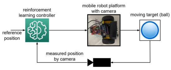
The resulting hardware assembly has a chassis represented by an acrylic plate, having three wheels, two of which are the side ones, the left one being connected to the ADCM so that the assembly can perform rotational (yaw) movements, in order to track a fixed or mobile visual target seen through the webcam [31]. The third wheel is placed in the rear of the chassis; its free motion has solely the role of facilitating the whole assembly yaw motion. On top of the acrylic board and in front of the assembly, the webcam captures images to send back to the PC. The Arduino board was placed in the breadboard, from here making the connection with the ADCM being used, through the H-bridge. The assembly can be observed in Figure 1.

Figure 1. Hardware connection between the engine, motor driver and Arduino Board [31].

Sending commands from the MATLAB environment running on the PC to the ADCM, is handled via Arduino using an USB cable. Arduino sends the commands to the motor driver, which powers the ADCM. The L298n motor driver operates in this project with a single motor. It is powered by a 7.5 V input voltage from a power adapter connected to the outlet that has an output voltage of 7.5 V. Part of this voltage is used to power the ADCM. The ADCM selection was made by connecting the D5 pin to one of the two “Enable” ports of the L298n. Thus, the rotating direction is controlled by the input pins I1 and I2 of the driver, receiving logical voltage level from pins D11 and D12 of Arduino. Depending on the state of these two pins (set or reset), the ADCM spin direction is set. For pin D11 having logical value 1 (5 V) and pin D12 having the value 0 (0 V), the motor will spin clockwise and when D11 has the value 0 and D12 the value 1, the ADCM will spin in counterclockwise direction. In each specific direction, the ADCM’s angular speed is set by a PWM signal generated with Arduino, whose duty cycle value is set in MATLAB and transmitted from the PC. The ADCM is a carbon-brushed motor from Pololu, 6 V, reduction ration 1000:1, with 33 revolutions per minute at no load, drawing a nominal current of 0.1 amps. Due to the high reduction factor, it is ideal for fine low angular speed control.

However, the micro reduction ADCM used is not built for precise position control (as demanded by a video servo tracking system), while a dedicated one is costlier. The ADCM has a variable dead-zone (DZ) around about 0.156 V (per each rotational direction) which is time-varying due to the multiple magnetic and thermal effects that occur after longer time usage. A logical solution is to compensate the DZ, but due to the mentioned phenomena, the DZ thresholds are impossible to compensate exactly. However, an approximate compensation is actually performed, allowing acceptable positioning visual tracking accuracy [31].

In practice, there are certain video tracking platforms involving advanced image processing and features detections techniques, combined with advanced localization techniques of complex motion dynamics, such as unmanned aerial vehicles (UAVs), as done, e.g., in [32]. In work [32] the focus is to ensure tracking reliability under complex practical conditions, including huge scale variation, occlusion and long-term task. Other visual tracking solutions were proposed in [33,34,35]. Such a tracking approach relies on low level controllers which could be designed based on the proposed learning strategies carried out in this work. The main advantage of our platform is its cost efficiency and flexibility, allowing for affordable educational and research activities.

Further on, at the software level, color-based identification of the moving target object (in this project, a blue ball) was performed in MATLAB. The implementation of the object identification process involved several steps. A general position control goal is to track the desired object (blue ball) to keep its position in the image center.

After setting up the desired image capture settings such as resolution ($640\times 360$) and the RGB (red, green and blue) image color type, to be able to process it, the next step is to extract the RGB components. Three 2D matrices are extracted using the commands (in MATLAB code style): r = img (:,:, 1); g = img (:,:, 2); b = img (:,:, 3) where img is the captured image object. To emphasize the tracked object whose blue color is known inside the image, a single 2D matrix is obtained having each pixel intensity level denoted “blueComponent” calculated with (matrix element-wise operation) [31]

$$blueComponent=b –\frac{r}{2}-\frac{g}{2}.$$

(45)

The next step is to set some threshold values in order to identify the regions inside the image that are considered “sufficiently blue”, to include the object to be identified. This is ensured by the bwareafilt function which extracts objects from an image depending on their size or their area. For the detection of unique objects, an analysis of the connected components is performed, in which case each blue region is assigned a unique ID. We ensure that the largest blue object inside the scene is the ball. The image center coordinates being easily calculated as

$$x_c=\frac{n_x}{2}, y_c=\frac{n_y}{2}.$$

(46)

where $n_x, n_y$ are the image width and height, with respect to the top-left corner. Identifying the center of gravity (CoG) of the identified ball object is the next action. The MATLAB function logical first converts numeric values into logical values for the final 2D image. The calculation of the center of gravity of the target object was performed by the regionprops function which measures the properties of a specific region of an image. The function returns the measurements for the property set of each connected component (object) in the binary image. The function can be used for both contiguous or adjacent regions and for discontinuous regions. Regarding these types, we can say about the adjacent regions that they are also called objects, connected components or blobs. The object’s CoG specific coordinates ($o_x$,$o_y$), locates its position within the image. The system’s controlled output is defined as $y=y_c-o_y$. In sample-based measurement in discrete-time, it will denote $y_k$.

To complete the system overview in the proposed design, we denote the PC command sent from the MATLAB environment to the ADCM as the duty cycle factor $u_k\in \left[-1;1\right]$. Regardless of the DZ size, this $u_k$ is sent to the ADCM by adding an offset value for each direction of rotation corresponding to the DZ threshold values. The position reference input $r_k$ sets the desired distance of the object center to the image center. In most applications, $r_k=0$ means that the assembly (the camera in particular) should rotate in order to keep the tracked object in the center. Normally, both $y_k,r_k$ are measured in pixels, leading to a magnitude of hundreds of pixels, depending on the image size. A normalized value of $y_k$ is being used by dividing its pixel value with 1000. Therefore, normalized reference inputs $r_k$ are used as well. The system is capable of consistently processing the frames in native resolution and all the subsequent controller calculations, for a sample period of $T_{\mathit{s}}=0.125 \mathit{s}$. This sample period was established after many statistical evaluations, by timing all the image transfer, visual processing tasks and control law evaluations [31]. Timer objects were used for software implementation convenience, to properly run the recurrent control tasks.

3.2. The Visual Servo Tracking in Model Reference Control Setting

The controlled system is formally described by the discrete-time I/O equation (with $k$ the sample index)

$$y_k=f\left(y_{k-1},\dots ,y_{k-ny},u_{k-1},\dots ,u_{k-nu}\right),$$

(47)

with system control input $u_k\in {\mathsf{\Omega }}_u\subset \Re$ inside the known domain ${\mathsf{\Omega }}_u$, system output $y_k\in {\mathsf{\Omega }}_Y\subset \Re$ in known domain ${\mathsf{\Omega }}_Y$, unknown integer orders $ny,nu\in {\mathbb{Z}}_{+}^{*}$, and unknown dynamic nonlinear continuous differentiable map $f:{\mathsf{\Omega }}_Y\times \dots \times {\mathsf{\Omega }}_Y\times {\mathsf{\Omega }}_u\times \dots \times {\mathsf{\Omega }}_u\to {\mathsf{\Omega }}_Y$. System (47) is assumed to be observable and controllable; these are common data-driven assumptions extracted from working interaction with the system, from technical specifications or from literature survey. Lemma 1 in [36] allows for a virtual state space construct equivalent model of (47) defined as

$$\begin{gathered} x_{k+1}=\mathit{F}\left(x_k,u_k\right), \\ {y}_k=\left[1,0,\dots ,0\right]x_k=x_{k,1}, \end{gathered}$$

(48)

where ${\mathit{x}}_k={[{\mathit{Y}}_{\overline{k,k-\tau }}^T,{\mathit{U}}_{\overline{k-1,k-\tau }}^T]}^T\stackrel{\Delta }{=} {\left[x_{k,1},x_{k,2},\dots x_{k,2\tau +1}\right]}^T\in {\mathsf{\Omega }}_X\subset {\Re }^{2\tau +1}$, more specifically with ${\mathit{Y}}_{\overline{k,k-\tau }}=\left[y_k \dots y_{k-\tau }{]}^T=\right[x_{k,1} \dots x_{k,\tau +1}{]}^T$, ${\mathit{U}}_{\overline{k-1,k-\tau }}=\left[u_{k-1} \dots u_{k-\tau } {]}^T=\right[x_{k,\tau +2} \dots x_{k,2\tau +1}{]}^T$, where $\tau \in {\mathbb{Z}}_{+}^{*}$ has the role of a nonlinear observability index similar to the one in linear systems theory. Here, $\tau$ is defined as the minimal value for which the true state of (48) is recoverable from I/O data samples $u_k, y_k$. When the order of (48) is unknown, so is $\tau .$ In practice, one starts with an initial value and searches for the one which achieves the best control when using the virtual state ${\mathit{x}}_k$ for feedback. Some remarkable features are synthesized in the following observations.

Observation 2. Systems (47) and (48) have the same input and output, hence from I/O perspective their control is the same. The means to achieve control may be different, however the intention is to attempt state feedback control on the virtual system (48) and feed it as input to the true system (47). System (48) is fully state-observable, with measurable states and with partially known dynamics $\mathit{F}(.):{\mathsf{\Omega }}_X\times {\mathsf{\Omega }}_u\to {\mathsf{\Omega }}_X$ where domain ${\mathsf{\Omega }}_X$ is completely known since it is built on known domains ${\mathsf{\Omega }}_u,{\mathsf{\Omega }}_Y$.

Observation 3. Time delays in (47) can also lead to a fully observable description (48) by proper definition of additional states. If present, the (assumed constant) time delays should be known and easily measured from the historical I/O response data.

The visual tracking problem in model reference control intends to find a control law which makes the output $y_k$ in (47) match (or track) the output of a linear output reference model (LORM) best described in its discrete-time state space form as

$$\{\begin{array}{c}{\mathit{x}}_{k+1}^m=\mathit{G}{\mathit{x}}_k^m+\mathit{H}{r}_k,\\ y_k^m=\mathit{L}{\mathit{x}}_k^m,\hfill \end{array}$$

(49)

where ${\mathit{x}}_k^m=\left[x_{k,1}^m,\dots ,x_{k,n_x}^m\right]\in {\mathsf{\Omega }}_{X^m}\subset {\Re }^{n_x}$ is the LORM state, $r_k\in {\mathsf{\Omega }}_R\subset \Re$ is the reference input in known domain ${\mathsf{\Omega }}_R$ and $y_k^m\in {\mathsf{\Omega }}_{Y^m}\subset \Re$ is the LORM output within a known domain. Note that (49) is a state space realization of a more compact linear pulse transfer function (PTF) $M\left(Q\right)$ which relates $y_k^m=M\left(Q\right)r_k$, among all infinite realizations’ triplet $\left(\mathit{G},\mathit{H},\mathit{L}\right)$. Here, $Q$ is the unit time step advance operator ($Q{y}_k^m=y_{k+1}^m$). Selection of $M\left(Q\right)$ is not arbitrary. Under classical model reference control guidelines, it should account for true system dynamics (47) and its bandwidth, and it should include the true system’s time delay and nonminimum-phase dynamic if it is the case.

The ORM control problem is formally expressed as in

$$\begin{gathered} {\mathit{u}}_k^{*}=arg\underset{{\mathit{u}}_k}{min}{V}_{LRMO}^{\infty }\left({\mathit{u}}_k\right), V_{LORM}^{\infty }\left({\mathit{u}}_k\right)={\displaystyle \sum }_{k=0}^{\infty }{\left[y_k\left({\mathit{u}}_k\right)-y_k^m\right]}^2, \\ \mathit{s}.t.\left(48\right),\left(49\right), \end{gathered}$$

(50)

where the explicit dependence of $y_k$ on ${\mathit{u}}_k$ has been captured. The intention is to find an explicit closed-loop control law ${\mathit{u}}_k=\mathit{C}\left({\mathit{s}}_k,r_k\right)$ with ${\mathit{s}}_k$ some regressor state dependent on the control design approach. For example, if ${\mathit{s}}_k={\mathit{x}}_k$, the control renders ${\mathit{u}}_k=C\left(y_k\dots y_{k-\tau },{\mathit{u}}_{k-1}\dots {\mathit{u}}_{k-\tau },r_k\right)$ which is a recurrence equation accommodating many control architectures (PI/PID, etc.). However, other selections of ${\mathit{s}}_k$ are possible, as illustrated in the following sections. Essentially, when driven by the same $r_k$, we should ideally get $y_k=y_k^m$, i.e., the system’s output (also the closed-loop system (CLS) output) equals the ORM output. The class of ORM tracking control problems belong to the “dense rewards” settings, as opposed to the “sparse rewards” case which is found in many AI-related environments, whereas in classical control, the problem is known as a model reference control.

Differently from the model reference adaptive control (MRAC) but nevertheless sharing the same overall goal of output reference tracking, the control solution to (50) should be a stationary, non-adaptive controller. Formulation of the penalty function may impact the resulted control performance significantly. For example, non-quadratic Lyapunov functions serving the role of penalty functions in adaptive control have been proposed in MRAC [37,38]. Based on Observation 1, herein we employ quadratic penalties since we preserve interpretation parallelism with the linear quadratic controller case. A quadratic penalty combined with a linear system renders an infinite-horizon cost that is quadratic convex with respect to the state, which facilitates the existence and uniqueness of a global minimum, but also its analytic derivation. Such desirable properties are expected also with smooth nonlinear systems, to some extent at least.

3.3. Closed-Loop Input-Output Data Collection

The simplest standardized controller, namely the proportional (P)-type one will be used to stabilize the positioning process and to further collect I/O data for finally learning more advanced ORM tracking control. Its transfer function is $H_R\left(\mathit{s}\right)=k_p$, where $k_p$ is the transfer coefficient. As shown in [31], this type of controller is recommended in the case of simple driven processes with a single large time constant, with or without an integral component. In this case, the servo positioning has an integral component. The P controller’s law in discrete-time (with transfer function $H_R\left(Q\right)=k_p$)

$${\mathit{u}}_k=k_p\left({\rho }_k –y_k\right),$$

(51)

is used with $k_p=0.19$ established following experimental tests to give satisfactory tracking performance. Here, ${\rho }_k$ is the reference input to the control system. The tracking scenario implies a sequence of successive piecewise constant reference input values ${\rho }_k$ (each value is kept constant for 10 s) with the amplitude uniformly randomly distributed in $\left[-0.19;0.21\right]$. Additive noise on ${\mathit{u}}_k$ is applied for enhancing exploration (also understood as persistent excitation) with the following settings: the command ${\mathit{u}}_k$ receives an additive noise with uniform random amplitude in $\left[-0.1;0.1\right]$, every three samples.

The ORM continuous-time transfer function is selected as

$$m_{ref}=\frac{{\omega }_n^2}{{\mathit{s}}^2+2\xi {\omega }_n\mathit{s}+{\omega }_n^2},$$

(52)

where ${\omega }_n=1$ sets the response speed and $\xi =0.7$ sets the magnitude overshoot. This transfer function was discretized by using the zero-order hold method with the sampling period $T_{\mathit{s}}=0.125\mathit{s}$, to render:

$$M\left(Q\right)=\frac{0.007367Q+0.006949}{Q^2-1.825Q+0.8395}.$$

(53)

For $M\left(Q\right)$, a state-space controllable canonical form transform is

$$\{\begin{array}{c}{\mathit{x}}_{k+1}^m=\left[\begin{array}{cc}1.8251& -0.8395\\ 1& 0\end{array}\right]{\mathit{x}}_k^m+\left[\begin{array}{c}1\\ 0\end{array}\right]r_k,\\ y_k^m=\left[\begin{array}{cc}0.0074& 0.0069\end{array}\right]{\mathit{x}}_k^m,\hfill \end{array}$$

(54)

which will be used to generate the input-state-output data for the ORM. Meanwhile, a different reference input $r_k$ which excites the ORM was also selected as a sequence of successive piecewise constant values where each value is kept constant for 15 s and the amplitude is uniformly randomly distributed in $\left[-0.19;0.21\right]$. 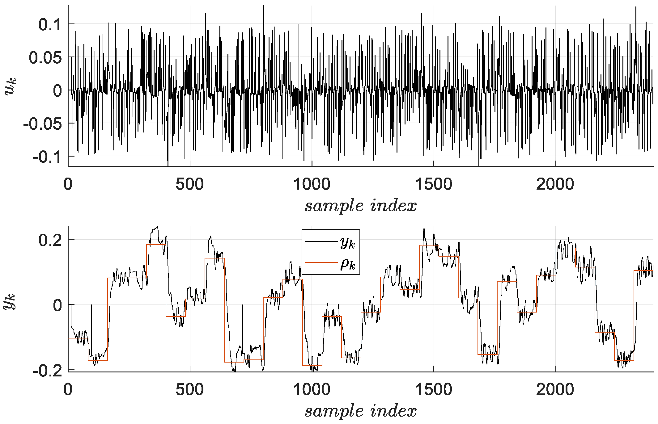The switching periods of the reference inputs ${\rho }_k,r_k$ was not a negligible problem, their values trade-off exploration and lengthy collection time [31]. The I/O data samples contained within the trajectory $\left\{{\mathit{u}}_k, y_k, r_k,{\mathit{x}}_k^m\right\}$ will be subjected to various control design approaches. A number of 2400 samples for 300 s of collection were obtained, as in Figure 2.

Figure 2. I/O data collected from the closed-loop visual servo system.

3.4. The Visual Servo System Identification

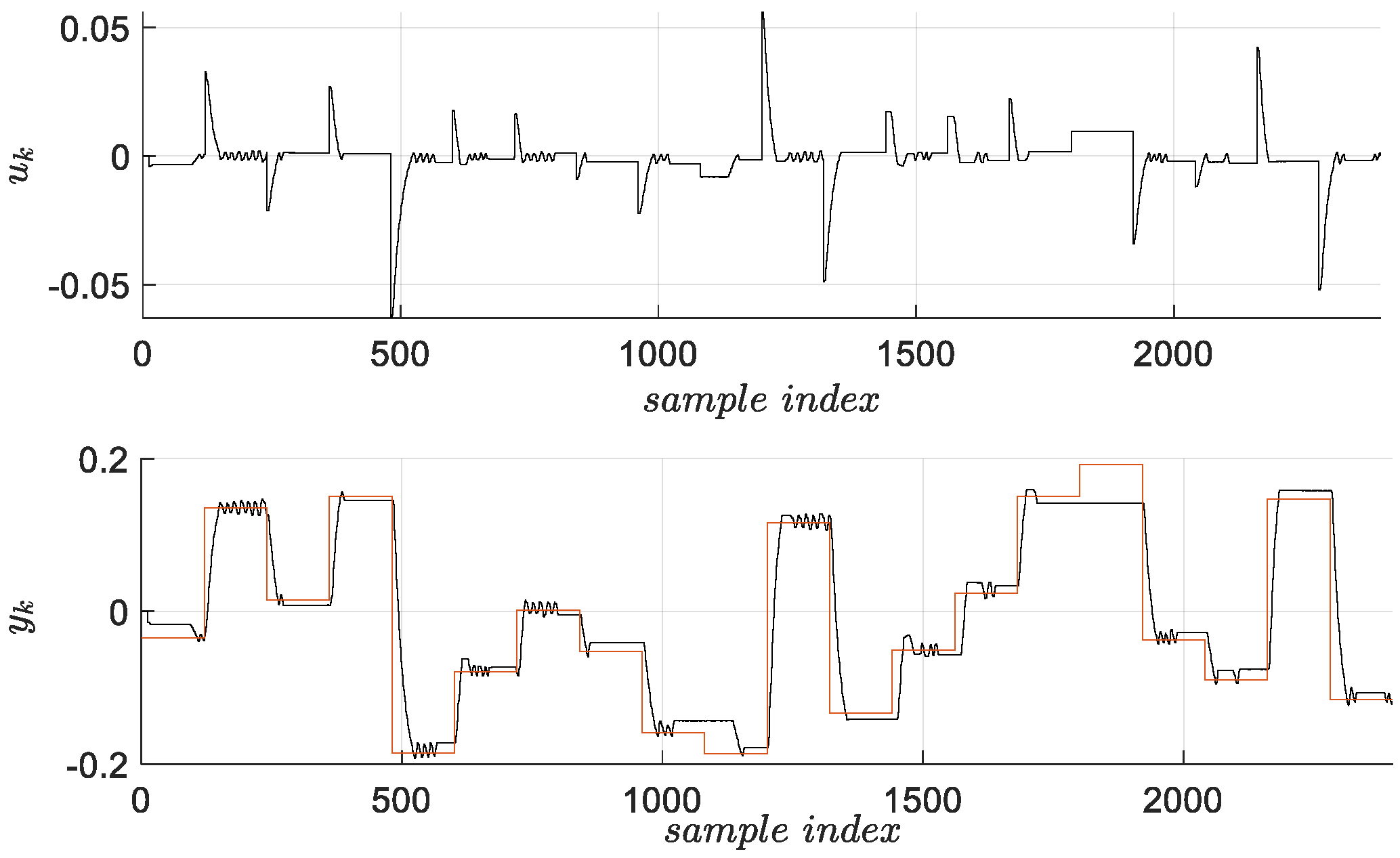
In order to apply a model-based control design dedicated to ORM tracking, a pulse transfer function of the visual servo system must be identified. Since the system has an integral component, the identification is indirectly performed, by firstly identifying the closed-loop pulse transfer function ${\rho }_k\to y_k$, based on closed-loop data from Figure 2 [31]. A set of validation data for the same dynamics is generated, as in Figure 3.

Figure 3. Data used for validating the identified closed-loop visual servo system model (${\rho }_k$-red, $y_k$-black).

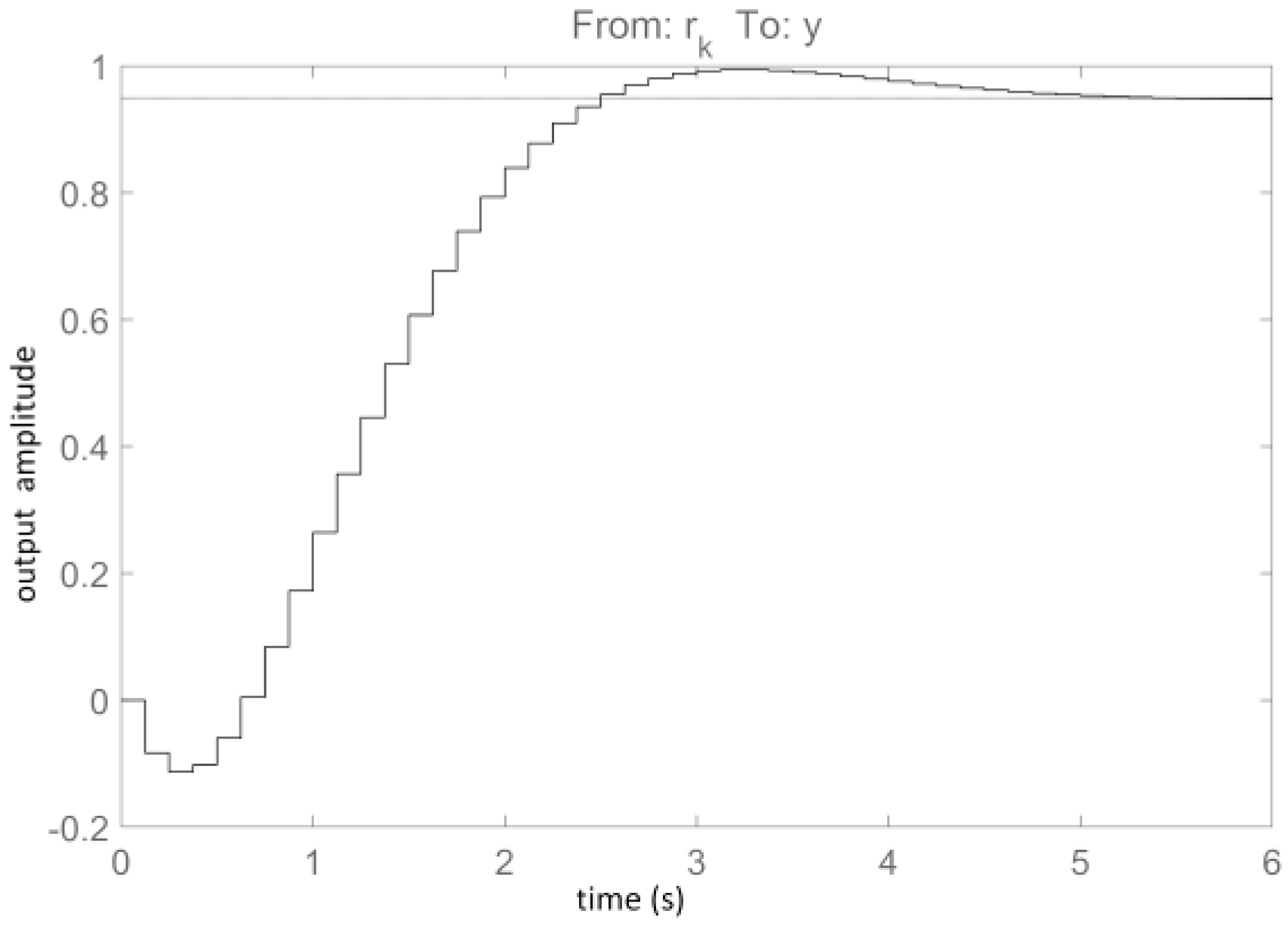
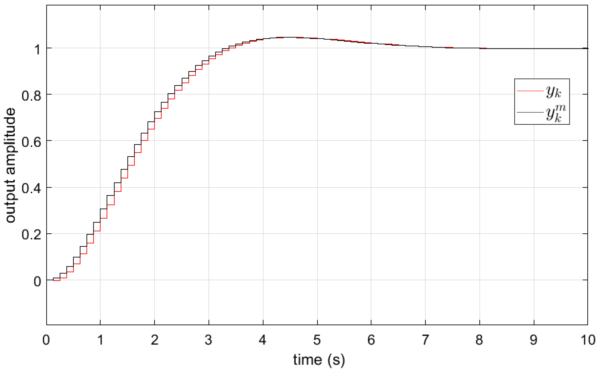
A second-order output-error (OE) recurrent model for the closed-loop visual servo system transfer function is selected, being identified as (and whose step response is shown in Figure 4) [31]

$$M_{CL}\left(Q\right)=\frac{B\left(Q\right)}{F\left(Q\right)}=\frac{-0.08293Q^{-1}+0.1134Q^{-2}}{ 1-1.73Q^{-1}+0.7617Q^{-2}}.$$

(55)

Figure 4. Step response of the OE identified model [31].

The closed-loop transfer function allows for identifying the I/O visual servo system model as [31]

$$H_{PC}\left(Q\right)=\frac{M_{CL}\left(Q\right)}{\left(1-M_{CL}\left(Q\right)\right) H_R\left(Q\right)}=\frac{-0.4365Q^{-1}+0.5966Q^{-2}}{1-1.647Q^{-1}+0.6483Q^{-2}},$$

(56)

whose step response is shown in the Figure 5. Note that the identified $M_{CL}\left(Q\right)$ has a non-minimum-phase character which is not observed in the true system, this non-minimum-phase is a result of the imperfect DZ compensation. Additionally, the model $H_{PC}\left(Q\right)$ appears as a first-order lag with a large time constant, although its true dynamics must contain an integrator. However, the incipient step response phase (first 20 s) overlaps with that of an integral-type system. Finally, the indirectly identified $H_{PC}\left(Q\right)$ can be used for model-based control design.

Figure 5. The step response of $H_{PC}\left(Q\right)$ [31].

3.5. The 2DOF Model-Based Control Design

The 2DOF (also known as RST) control design procedure is next described, for the case with the same imposed dynamics in terms of setpoint tracking and disturbance rejection. Assume that $H_{PC}\left(Q\right)$ can be written in the form

$$H_{PC}\left(Q\right)=\frac{K\left(Q+\beta \right)}{Q^2+{\alpha }_{1}Q+{\alpha }_0}{Q}^{-d}=\frac{B\left(Q\right)}{A\left(Q\right)}{Q}^{-d},$$

(57)

which is validated for the identified model since $\partial \left(B\left(Q\right)\right)=1,\partial \left(A\left(Q\right)\right)=2, d=0$ (the operator $\partial (.)$ measures the polynomial degree) in our case. With the ORM transfer function (53), in the case of the 2DOF controller without stable zero compensation ($H_{PC}\left(Q\right)$ has a non-minimum-phase zero) and with integral component in the controller to ensure zero steady-state tracking error and steady-state disturbance rejection simultaneously, we first define the polynomials as factors for $B\left(Q\right)=B^C\left(Q\right)B^{NC}\left(Q\right)$:

$$B^C\left(Q\right)=1,B^{NC}\left(Q\right)=K\left(Q+\beta \right).$$

(58)

The denominator $A_m\left(Q\right)=Q^2+p_{1}Q+p_0$ from the imposed $M\left(Q\right)$ will actually set the step-response character of the closed-loop system. An artificial, maximal degree polynomial $B_m\left(Q\right)$ is constructed as $B_m\left(Q\right)=\frac{K\left(Q+\beta \right)\left(1+p_1+p_0\right)}{K\left(1+\beta \right)}=\frac{\left(Q+\beta \right)\left(1+p_1+p_0\right)}{1+\beta }$ such that it will simultaneously fulfil a set of conditions set out in [39], namely $\partial \left(B_m\left(Q\right)\right)\le \partial \left(B\left(Q\right)\right)+d$ and $B_m\left(1\right)=A_m\left(1\right).$ After factoring $B_m\left(Q\right)=B^{NC}\left(Q\right){\overline{B}}_m\left(Q\right),$ the polynomial ${\overline{B}}_m\left(Q\right)$ results ${\overline{B}}_m\left(Q\right)=\left(1+p_1+p_0\right)/\left[K\left(1+\beta \right)\right]$.

The polynomials $R\left(Q\right)$, $\mathit{s}\left(Q\right)$ and $T\left(Q\right)$ are imperative in the 2DOF controller design. Firstly, it must be ensured that $\partial R\left(Q\right)=\partial \mathit{s}\left(Q\right)=\partial T\left(Q\right)=n$ [39] where $\partial A\left(Q\right)=\partial A_m\left(Q\right)=n=2$ in our case. Then, $R\left(Q\right)=B^{+}\left(Q\right) \overline{R}\left(Q\right)$ must be monic (leading coefficient is 1) and since $R\left(Q\right)$ must have an integral component, based on $B^C\left(Q\right)=1$, we must further explicit $\overline{R}\left(Q\right)=\left(Q-1\right) \stackrel{=}{R}\left(Q\right)$. Due to the degree condition $n=2$, we must write $\stackrel{=}{R}\left(Q\right)=Q+r_0$. Then, $\mathit{s}\left(Q\right)={\mathit{s}}_2{Q}^2+{\mathit{s}}_{1}Q+{\mathit{s}}_0,$ fulfils the degree condition, while the observer polynomial $A_o\left(Q\right)=Q^2$ is selected to ensure minimal degree fulfilment of the polynomial equation [39]

$$A_o\left(Q\right)A_m\left(Q\right)=A\left(Q\right)\left(Q-1\right)\stackrel{=}{R}\left(Q\right)+B^{NC}\left(Q\right)\mathit{s}\left(Q\right),$$

(59)

equivalent to

$$\begin{gathered} Q^2(Q^2+p_{1}Q+p_0)=\left(Q^2+{\alpha }_{1}Q+{\alpha }_0\right)\left(Q-1\right)\left(Q+r_0\right)+K\left(Q+\beta \right)\left({\mathit{s}}_2{Q}^2+{\mathit{s}}_{1}Q+{\mathit{s}}_0\right)\equiv \\ {Q}^4+p_1{Q}^3+p_0{Q}^2=Q^4+\left(K{\mathit{s}}_2+r_0+{\alpha }_1-1\right)Q^3+\left[K\left({\mathit{s}}_0+\beta {\mathit{s}}_1\right)+{\alpha }_0\left(r_0-1\right)-{\alpha }_1{r}_0\right]Q+K\beta {\mathit{s}}_0-r_0{\alpha }_0. \end{gathered}$$

(60)

The above polynomial equation was solved as a compatible determined system of linear equations in the unknown coefficients of $\stackrel{=}{R}\left(Q\right),\mathit{s}\left(Q\right)$:

$$\{\begin{array}{c}\begin{array}{c}K{\mathit{s}}_2+r_0 +{\alpha }_1- 1 = p_1,\\ K\left({\mathit{s}}_1+\beta {\mathit{s}}_2\right)- r_0+{\alpha }_0+{\alpha }_1\left(r_0-1\right)=p_0,\\ K\left({\mathit{s}}_0+\beta {\mathit{s}}_1\right)+{\alpha }_0\left(r_0-1\right)- {\alpha }_1{r}_0=0,\end{array}\\ K\beta {\mathit{s}}_0 - r_0{\alpha }_0 = 0\end{array}\equiv \left(\begin{array}{cccc}K& 0& 0& 1\\ \beta K& K& 0& {\alpha }_1-1\\ 0& \beta K& K& {\alpha }_0- {\alpha }_1\\ 0& 0& \beta K& -{\alpha }_0\end{array} \right)\left(\begin{array}{c}{\mathit{s}}_2\\ {\mathit{s}}_1\\ {\mathit{s}}_0\\ r_0\end{array}\right)= \left(\begin{array}{c}{p}_1- {\alpha }_{1+1}\\ p_0+ {\alpha }_1- {\alpha }_0\\ {\alpha }_0\\ 0\end{array}\right).$$

(61)

The solution to (61) will produce $R\left(Q\right)$ of the form $R\left(Q\right)=Q^2+r_{1}Q+r_0$. Finally, $T\left(Q\right)={\overline{B}}_m\left(Q\right)A_o\left(Q\right)=t_2{Q}^2$ renders the transfer function description of the 2DOF controller as [31]

$${\mathit{u}}_k=\frac{T\left(Q\right)}{R\left(Q\right)}{\rho }_k-\frac{\mathit{s}\left(Q\right)}{R\left(Q\right)}{y}_k=\frac{t_2{Q}^2}{Q^2+r_{1}Q+r_0}{\rho }_k-\frac{{\mathit{s}}_2{Q}^2+{\mathit{s}}_{1}Q+{\mathit{s}}_0}{Q^2+r_{1}Q+r_0}{y}_k,$$

(62)

which in its recurrent filter form writes as

$${\mathit{u}}_k=-r_1{\mathit{u}}_{k-1}-r_0{\mathit{u}}_{k-2}+t_2{\rho }_k-{\mathit{s}}_2{y}_k-{\mathit{s}}_1{y}_{k-1}-{\mathit{s}}_0{y}_{k-2}.$$

(63)

Using this scheme, we validated the 2DOF controller with the identified system model $H_{PC}\left(Q\right)$ in closed-loop with unit reference input step response, in Figure 6.

Figure 6. Unit reference input step response of the closed-loop with 2DOF controller, vs. the ORM unit step response.

The experimental validation of the designed 2DOF controller used with the true visual servo system is depicted in Figure 7 below, on a test scenario.

Figure 7. The ORM tracking control experiment with 2DOF (blue), VSFRT (red) and MFVI-RL (green) averaged control performance, with 95% confidence regions. $y_k^m$ is in black line in bottom subplot.

3.6. The MFVI-RL Control for ORM Tracking

MFVI-RL requires some Markovian assumptions about the controlled system, hence the controlled extended system will be

$${\mathit{s}}_{k+1}=\mathit{E}\left({\mathit{s}}_k,u_k\right)\iff \left[\begin{array}{c}{\mathit{x}}_{k+1}\\ {\mathit{x}}_{k+1}^m\\ r_{k+1}\end{array}\right]=\mathit{E}\left(\left[\begin{array}{c}{\mathit{x}}_k\\ {\mathit{x}}_k^m\\ r_k\end{array}\right],u_k\right)=\left[\begin{array}{c}\mathit{F}\left({\mathit{x}}_k,u_k\right)\\ \mathit{G}{\mathit{x}}_k^m+\mathit{H}{r}_k\\ t\left(r_k\right)\end{array}\right],$$

(64)

where $\mathit{E}(.)$ is some generic nonlinear map which is partially unknown, ($\mathit{F}(.)$ is partially unknown) over the extended state, and ${\mathit{s}}_k={\left[{\mathit{x}}_k^T,{\left({\mathit{x}}_k^m\right)}^T,r_k\right]}^T$. The domain ${\mathsf{\Omega }}_S$ of ${\mathit{s}}_k$ is known, as the domains ${\mathsf{\Omega }}_X,{\mathsf{\Omega }}_{X^m}, {\mathsf{\Omega }}_R$ are known. In addition, $r_{k+1}=\mathbb{t}\left(r_k\right)$ is the reference input generative model which is user-defined. Many types of practical reference inputs comply with this generative model equation (e.g., piece-wise constant model $r_{k+1}=r_k$).

MFVI-RL is able to learn the ORM tracking control solution for the system (64) without complete knowledge of $\mathit{E}(.)$. The extended states-space system representation (64) can perfectly replace the dynamics (47) in the problem definition (50). Note that $y_k,y_k^m$ in (50) depends on components of ${\mathit{s}}_k$ ($y_k$ is the first component from the vector ${\mathit{x}}_k$ while $y_k^m=\mathit{L}{\mathit{x}}_k^m$). In its off-policy offline version (more popularly known as Q-learning), MFVI-RL starts with a dataset of transition samples (known as tuples or as experiences) of the form $D\mathit{s}=\left\{\left({\mathit{s}}_k^{\left[i\right]},u_k^{\left[i\right]},{\mathit{s}}_{k+1}^{\left[i\right]}\right)\right\}$ for a number of $i=\overline{1,B}$ elements.

MFVI-RL relies on the estimate of a “Q-function” which is an extension of the original cost function $V\left({\mathit{s}}_k\right)=\sum _{i=k}^{\infty }{\gamma }^{i-k}\pi \left({\mathit{s}}_i,u_i\right)$. We notice that $V\left({\mathit{s}}_0\right)=V_{LORM}^{\infty }$ whenever the discount factor $\gamma =1$ and the penalty term is defined, like in $\pi \left({\mathit{s}}_i,u_i\right)={\left(y_i-y_i^m\right)}^2$ which explicitly captures the ORM tracking goal. Using the Bellman equation to which we associate the controller ${\mathit{u}}_k=\mathit{C}\left({\mathit{s}}_k\right)$, the Q-function is defined as $Q^{\mathit{C}}\left({\mathit{s}}_k,u_k\right)=\pi \left({\mathit{s}}_k,u_k\right)+\sum _{i=k+1}^{\infty }{\gamma }^{i-k-1}\pi \left({\mathit{s}}_i,\mathit{C}\left({\mathit{s}}_i\right)\right)=\pi \left({\mathit{s}}_k,u_k\right)+\gamma V^C\left({\mathit{s}}_{k+1}\right)=\pi \left({\mathit{s}}_k,u_k\right)+\gamma Q^{\mathit{C}}\left({\mathit{s}}_{k+1}, \mathit{C} \left({\mathit{s}}_{k+1}\right)\right)$.

To cope with infinitely dense state and control input domains, it is common to parameterize both the Q-function and the controller with (deep) neural networks (NNs). In the following, the MFVI-RL steps with a generic NN approximator for the Q-function (which is expressed as $Q\left({\mathit{s}}_k,u_k,\mathbf{\theta }\right)$ with $\mathbf{\theta }$ being the NN weights) and a linear controller defined by $u_k={\mathit{K}}^T{\mathit{s}}_k=K_0{y}_k+\dots +K_{\tau }{y}_{k-\tau }+K_{\tau +1}{u}_{k-1}+\dots +K_{2\tau +1}{u}_{k-\tau }+K_{2\tau +2}{x}_{k,1}^m+\dots +K_{2\tau +n_x+1} x_{k,n_x}^m+K_{2\tau +n_x+2} r_k$ where $\mathit{K}\in {\Re }^{2\tau +n_x+2}$, are presented in Algorithm 1.

Algorithm 1. The MFVI-RL Algorithm 1 for ORM tracking

Choose a reference model with dynamic $M\left(Q\right)$, under the rules and in terms of specifications which are representative for model reference control. Build a state space realization (49) from $M\left(Q\right)$. Run data collection experiments on system (47) to obtain a dataset of I/O samples $\left\{u_k, y_k\right\}$. In the same time-frame or in a simulated process afterwards, generate $\{r_k,{\mathit{x}}_k^m,y_k^m\}$ using a prescribed generative reference input model $r_{k+1}=\mathbb{t}\left(r_k\right)$ and the state-space (49). Make sure the domains ${\mathsf{\Omega }}_Y$ and ${\mathsf{\Omega }}_{Y^m}$ are correlated in amplitude. The collection of both $\left\{u_k, y_k\right\}$ and $\{r_k,{\mathit{x}}_k^m,y_k^m\}$ must be sufficiently exploratory i.e., the variables should cover all combinations of their values inside their respective domains. This is usually achieved for long enough trajectories. However, good coverage of the state-action space in a shorter time is achievable in various ways: straightforward procedures include adding noise and avoiding already visited combinations by recording the tracks. Select the observability index $\tau$. Data-driven construct the virtual trajectory $\left\{u_k, y_k,{\mathit{x}}_k\right\}$ which defines the virtual state-space system (49). Couple this trajectory with $\{r_k,{\mathit{x}}_k^m,y_k^m\}$ to construct transition samples $\left({\mathit{s}}_k^{\left[i\right]},u_k^{\left[i\right]},{\mathit{s}}_{k+1}^{\left[i\right]}\right),$ $i=\overline{1,B}$ from (64). Select an initial parameterization for the NN modeling the Q-function, let this be denoted as $Q\left({\mathit{s}}_k,u_k,{\mathbf{\theta }}^0\right)$ where ${\mathbf{\theta }}^j$ lumps all the NN tunable weights at iteration $j$. Select ${\mathit{K}}^0$ as the initial controller parameter, it need not be stabilizing for MFVI-RL algorithm (e.g., random initial value is feasible). At current iteration $j$, prepare the Q-function NN input patterns as $in\mathit{s}=\left\{{[{\mathit{s}}_k^{{\left[i\right]}^T}, u_k^{\left[i\right]}]}^T\right\}$ and the target output patterns as $out\mathit{s}=\left\{\pi \left({\mathit{s}}_k^{\left[i\right]},u_k^{\left[i\right]}\right)+Q\left({\mathit{s}}_{k+1}^{\left[i\right]}, {\mathit{K}}^{j-1^T}{\mathit{s}}_{k+1}^{{\left[i\right]}^T}, {\mathbf{\theta }}^{j-1}\right)\right\}$, for all $i=\overline{1,B}$. Train the NN using the I/O patterns, based on architecture-dependent training settings. It is equivalent to solving ${\mathbf{\theta }}^j=arg\underset{\mathbf{\theta }}{min}\frac{1}{B}\sum _{i=1}^B{\left( Q\left({\mathit{s}}_k^{\left[i\right]}, {\mathit{u}}_k^{\left[i\right]}, \mathbf{\theta }\right) - \pi \left({\mathit{s}}_k^{\left[i\right]}, u_k^{\left[i\right]}\right) - Q\left({\mathit{s}}_{k+1}^{\left[i\right]}, {\mathit{K}}^{j-1^T}{\mathit{s}}_{k+1}^{\left[i\right]}, {\mathbf{\theta }}^{j-1}\right)\right)}^2$ which is the well-known MSSE cost. For each ${\mathit{s}}_k^{\left[i\right]},i=\overline{1,B}$ in the dataset, find $u_k^{{\left[i\right]}^{*}}=arg\underset{u}{min}Q\left({\mathit{s}}_k^{\left[i\right]},u,{\theta }^j\right)$. For a bounded infinite domain e.g., ${\mathsf{\Omega }}_u=\left[-1;1\right]$, this minimization will be approximately done by enumerating a finite set of equidistant values for $u$ e.g., $\left\{-1,-0.9,\dots ,0.9,1\right\}$. Although apparently exhaustive and not as accurate as a gradient based search scheme, this minimization can be efficiently implemented even for multivariable systems where the dimension of ${\mathsf{\Omega }}_u$ is acceptable (up to three). Build the overdetermined system of linear equations $$\left[\begin{array}{c}{\left({\mathit{s}}_k^{\left[1\right]}\right)}^T\\ \dots \\ {\left({\mathit{s}}_k^{\left[B\right]}\right)}^T\end{array}\right]{\mathit{K}}^j=\left[\begin{array}{c}{u}_k^{{\left[1\right]}^{*}}\\ \dots \\ u_k^{{\left[B\right]}^{*}}\end{array}\right]\iff {\mathit{\Xi }}_{\mathit{1}}{\mathit{K}}^j={\mathit{\Xi }}_{\mathit{2}},$$ (65) and solve it by ordinary linear least-squares as ${\mathit{K}}^j=pinv\left({\mathit{\Xi }}_{\mathit{1}}\right){\mathit{\Xi }}_{\mathit{2}}$ where $pinv\left({\mathit{\Xi }}_{\mathit{1}}\right)={\left({{\mathit{\Xi }}_{\mathit{1}}}^T{\mathit{\Xi }}_{\mathit{1}}\right)}^{-1}{{\mathit{\Xi }}_{\mathit{1}}}^T$. Another possible gradient-based search solution for finding ${\mathit{K}}^j$ is to train the cascaded network $Q\left({\mathit{s}}_k^{\left[i\right]},{\mathit{K}}^T{\mathit{s}}_k^{\left[i\right]},{\mathbf{\theta }}^j\right)$ w.r.t. $\mathit{K}$, over all inputs ${\mathit{s}}_k^{\left[i\right]},i=\overline{1,B}$, with the target values set to zero. If the number of maximal MFVI-RL algorithm iterations was reached, or there is no improvement in the control parameter ($\Vert {\mathit{K}}^j-{\mathit{K}}^{j-1}\Vert <thre\mathit{s}hold$), exit the algorithm; otherwise increment $j$ and go to step 5.

For the MFVI-RL practical implementation of learning visual servo tracking, the Q-function is a deep neural network of feedforward type, with two hidden layers having 100 and 50 rectified linear unit (ReLU) activation function, respectively. A single neuron in the output with linear activation predicts the Q-value of a state-action input. Training settings include: 90%–10% training-validation data splitting with random shuffling; early stopping after 10 consecutive increases of the MSSE cost on the validation data; and maximum 500 epochs with a scaled conjugated gradient descent backprop algorithm. The entire training data is used as one batch in each epoch, therefore the “replay buffer” consists of all the transition samples in the experience replay mechanism. This can be considered a deep reinforcement learning approach belonging to the supervised machine learning field.

Starting with the I/O data collection from the closed-loop system under the P-type controller and with the ORM input-state-output data collected offline, the trajectory $\left\{u_k, y_k, r_k,{\mathit{x}}_k^m\right\}$ has 2400 samples out of which only 2369 obey the piecewise-constant generative reference input model $r_{k+1}=r_k$. A total number of 100 iterations lead to the MFVI-RL controller matrix $\mathit{K}={\left[-0.6337,0.3008,-0.1373,-0.0838,-0.0527,-0.0007,0.0041,0.3094\right]}^T$ for the controller modeled as $u_k={\mathit{K}}^T{\mathit{s}}_k$, shown performing in Figure 7. We stress that the linear controller structure complies very well with the 2DOF controller structure (and with the subsequent VSFRT controller structure), in an attempt to investigate and check the best achievable framework-dependent control performance.

3.7. The VSFRT Learning Control Design for ORM Tracking

The VSFRT feedback control concept is briefly detailed in this section. Since it relies on state information for feedback, it uses again a state-space model, this time it is the model (48), together with a different rationale for computing offline the virtual reference input. It generalizes over the classical nonlinear virtual reference feedback tuning (VRFT) concept [40,41,42,43,44,45,46,47] in the sense that the control law is not explicitly depending on the output feedback error as in $u_k=\mathit{C}\left(e_k=r_k-y_k\right)$ but rather in the form $u_k=\mathit{C}\left({\mathit{x}}_k, r_k\right),$ or, more generally, depending on the lumped regressor ${\mathit{s}}_k={\left[x_k^T, r_k\right]}^T$ hence resulting in the law $u_k=\mathit{C}\left({\mathit{s}}_k\right).$ Starting from a dataset of I/O samples $\left\{u_k, y_k\right\}$ collected from the system (47), VSFRT computes the virtual trajectory $\left\{u_k, y_k,{\mathit{x}}_k\right\}$ of (48) first. The virtual reference is afterwards computed as ${\tilde{r}}_k=M^{-1}\left(Q\right)y_k$. From this, the virtual lumped regressor builds the dataset of states as $\left\{{\mathit{s}}_k={\left[x_k^T, {\tilde{r}}_k\right]}^T\right\},k=\overline{1,B}$. The VSRFT principle solves (50) indirectly by solving a controller identification problem posed as [48]

$${\mathbf{\vartheta }}^{*}=arg\underset{\mathbf{\vartheta }}{min}{V}_{VR}^N\left(\mathbf{\vartheta }\right), V_{VR}^N\left(\mathbf{\vartheta }\right)=\frac{1}{B}{\displaystyle \sum }_{k=1}^B{\left(u_k-\mathit{C}\left({\mathit{s}}_k,\mathbf{\vartheta }\right)\right)}^2,$$

(66)

which specifies that the controller fed with ${\mathit{s}}_k$ and parameterized by $\mathbf{\vartheta }$ should output $u_k$ obtained in the first place in the collection phase. A remarkable observation is that ${\mathit{s}}_k$ in VSFRT does not contain the ORM state ${\mathit{x}}_k^m$ as in the MFVI-RL case, since it is viewed as an unnecessary redundancy [24]. Hence, the ORM state-space model is useless, except for its I/O model $M\left(Q\right)$. VSFRT does not require the Markovian assumption about the system state-space model, hence it does not require a reference input generative model because the VRFT principle is different about getting $r_k$. The VSFRT steps are next described in Algorithm 2 for the case of a linear control $u_k={\mathit{K}}^T{\mathit{s}}_k=K_0{y}_k+\dots +K_{\tau }{y}_{k-\tau }+K_{\tau +1}{u}_{k-1}+\dots +K_{2\tau +1}{u}_{k-\tau }+K_{2\tau +2}{r}_k$ where $\mathit{K}\in {\Re }^{2\tau +2}$ (notice the resemblance with MFVI-RL control, except for the ORM states). In the linear controller case, $\mathbf{\vartheta }=\mathit{K}$.

Algorithm 2. The VSFRT Algorithm 2 for ORM tracking

Choose a reference model dynamic $M\left(Q\right)$ under the rules and in terms of specifications which are representative for model reference control. Run data collection experiments on system (47) to obtain a dataset of I/O samples $\left\{u_k, y_k\right\}$. Here, $u_k$ should be persistently exciting to make $y_k$ capture all of the system’s dynamics. This is a sort of exploration condition, as in MFVI-RL. The excitation condition is usually ensured by (additive) exploratory noise, whether in an open- or in closed-loop. Select the observability index $\tau$. Data-driven build the virtual trajectory $\left\{u_k, y_k,x_k\right\}$ which defines the virtual state-space system (48). Compute the virtual reference input as ${\tilde{r}}_k=M^{-1}\left(Q\right)y_k$. Here, a series of aspects are of interest. $M\left(Q\right)$ commonly has a low-pass behavior, making $M^{-1}\left(Q\right)$ as a high-pass filter. If $y_k$ is noisy, low-pass prefiltering is strongly advised, which could be done, for instance, as a zero-phase filtering. This filtering is not the same as the classical VRFT pre-filter $L\left(Q\right)$ as it is not applied on the entire regressor vector ${\mathit{s}}_k$ but only on $y_k$. Further, even if $M^{-1}\left(Q\right)$ is non-causal, it can be implemented offline. Build the regressor vector $\left\{{\mathit{s}}_k={\left[{\mathit{x}}_k^T, {\tilde{r}}_k\right]}^T\right\},k=\overline{1,B}$. Form the overdetermined system of linear equations $$\left[\begin{array}{c}{\mathit{s}}_1^T\\ \dots \\ {\mathit{s}}_B^T\end{array}\right]K=\left[\begin{array}{c}{u}_1\\ \dots \\ u_B\end{array}\right]\iff {\Xi }_{\mathbf{1}}\mathit{K}={\Xi }_{\mathbf{2}},$$ (67) and solve it by ordinary linear least-squares as $\mathit{K}=pinv\left({\Xi }_{\mathbf{1}}\right){\Xi }_{\mathbf{2}}$ where $pinv\left({\Xi }_{\mathbf{1}}\right)={\left({{\Xi }_{\mathbf{1}}}^T{\Xi }_{\mathbf{1}}\right)}^{-1}{{\Xi }_{\mathbf{1}}}^T$. This, in fact, solves the controller identification (66) over the controller parameter $\mathit{K}$.

Commonly, nonlinear controllers modeled as NNs have also been employed in many settings [24,48,49,50,51,52,53,54]. Most of these deal with tracking applications extensively [55,56,57,58,59,60,61,62]. In the case of mildly nonlinear systems, linear state-feedback controllers, such as the proposed one, have proven functional. In fact, using the input patterns $\left\{{\mathit{s}}_k\right\}$ and the output patterns $\left\{u_k\right\}$, one can train any approximator for the controller using appropriate methods by minimizing the cost function (66), which is the popular MSSE cost. Several intercoupled aspects of how can VSFRT serve for transfer learning to the MFVI-RL controller have been thoroughly investigated in [24], where other aspects, such as using principal component analysis and autoencoders for dimensionality reduction of the state, have been tested as well. Depending on the VSFRT NN controller complexity, it can be framed within the deep learning type of applications.

For our practical implementation on the visual servo tracking, the same dataset of I/O data was used for VSFRT control design; namely, there were 2400 samples of trajectory $\left\{u_k, y_k,{\mathit{x}}_k\right\}$. There is no need for a specific generative reference input model, hence all samples were used. Before computing the virtual reference ${\tilde{r}}_k=M^{-1}\left(Q\right)y_k$, the output was prefiltered through the low-pass filter $QM\left(Q\right)$. The reason is that there exists some high-frequency content in $y_k$ due to the imperfect DZ compensation in the collection experiment with the P-type controller. Different from the classical VRFT setting, the role of the prefilter here is not to make the controller identification cost function match the ORM tracking cost function, but to merely minimize the DZ’s negative influence. Solving (66) with (67) renders $\mathit{K}={\left[-0.3469,-0.1222, 0.1001, 0.0488, 0.0060, 0.3565\right]}^T$ and the resulted VSFRT controller is $u_k={\mathit{K}}^T{\mathit{s}}_k$, performing in Figure 7.

3.8. Testing the Controllers and Measuring the Resulted Tracking Control Performance

For a fair evaluation of the ORM tracking control, the index

$$fi{t}_{\mathit{s}core}[\%]=100\left(1-{\displaystyle \sum }_{i=1}^N{\left(y^k-y_k^m\right)}^2/\left({\displaystyle \sum }_{i=1}^N{\left(y^k-{\overline{y}}_k\right)}^2\right)\right),$$

(68)

was measured, where the mean value is defined ${\overline{y}}_k=1/N\sum _{i=1}^N{y}_k$ for $N=950$ samples. This fit score metric is more practical and correlates well with the cost $V_{LORM}^{\infty }$ in (50). It also represents the percentage expression of the $R^2$ Pearson coefficient of determination used in statistics. The ORM tracking performance for the visual servo system is shown in Figure 7, in terms of mean response and 95% confidence intervals obtained after five runs with each of the 2DOF, MFVI-RL and VSFRT controllers. The actual values of $fi{t}_{\mathit{s}core}$ are rendered in Table 1 below.

Table 1. 2DOF, VSFRT and MFVI-RL tracking performance score when learning uses closed-loop IO data, measured on $fi{t}_{\mathit{s}core}$ [%] [31].

Trial	2DOF	VSFRT	MFVI-RL
1	75.4897%	18.8667%	80.8252%
2	62.1113%	25.3567%	81.9418%
3	73.7258%	49.2332%	78.1441%
4	70.1448%	39.4324%	72.6856%
5	69.4888%	54.4153%	73.2465%
Average	70.1921%	37.4609%	77.3686%
Std	5.1563%	15.1837%	4.2540%

From a testing viewpoint, we do not move the blue ball target manually since this behavior is hardly reproducible. Instead, we change the reference setpoint distance of the image center with respect to the detected blue ball as a sequence of piecewise constant steps. This piecewise constant variation of the reference is then filtered through the linear ORM. This ORM’s output should be tracked accordingly with all tested controllers (An illustration of the test scenario with the MFVI-RL controller is to be found in the movie that can be accessed and viewed at the following address https://drive.google.com/file/d/1VI8mbi7GOyaOE4ceIxJyaEPvRVBqTQPP/view?usp=sharing (accessed on 7 November 2021)).

A linear controller parameterization was used in this case study, to verify and discriminate the control capability of MFVI-RL and VSFRT, compared to the model-based 2DOF controller. As seen from the results recorded in Table 1, the MFVI-RL controller achieves the best statistical result, even better than the 2DOF model-based controller, which supports the conclusion that model-free design can in fact surpass the model-based design which relies on approximate identified system models. The inferiority of VSFRT with respect to both the baseline 2DOF controller and MFVI-RL controller, observed in Table 1, indicates that the I/O data exploration issues is the main responsible factor. This conclusion is supported by the fact that VSFRT has been shown to be superior to MVFI-RL when applied to other systems, such as aerodynamic or robotic ones [24]. In fact, VSFRT was able to learn better control with fewer transition samples and with less exploration. This observation confirms that the exploration issue in data-driven control is still an open problem and efforts are needed to define exploration quality indexes. These indexes must be accounted for and balance the overall responses to the big questions of data-driven control, such as what is the tradeoff between the controller complexity and parameterization vs. the control goal vs. the optimal data volume and exploration quality?

On the application level, all three compared controllers are limited in the achievable linear ORM tracking performance. The reason lies with the visual servo system actuation quality from the ADCM: it has a time-varying dead zone whose thresholds in each rotation direction change with longer runs, owing to electromagnetic effects. A perfect compensation is therefore impossible to achieve without an adaptive mechanism. The used ADCM is certainly not suitable for quality positioning systems. Under these adversarial settings, the learned control for the visual servo system ORM tracking is deemed satisfactory and it achieved the desired quality level. With better actuators, the tracking performance is certainly expected to increase. In conclusion, such video servo systems are widely usable in real world applications, such as surveillance cameras, motion tracking, etc.

4. Conclusions

Learning controllers from I/O data based on the new virtual state representation was validated in a data-driven style using MFVI-RL and VSFRT frameworks. This validation is important since, on one hand, it makes a strong connection between modern control concepts and classical control concepts such as ORM tracking, two-degrees-of-freedom control and classical control performance indices. On the other hand, it uses machine learning methods and tools to achieve the control goal, therefore bridging the gap between control systems and artificial intelligence. The generalizability of these techniques is straightforward extendable to more, nonlinear, multivariable systems. Validation on more systems like the visual servo will confirm the viability of the proposed frameworks and open the road to more systematic investigations. It will also lead to automatic control design tools with powerful generalization capability, belonging to the next generation of intelligent and autonomous control systems.