A Scalable Control Strategy for CHB Converters in Photovoltaic Applications

Abstract

Renewable energy sources are becoming more relevant in recent decades in power generation, leading to investment in developing efficient systems. Specifically, in photovoltaic energy, modular converters are attracting interest since their characteristics enable them to work at high voltage and optimize the generated energy. However, the control strategies found the literature limit the scalability potential of modular converters. The main aim of this paper is to propose a scalable control strategy for a grid-tied CHB (Cascaded H-Bridge) converter for large-scale photovoltaic power plants. The control proposed is able to take full advantage of converter scalability and modularity, being based on the parameters needed for bipolar sinusoidal PWM (Pulse Width Modulation), and thus reducing the calculus required and simplifying its implementation. Power imbalances are overcome including the zero-sequence vector injection to allow power exchange between phases. Furthermore, the parameter used for power factor control has been discretized and discretization time analysis shows that the control strategy is stable and does not require a high-speed communication channel. For validation purposes, simulations are conducted on a downsized 12 H-bridge model.

1. Introduction

In the last decade, renewable sources of energy have become more competitive due to the major reduction in costs of wind and solar energies [1]. Moreover, battery-based energy storage systems have also seen how their costs have dropped dramatically [2]. As a consequence, a large proportion of the electric energy generated throughout the world is expected to come from a renewable source of energy by the year 2050 [3], also achieving a significant reduction in pollution.

The increase in the number of renewable source power plants which are connected to the grid on a mass scale is going to entail a challenge for the grid as a whole. For low power applications, micro inverters have been developed as shown in [4,5]. However, for utility scale photovoltaic plants, converters have to face other challenges. From the technological perspective, the high stress under which the semiconductor devices will have to operate is the main limitation, especially high voltage stress, due to the fact that, depending on the power of the power station, connection line voltage may be higher than 66 kV [6].

As a result, multilevel converters have become common architectures in this area. In [7], an NPC (Neutral Point Clamped) converter handles 40 MVA connected to 3.3 kV and 4.16 kV grids, with the trend showing that photovoltaic plant capacity is increasing up to several MW and will continue to do so in the future. Nonetheless, as a consequence of the increasing voltage and power at which switching devices have to operate, the widely used two-level inverter and NPC type converters result in inefficient or unviable solutions when it comes to applications such as large photovoltaic plants [8].

Thus, topologies with modular capacity, such as the CHB topology [9,10,11], have gained attention lately because they allow devices to operate with lower voltage, obtaining a final output that may be several times higher. Indeed, the modular nature of the CHB topology is at the root of its potential scalability, providing a more efficient maximum power point tracking (MPPT) feature than their two-level counterparts [12,13].

Regarding control strategies for CHB converters, it is possible to find methods based on direct power control [14], although voltage-oriented control (VOC) is the most commonly used [15,16,17]. The control scheme for grid-tied CHB inverters based on VOC usually consists of a voltage loop that controls the equivalent DC voltage, measuring the capacitor voltage of each H-bridge. Additionally, dq current control loops [18], imbalance control and inter-module H-bridge balancing control generate the voltage references for Phase Shifted Pulse Width Modulation (PS-PWM) [19,20]. The main drawback of this compensation method is that the number of I/O signals and ADC (Analog to Digital Converter) channels that are required for control is limited by the controller (DSP or FPGA), greatly reducing scalability of the CHB topology. Moreover, the computational load needed to perform these types of control strategy is rather high.

There have been numerous attempts to ensure a distributed control technique for CHB inverters with a view to solving the scalability problem. Authors in [21,22] propose distributed control strategies that rely on complex communication networks involving EtherCAT (Beckhoff Automation) or optical fiber. In addition, as the references sent to each H-bridge are different, they may overload the communication channel in large-scale power plants. In [23], a distributed control strategy is proposed, but there is a centralized modular converter integrated in the system that regulates the currents injected into the grid, which means limiting scalability.

Consequently, to take advantage of the modular nature of the CHB topology and expand its scalability feature without using a high-speed communication protocol, this paper proposes a novel scalable control strategy for large photovoltaic power plants. The novelty of the control technique is using the sinusoidal modulation instead of the vector modulation employed in VOC-based strategies. The sinusoidal modulation enables the use of specific control variables to regulate different aspects of the converter independently. On the one hand, a controller that takes place in each cell measures a local variable to regulate the power delivered by each cell. On the other hand, a global controller measures the global variables to control the power factor and compensate imbalances. The global controller includes zero-sequence vector injection to prevent distortions in the currents injected when there are imbalances in the power generated by each phase [24].

The paper is structured as follows: in Section 2, the system as a whole is described, while in Section 3, the control strategy is analyzed. Subsequently, simulation results are shown in Section 4 and finally the conclusions are provided in Section 5.

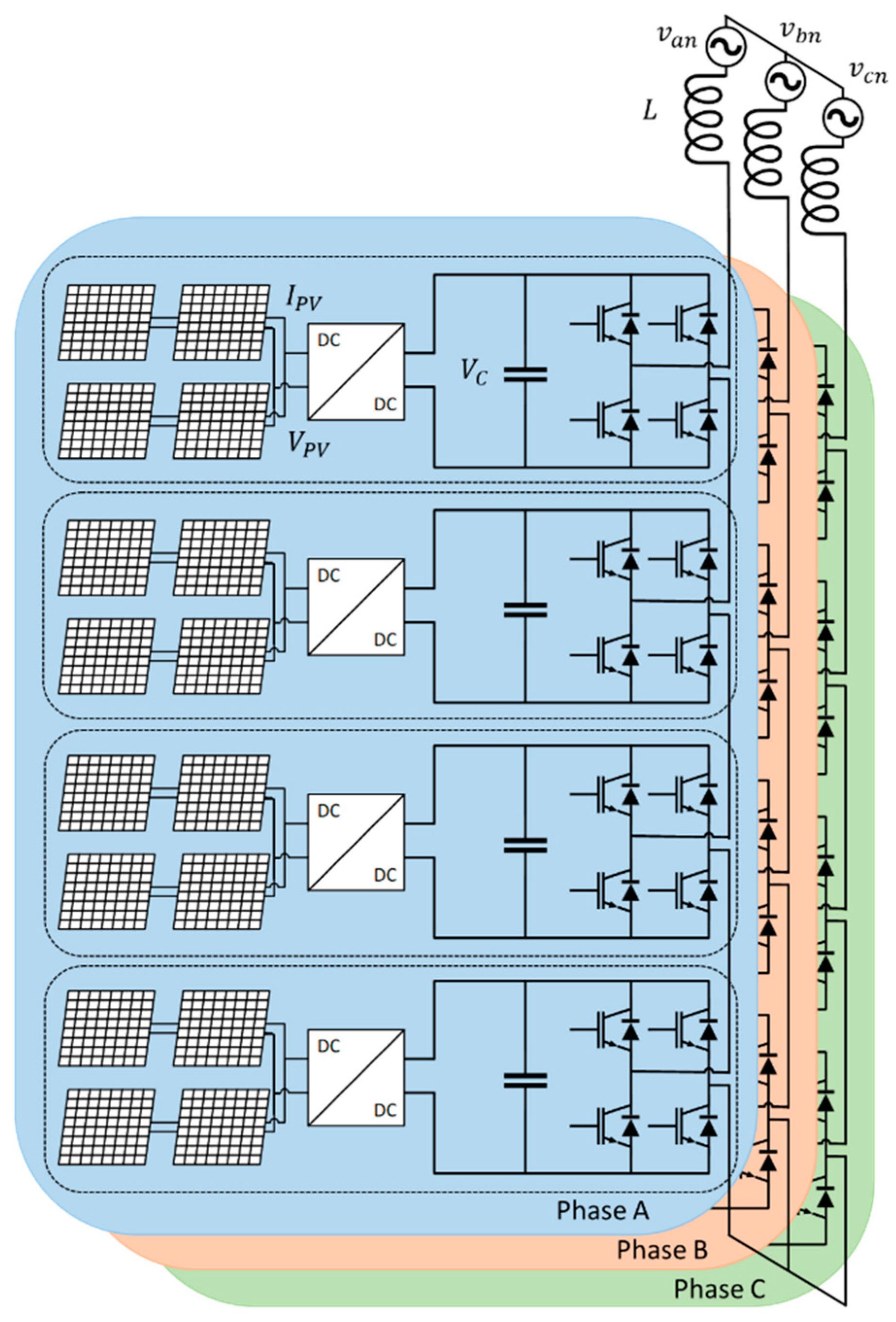
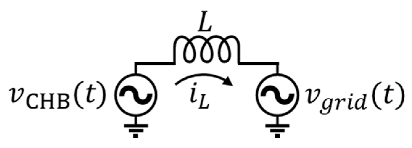
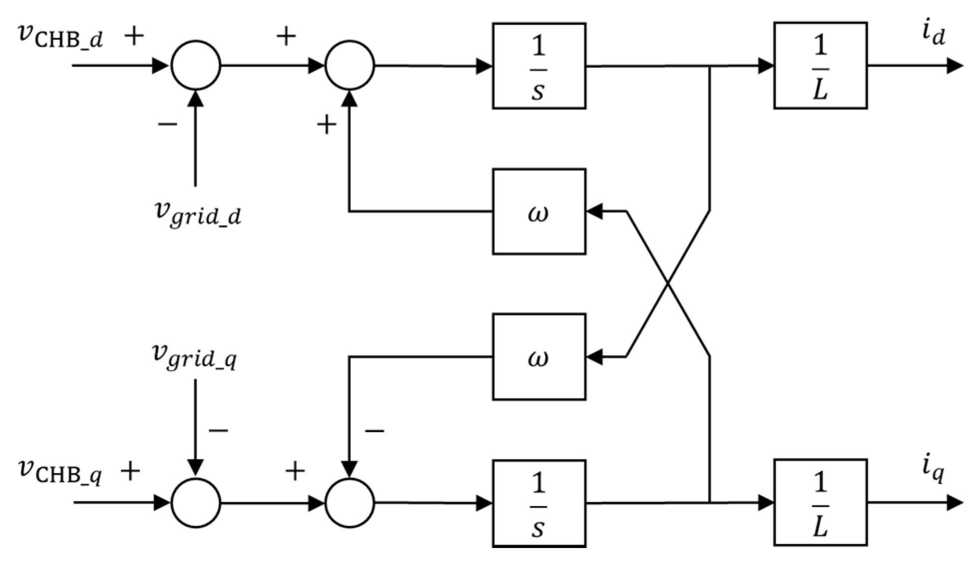
2. System Description

The control strategy proposed is applied to a CHB grid-tied inverter in a photovoltaic plant, as shown in Figure 1. The CHB inverter consists of 12 H-bridges grouped into four cells per phase. In addition, in each cell, there are solar panels and a DC/DC converter.

The H-bridge of each cell is connected to the photovoltaic panels through isolated unidirectional DC/DC converters whose main function is to perform the MPPT algorithm based on voltage and current measurements of the photovoltaic panels (V_PV and I_PV, respectively). As a high voltage DC bus can cause damage to the panels due to isolation issues and some countries have limitations and regulations governing this [25], the DC/DC converters must provide galvanic isolation to prevent a high voltage DC bus from being created in the side of the solar panels. The behavior of the group formed by the solar panels and the DC/DC converter can be modeled as a current source according to [26], as it is separate from the control proposed.

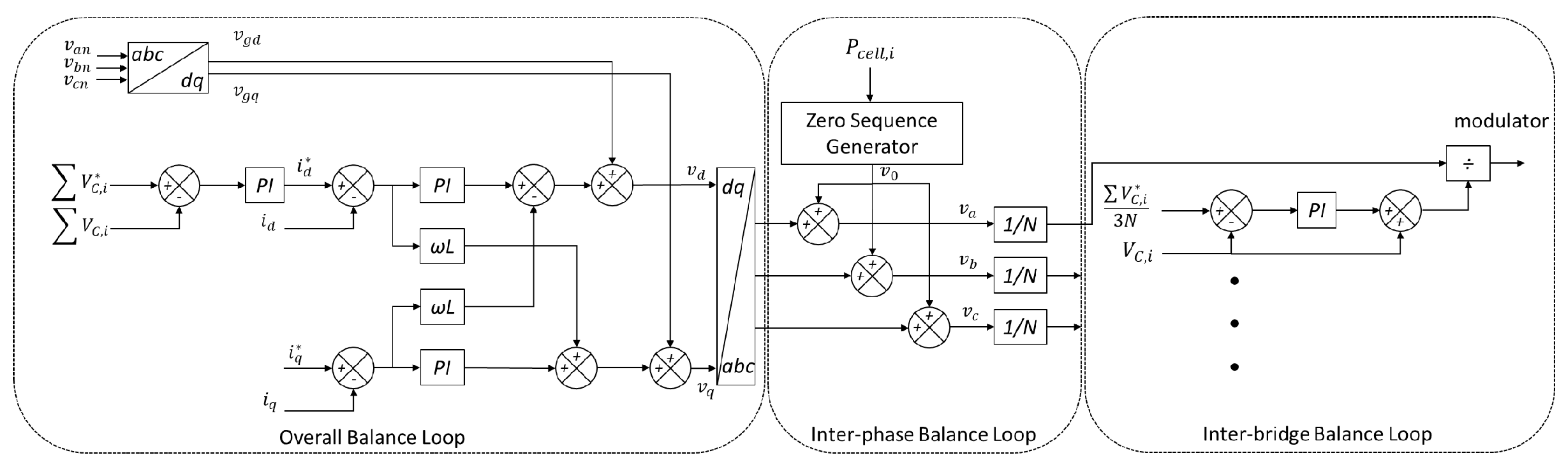
3. Scalable Control Strategy

In the last few years, VOC control has been widely used to control CHB converters and forms the basis of other control strategies [21,22,23,24]. Figure 2 shows a VOC control scheme, which includes the zero-sequence vector injection, applied to an N cell per phase CHB grid-tied converter. There are three different sections in the control scheme: the overall balance loop, the inter-phase balance loop and the inter-bridge balance loop. The first one regulates the equivalent DC voltage bus, which is the sum of the voltage of each capacitor, generating the direct current reference and performing the current control loops. The quadrature current reference is set according to the reactive power requested by the grid controller [27]. The central section generates the zero-sequence vector that modifies the voltage references to compensate inter-phase imbalances and, in the last one, 3N PI controllers regulate the capacitor voltage of each cell.

In the strategies based on schemes similar to the one shown in Figure 2, the scalability of CHB converters is limited because they require too many I/O signals as the number of cells grows, or they rely on complex communication protocols.

The scalable control strategy proposed focuses on the parameters included in bipolar sinusoidal PWM (B-SPWM) modulation [28] of the H-bridges. These parameters are the electric angle (ωt), the modulation index (m) and the phase delay (δ). The electric angle guarantees synchronization with the grid, while the modulation index regulates the active power delivered by each cell to the grid, which is mostly equal to the power generated by the photovoltaic panels. The phase delay, which is the same for all cells, controls the power factor of the whole system.

As shown in Figure 3, there are two different types of controllers in the scalable control proposed: one for each cell and another for global system control. CHB cell control, which is implemented in each cell, regulates the active power delivered by each cell by adjusting the modulation index to control capacitor voltage. This controller is equivalent to the loop that regulates the global DC voltage bus in the overall balance loop and the inter-bridge balance loop in VOC control. The global system control regulates the system power factor by modifying the phase delay and includes the zero-sequence vector injection in order to compensate for any power imbalance between phases. Hence, it plays the same role as the current control loops of the overall balance control and the inter-phase balance loop of the VOC control method. The global system control is outside the CHB cells, and so the control strategy proposed needs a communication channel. The dotted lines in Figure 3 indicate the data exchanged between the controllers. For its part, the communication channel between the controller and CHB cells does not require a large amount of data or a high transmission rate, as explained in the following sections. Furthermore, both types of controllers measure the phase to neutral voltages (v_an, v_bn and v_cn) for synchronization purposes.

Given that the CHB cells only need to measure six magnitudes to perform their control strategy and the low requirements for communication protocol demanded by the global control, the scalability feature improves dramatically thanks to the scheme proposed. Detailed explanations of each control method are provided in the following sections.

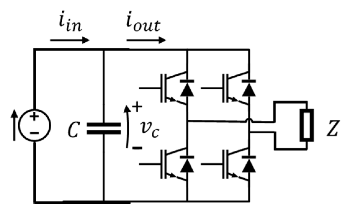
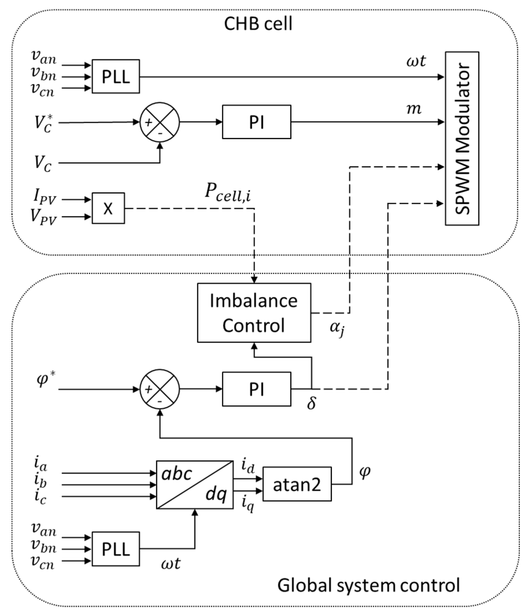
3.1. CHB Cell Control

To control the power delivered by each cell independently, the controller of each CHB cell regulates capacitor voltage by adjusting the modulation index (m) of the H-bridge while MPPT is performed by the isolated DC/DC converter. Furthermore, the control is connected to grid phase voltage measurements to obtain the electric angle (ωt) through a Phase Locked Loop (PLL), as depicted in Figure 3. There is also a communication channel between the cell and global system control. The cells send the power measurement generated by the solar panels (P_cell,i), where “i” is the index referring to each cell, and the global control sends a phase delay (δ) for power factor control and another phase delay (αj) for zero-sequence vector injection, where “j” is the index referring to each phase.

Obtaining the transfer function is necessary for controller design and, as stated previously, the group formed by the solar panels and the isolated DC/DC may be modeled as a current source [26]. Therefore, the equivalent circuit shown in Figure 4 represents a CHB cell.

The magnitude that is compensated is the capacitor mean voltage (〈v_C〉) and the controlling variable is the modulation index (m). In the linear region of the B-SPWM, the amplitude of the voltage generated by the H-bridge, V_HB, is the capacitor mean value multiplied by the modulation index.

$$V_{HB}=m\langle v_C\rangle$$

(1)

Additionally, according to Figure 4, the variation in capacitor voltage can be described by:

$$\frac{d{v}_c\left(t\right)}{dt}=\frac{i_{in}\left(t\right)-i_{out}\left(t\right)}{C},$$

(2)

where v_c is the capacitor voltage, i_in is the input current, i_out is the output current and C is the capacitance. If the mean value is calculated for a fundamental grid period for all the variables, then Equation (2) can be rewritten as:

$$\frac{d\langle v_c\rangle }{dt}=\frac{\langle i_{in}\rangle -\langle i_{out}\rangle }{C},$$

(3)

where 〈v_c〉, 〈i_in〉 and 〈i_out〉 are the mean values of their respective variables. The output current in the AC side is proportional to a sinusoidal waveform while the output current in the DC side may be approximated to the absolute value of the same waveform if the power factor is close to unity. The output current in the AC side can be then expressed as a function of the modulation index (m) and the equivalent resistive load (R_e(Z)), given that the RMS value of the output voltage refers to the modulation index multiplied by the mean DC voltage divided by the square root of 2.

$$i_{out RMS}=\frac{m\langle v_c\rangle }{\sqrt{2}{R}_e\left(Z\right)}$$

(4)

Hence, the mean value of the output current in the DC side may be expressed as:

$$\langle i_{out}\rangle =\frac{2m\langle v_c\rangle }{\pi R_e\left(Z\right)}$$

(5)

Replacing (5) in (3), the variation in capacitor voltage may be expressed as:

$$\frac{d\langle v_c\rangle }{dt}=\frac{\langle i_{in}\rangle }{C}-\frac{2m\langle v_c\rangle }{\pi R_e\left(Z\right)C}$$

(6)

To obtain the small signal model, in a steady state, 〈v_c〉, 〈i_in〉 and m can be expressed according to

$$\langle v_c\rangle =V_c+{\hat{v}}_c$$

(7)

$$\langle i_{in}\rangle =I_{in}+{\hat{i}}_{in}$$

(8)

$$m=M+\hat{m}$$

(9)

where the uppercase variables are the mean values and ${\hat{v}}_c$, ${\hat{i}}_{in}$ and $\hat{m}$ are the small signal perturbations. Introducing (7)–(9) in (6) and neglecting second order terms as follows:

$$\frac{d{V}_c}{dt}=\frac{I_{in}}{C}-\frac{2M{V}_c}{\pi R_e\left(Z\right)C}$$

(10)

$$\frac{d{\hat{v}}_c}{dt}=\frac{{\hat{i}}_{in}}{C}-\frac{2\hat{m} V_c}{\pi R_e\left(Z\right)C}-\frac{ 2{\hat{v}}_{c}M}{\pi R_e\left(Z\right)C}$$

(11)

Equation (10) shows that in a steady state, the mean capacitor voltage value does not change if input and output currents are the same. Furthermore, when applying the Laplace transform to Equation (11), the transfer function of a cell is obtained.

$$G_{vm}\left(s\right)=\frac{{\hat{v}}_c\left(s\right)}{\hat{m}\left(s\right)}=-\frac{2V_c}{2M+\pi R_e\left(Z\right)Cs}$$

(12)

This transfer function represents a first order system with a pole on the left-hand side of the s-plane. Therefore, a PI compensator, as shown in Figure 3, can keep capacitor voltage under control. Due to differences in the power generated by the solar panels of each cell, some authors use an inter-bridge balance submodule to control capacitor voltage [29]. However, with the CHB cell control proposed here, it is not necessary to do so, as each cell can regulate their capacitor voltage without measuring variables from other cells.

3.2. Global System Control

While the cell controller regulates the active power delivered by each cell, the global system control is in charge of performing the power factor control needed to meet the requirements of the grid codes and the imbalance control in order to ensure proper behavior of the converter and prevent any current distortions. The first section explains the power factor control while the second describes the imbalance control.

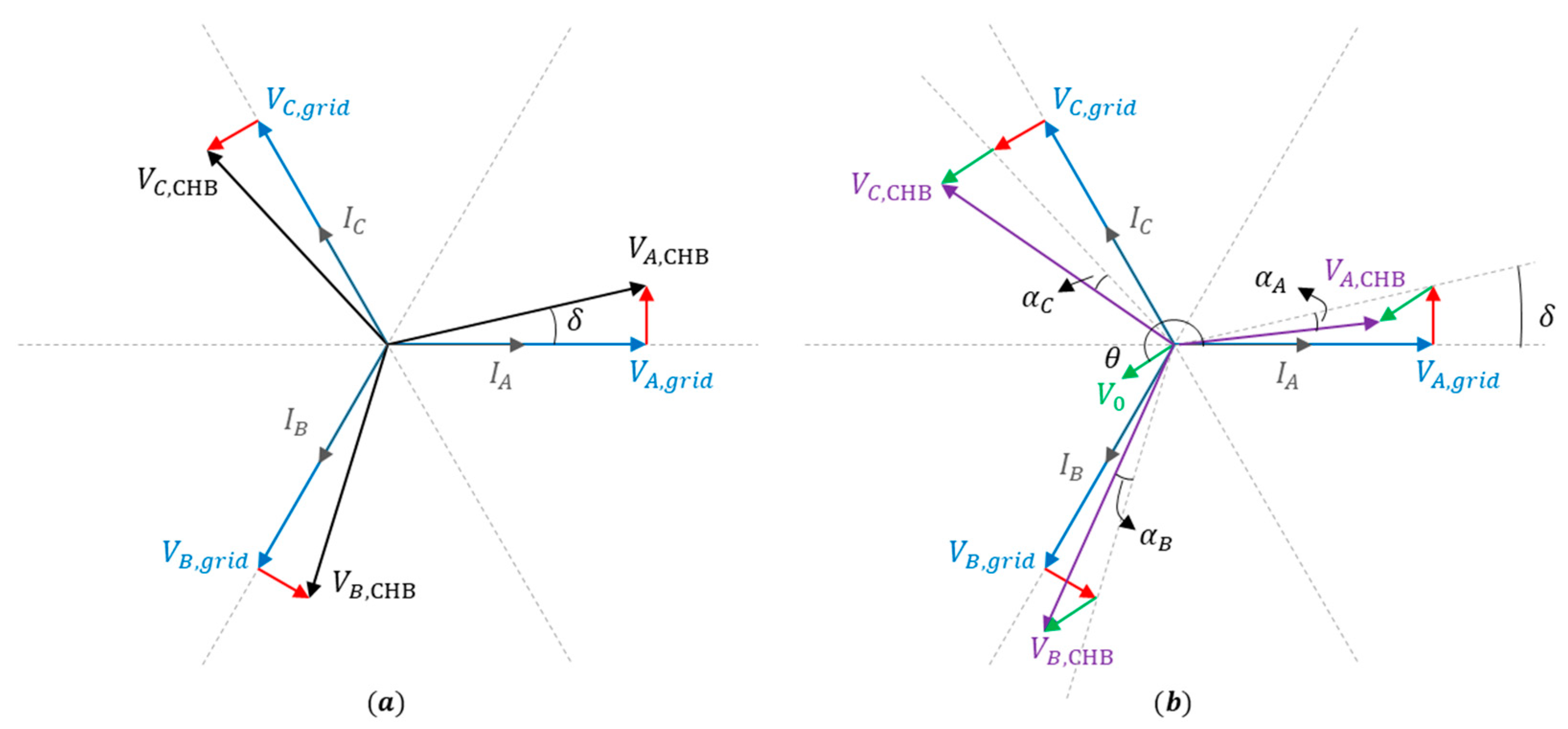
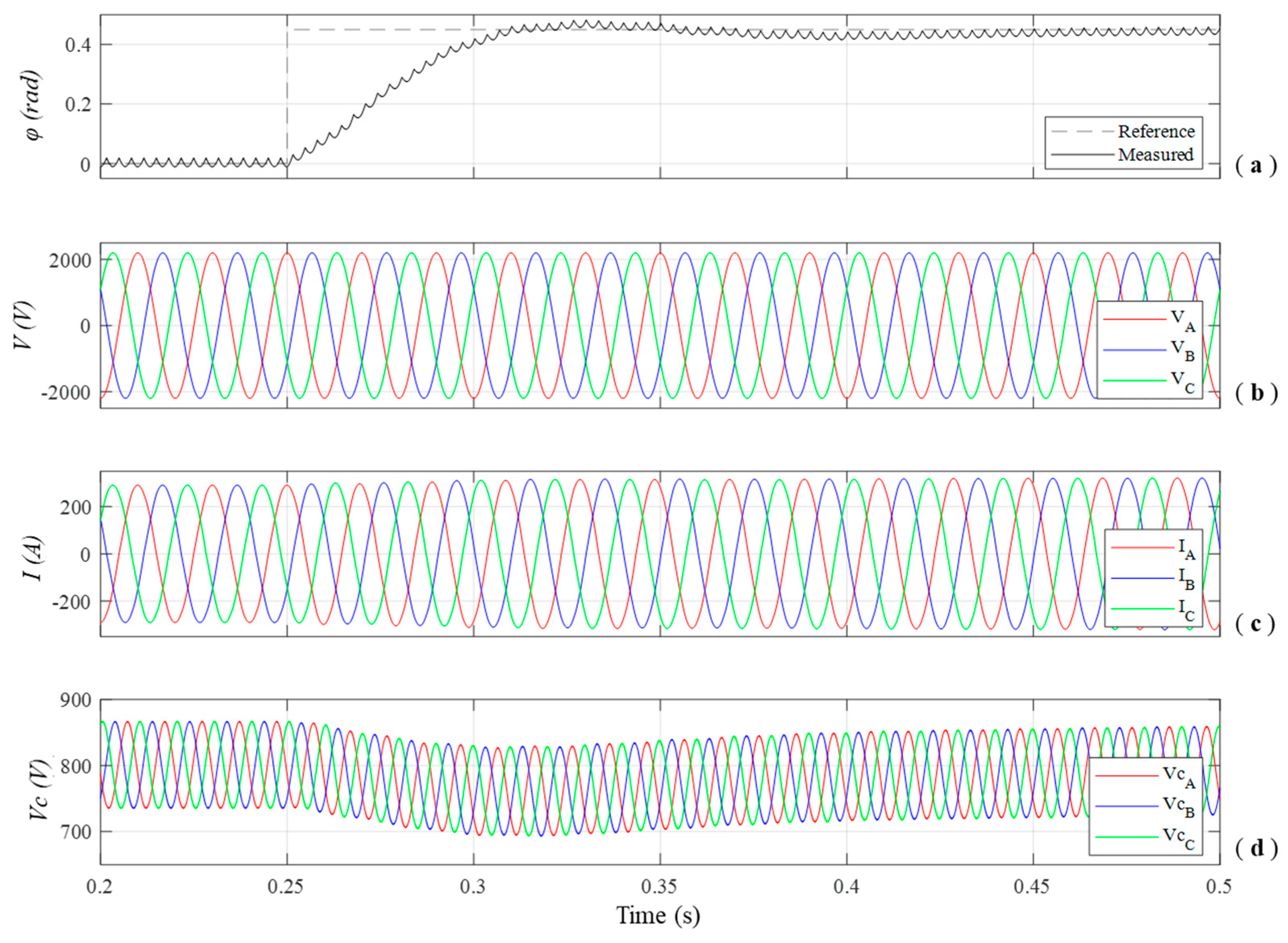
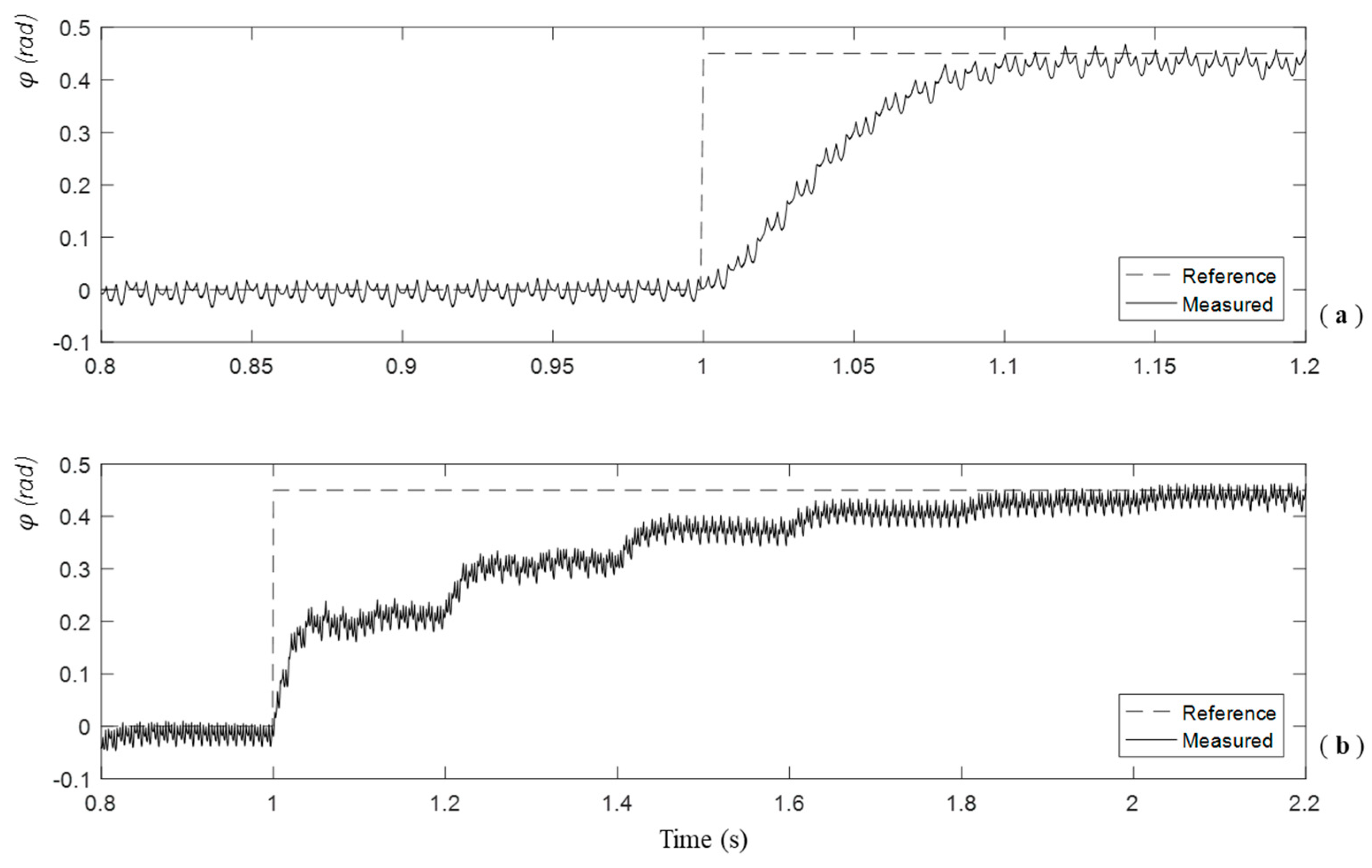
3.2.1. Power Factor Control

As stated previously, the phase delay of the B-SPWM regulates the power factor. A model of a monophasic CHB converter, shown in Figure 5, is analyzed to justify this statement.

A current (i_L) flows through the inductor (L) and the voltages generated by the cells from the CHB converter (v_CHB) and grid (v_grid) can be ideally expressed as:

$$v_{\mathrm{CHB}}\left(t\right)=V_{\mathrm{CHB}}\cos \left(\omega t+\delta \right)$$

(13)

$$v_{grid}\left(t\right)=V_{grid}\cos \left(\omega t\right)$$

(14)

where V_CHB and V_grid are the peak values. Solving the circuit shown in Figure 5, the active power (P) and reactive power (Q) can be described by:

$$P=\frac{V_{\mathrm{CHB}}{V}_{grid}\sin \delta }{\omega L}$$

(15)

$$Q=\frac{V_{grid}}{\omega L}\left(V_{\mathrm{CHB}}\cos \delta -V_{grid}\right)$$

(16)

Equation (16) shows that to control the reactive power, V_CHB must be larger than V_grid, in which case the phase delay (δ) can then control the power factor. Taking into account that the power factor is a global variable and the architecture of the CHB, the phase delay (δ) must be the same for all the CHB cells to ensure all of them are synchronized.

However, according to Equations (15) and (16) and taking into account that the modulation index (m) is directly linked to V_CHB (see Equation (1)), the control variables are not completely decoupled. Therefore, changes in any of them will result in variations in the power factor and active power. Having said this, sizing the cell capacitor properly can minimize the cross-effect to ensure that the control proposed remains valid. Thus, an analysis of how a perturbation in the phase delay affects the capacitor voltage of the cells can determine the capacitance value. By differentiating Equation (15), the power variation due to a variation in the phase delay (δ) is:

$$∆P=\frac{V_{\mathrm{CHB}}{V}_{grid}\cos \delta }{\omega L}∆\delta$$

(17)

For a positive variation in the phase delay (δ), there is an increment in the power delivered to the grid, which means an increment in the RMS value of the current injected into the grid and whit that current increment being:

$$∆i_{out RMS}=\frac{∆P\sqrt{2}}{V_{grid}\cos \phi },$$

(18)

where cos φ is the power factor. In a steady state prior to perturbation, the mean values of the input and output current of the cell capacitor were the same and, consequently, the mean value of the capacitor voltage remained constant.

$$\frac{d\langle v_c\rangle }{dt}=\frac{\langle i_{in}\rangle -\langle i_{out}\rangle }{C}=0$$

(19)

However, due to the increment in the current delivered to the grid, the capacitor voltage mean value drops according to the following equation:

$$\frac{d\langle v_C\rangle }{dt}=\frac{\langle i_{in}\rangle -\langle i_{out}\rangle -\langle ∆i_{out}\rangle }{C}=-\frac{2\sqrt{2}{V}_{\mathrm{CHB}}\cos \delta }{\pi \omega LC\cos \phi }∆\delta$$

(20)

Thus, if the variation takes place during the time interval $∆t$ and allowable voltage drop is $∆V$, the minimum capacitance is:

$$C_{min}=\frac{2\sqrt{2}{V}_{\mathrm{CHB}}\cos \delta }{\pi \omega L\cos \phi }\frac{∆\delta ∆t}{∆V}$$

(21)

To select the appropriate capacitor, the values of V_CHB and δ are calculated from Equations (15) and (16) when the system is operating at nominal power with a power factor of value 1. In addition, the increment in phase delay records the value needed to change the power factor from unity to the minimum allowable value. The capacitor also absorbs the variations in the power delivered by the solar panels and reduces the perturbation caused in the power factor.

To design the power factor controller, the block diagram shown in Figure 6, which represents the system shown in Figure 5 extended to three phases according to [30], is used to obtain the transfer function.

In the block diagram shown in Figure 6, v_{CHB d}, v_{CHB q}, v_{grid_d} and v_{grid_q} are the voltages generated by the converter and the grid expressed in the dq frame, $\omega$ is the grid frequency and $L$ is the grid connection inductor. If the d-axes is aligned with the phase A voltage of the grid and the phase currents (i_A, i_B and i_C) are then given by Equations (22)–(24) as follows:

$$i_A=I_0\cos \left(\omega t+\phi \right),$$

(22)

$$i_B=I_0\cos \left(\omega t-\frac{2\pi }{3}+\phi \right),$$

(23)

$$i_C=I_0\cos \left(\omega t+\frac{2\pi }{3}+\phi \right),$$

(24)

where I₀, is the current amplitude and cos φ is the power factor. Using Clarke’s and Park’s power invariant transformation, the angle formed by dq components of the current (i_d and i_q) is related to the power factor as shown in:

$$\phi ={\tan }^{-1}\left(\raisebox{1ex}{$i_q$}\!\left/ \!\raisebox{-1ex}{$i_d$}\right.\right)$$

(25)

Moreover, with the d-axes is aligned with phase A voltage of the grid, v_{grid_d} and v_{grid_q} may be written as:

$$v_{grid\_d}=V_{grid},$$

(26)

$$v_{grid\_q}=0,$$

(27)

where V_grid is the amplitude of the grid voltage. Expressing the voltage generated by the CHB in the dq frame in terms of voltage amplitude (V_CHB) and phase delay (δ) and taking into consideration Equation (25), the analytical expression of the angle (φ) is:

$$\phi ={\tan }^{-1}\left(\frac{V_{grid}-V_{\mathrm{CHB}}\cos \delta }{V_{\mathrm{CHB}}\sin \delta }\right)$$

(28)

As the modulation indexes of the cells determine voltage amplitude $V_{\mathrm{CHB}}$ in order to control the power generated in each cell, the phase delay is the variable that regulates the power factor. Thus, to obtain the transfer function, Equation (28) is approximated to:

$$\phi \cong {\phi }_0+{\frac{d\phi }{d\delta }|}_{{\delta }_0}\left(\delta -{\delta }_0\right),$$

(29)

where φ₀ and δ₀ are the angles at a determined operating point. In a steady state, φ and δ can be expressed according to the following equations.

$$\phi ={\phi }_0+\hat{\phi }$$

(30)

$$\delta ={\delta }_0+\hat{\delta }$$

(31)

Replacing Equations (30) and (31) in Equation (29) and evaluating the derivative at point δ₀ leads to the transfer function being obtained as follows:

$$G_{\phi \delta }\left(s\right)=\frac{\widehat{\phi }\left(s\right)}{\hat{\delta }\left(s\right)}=\frac{V_{\mathrm{CHB}}^2-V_{\mathrm{CHB}}{V}_{grid}\cos {\delta }_0}{V_{\mathrm{CHB}}^2-2V_{\mathrm{CHB}}{V}_{grid}\cos {\delta }_0+V_{grid}^2}$$

(32)

The resulting transfer function is a gain and, consequently, the stability and transient response of the closed loop system depends on the poles of the PI controller. Furthermore, as the power factor control needs a communication channel (see Figure 3), discretization time plays a key role in the control strategy and determines the specifications of the communication protocol. According to the transfer function of Equation (32) in the discrete case, the PI controller also determines the transient response and stability of the closed loop system. However, the influence of the discretization time is verified in the simulation section.

3.2.2. Imbalance Control

In photovoltaic applications, several factors can lead to unequal power generation in CHB cells [31]. The imbalances that may occur inside each phase are compensated by CHB cell control, but this cannot compensate imbalances between phases that cause distortions in the currents injected into the grid. The zero-sequence vector injection proposed in [24] solves this problem by redistributing the power generated among the three phases. However, the control method proposed in this paper cannot apply the zero-sequence vector injection in the same way as in [24] and so an alternative solution is proposed. In the control method proposed, the global system control cannot establish the module of the phasors that represent the voltage generated by the converter because CHB cell control performs that task. Nevertheless, the global system control method determines the direction of each vector based on the power generated by each cell, grid voltage and phase delay ($\delta$), which refers to the output of the power factor controller. Thus, for the scalable control method proposed, zero-sequence vector injection requires modifications in order to calculate the direction of each vector.

To explain these modifications, Figure 7a shows the phasor diagram under normal operation, i.e., when the power generated by the solar panels of each phase is the same, while Figure 7b shows the phasor diagram after zero-sequence vector injection once the power generated by the solar panels of each phase is different. This case is equal to the scenario described in [24], where the power generated in phase A (P_A) is lower than that generated in phase C (P_C), which is in turn lower than that generated in phase B (P_B). This implies that voltage amplitudes will be different as well. The system gets balanced because the zero-sequence vector allows power exchange between phases. To achieve balanced operation under imbalanced circumstances the zero sequence vector is added to ideal vectors of an equivalent normal operation scenario, Figure 7a, leading to the scenario depicted in Figure 7b.

According to [24], the zero-sequence vector can be calculated as:

$$\left|V_0\right|=\frac{V_{grid}}{2\sqrt{2}{P}_{avg}}\sqrt{{\left(P_A-P_B\right)}^2+{\left(P_B-P_C\right)}^2+{\left(P_C-P_A\right)}^2}$$

(33)

$$\theta ={\tan }^{-1}\left(\frac{\sqrt{3}\left(P_C-P_B\right)}{2P_A-P_B-P_C}\right)$$

(34)

where V_grid denotes the peak value of the phase-to-neutral voltage and P_avg is the mean power generated by the solar panels of the three phases. Hence, by adding the vector V₀ to vectors V_A,CHB, V_B,CHB and V_C,CHB of Figure 7a and taking into account their relationships with the phase delay (δ) and grid voltage, the resulting vectors shown in Figure 7b can be expressed as:

$$V_{Ax,\mathrm{CHB}}=V_0\cos \theta +V_{grid}$$

(35)

$$V_{Ay,\mathrm{CHB}}=V_0\sin \theta +V_{grid}\tan \delta$$

(36)

$$V_{Bx,\mathrm{CHB}}=V_0\cos \theta -\frac{1}{2}{V}_{grid}+\frac{\sqrt{3}}{2}{V}_{grid}\tan \delta$$

(37)

$$V_{By,\mathrm{CHB}}=V_0\sin \theta -\frac{\sqrt{3}}{2}{V}_{grid}-\frac{1}{2}{V}_{grid}\tan \delta$$

(38)

$$V_{Cx,\mathrm{CHB}}=V_0\cos \theta -\frac{1}{2}{V}_{grid}-\frac{\sqrt{3}}{2}{V}_{grid}\tan \delta$$

(39)

$$V_{Cy,\mathrm{CHB}}=V_0\sin \theta +\frac{\sqrt{3}}{2}{V}_{grid}-\frac{1}{2}{V}_{grid}\tan \delta$$

(40)

Consequently, the phase delay $\left({\alpha }_j\right)$ sent to each phase may be written as:

$${\alpha }_A={\tan }^{-1}\left(\raisebox{1ex}{$V_{Ay,\mathrm{CHB}}$}\!\left/ \!\raisebox{-1ex}{$V_{Ax,\mathrm{CHB}}$}\right.\right)-\delta$$

(41)

$${\alpha }_B={\tan }^{-1}\left(\raisebox{1ex}{$V_{By,\mathrm{CHB}}$}\!\left/ \!\raisebox{-1ex}{$V_{Bx,\mathrm{CHB}}$}\right.\right)-\delta +\frac{2\pi }{3}$$

(42)

$${\alpha }_C={\tan }^{-1}\left(\raisebox{1ex}{$V_{Cy,\mathrm{CHB}}$}\!\left/ \!\raisebox{-1ex}{$V_{Cx,\mathrm{CHB}}$}\right.\right)-\delta -\frac{2\pi }{3}$$

(43)

As a result, the system can provide a balanced operation in an unequal power generation scenario if the global system control method receives information about the power generated in each cell and sends the phase delay $\left({\alpha }_j\right)$ to each cell in order to inject the corresponding zero-sequence vector. The power measurements of each cell will vary as the irradiation received by the solar panels varies, although this phenomenon is slow compared to a typical communication channel bit rate.

To sum up, this section fully describes the scalable control strategy proposed, including all the blocks that form the control scheme shown in Figure 3. CHB cell control regulates active power, which takes place in each cell, whereas the global system control method regulates the power factor and makes zero-sequence vector injection possible in order to compensate for any phase imbalances.

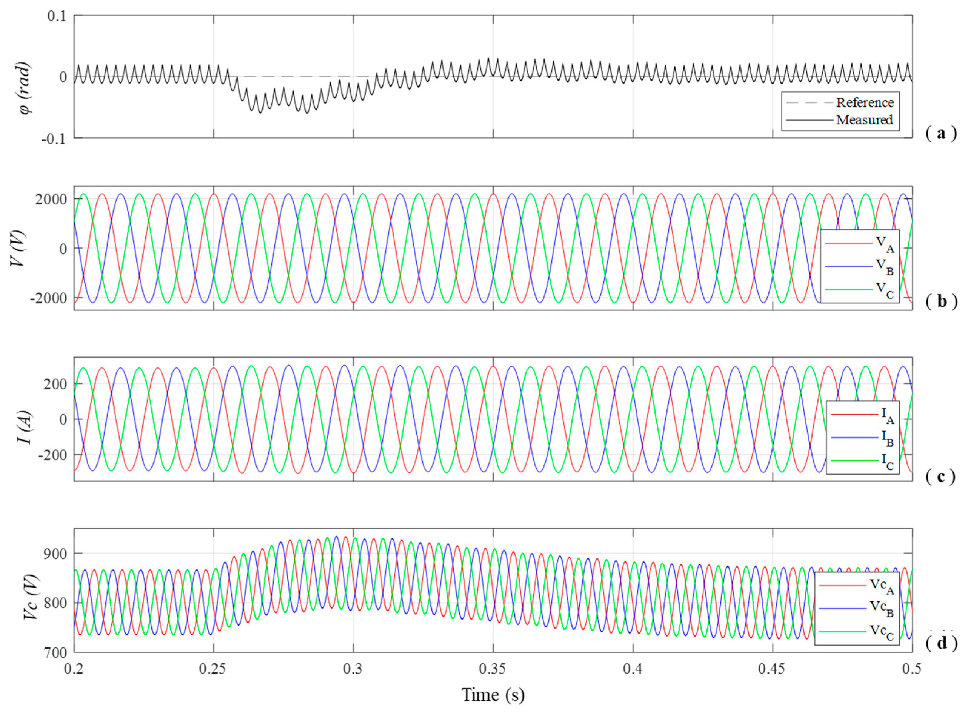
4. Results and Discussion

The aim of this section is to validate the control strategy by conducting simulations on an illustrative downsized 12 H-bridge model using PSIM (Powersim). Firstly, power factor control and CHB cell control are analyzed. Afterwards, the communication requirements are studied and, finally, the zero-sequence vector injection is tested.

4.1. Power Factor Control and CHB Cell Control Validation

Validation of power factor control and CHB cell control takes place in two different scenarios. In the first, each cell generates 80 kW and the power factor reference changes from 1 to 0.9, which is the minimum power factor allowed in this case. In the second scenario, the power factor reference is 1 and the cells generate 80 kW each when one cell from each phase starts to generate 88 kW instantaneously. In the case of both scenarios,

Table 1. PSIM simulation parameters.

Simulation Parameters	Value
L (mH)	5
f (Hz)	50
fs (kHz)	10
C (mF)	2.5
V*C (V)	800
Vgrid (V)	2200

summarizes the parameters included in the simulation.

Capacitor size is selected considering that at nominal power of 960 kW and with a power factor of value 1, voltage $V_{\mathrm{CHB}}$ records the theoretical value of 2212 V and phase delay $\delta$ is 0.1042 rad, according to Equations (15) and (16). Changing the power factor from 1 to 0.9 means a variation in phase delay of 0.004 rad. However, as the phase delay does not change instantaneously, the maximum phase delay increment ($∆\delta$) allowed is 0.002 rad over 50 ms. Thus, Equation (21) establishes a minimum capacitance of 2.5 mF to limit voltage drop to 50 V. This value guarantees that the available DC voltage bus of each phase will be greater than the grid voltage amplitude during transient time.

In the first scenario, the system tracks the angle that determines the power factor and the transition takes place smoothly, as can be seen in Figure 8a–c, in which the reference tracking, grid voltages and injected currents are shown, respectively. Additionally, Figure 8d shows a perturbation in capacitor voltage that demonstrates that the control variables are not totally decoupled, as explained in the power factor control section. However, the perturbation does not affect system performance while the controllers are working independently because capacitor value limits the voltage drop to less than 35 V, which is less than 5% of the reference value. This, in turn, is better than the approximation because of the CHB cell controller action.

In case of the second scenario, where the power factor reference is 1, the cells generate 80 kW each and one cell from each phase starts to generate 88 kW instantaneously. Figure 9 shows that the power increment has little effect on power factor control, even though the former is instantaneous. Indeed, the perturbation affects capacitor voltage more, considering that voltage mean value rises to around 50 V whereas the maximum error in the angle tracking is 0.06 rad, which means a power factor of 0.9982, less than 1% error. Moreover, the power factor recovers the reference value faster than the capacitor voltage. The capacitor voltages shown in Figure 9d correspond to the cells with the power increment because they show perturbations while the mean value of the capacitor voltage of other cells remains constant.

Thus, despite the fact that the control variables are not completely decoupled, power factor control and CHB cell control can operate as if they were decoupled in these kinds of applications. Additionally, these results show that the control strategy proposed has an equivalent behavior to VOC-based strategies described in [9,10,11].

4.2. Communication Requirements

Due to data exchange between the controllers, communication channel requirements are the limiting factor of the scalability of the control strategy. Hence, the influence of discretization time in the power factor controller determines the transmission rate of the communication channel. To observe the effect of discretization time, the simulations of the first scenario are repeated with discretized controllers to ensure power factor control. Discretization times are 10 ms and 100 ms because they are typical transmission periods in CAN communication channels, with Figure 10a,b showing the step responses for discretization times of 10 ms and 100 ms, respectively.

The responses are stable and slower than in the continuous case as expected, taking into consideration the transfer function shown in Equation (32). There is a wide range available from which to choose the transmission rate according to the number of cells. Furthermore, while the data received by global control grows linearly as the number of cells grows, the data transmitted via global control to the cells is independent of the number of cells, which improves scalability and removes the size limitation of the strategy proposed in [23]. Additionally, the wide range of transmission period allows for using a communication protocol less demanding than the control methods proposed in [21,22].

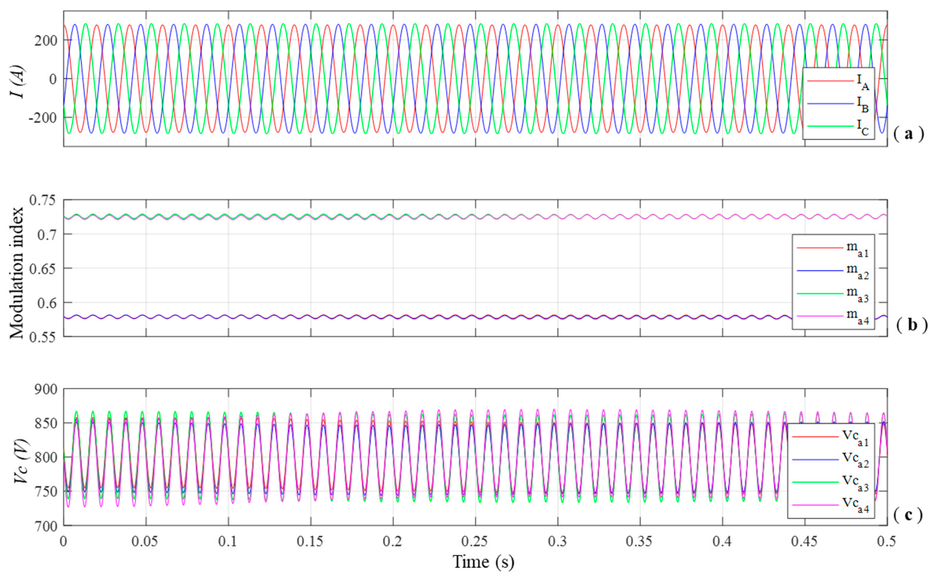
4.3. Zero-Sequence Vector Injection

For validation of the zero-sequence vector injection, the simulation represents an unequal power generation scenario that might be caused by a partial shading of the photovoltaic panels in a section of the power plant. The scenario consists of two cells from phase A (a₁ and a₂) that generate 64 kW while the other two from phase A (a₃ and a₄) and those from phases B and C generate 80 kW. In a steady state, the angular variables δ, α_A, α_B and α_C record values of 0.1593 rad, 0.0084 rad, −0.0489 rad and 0.0407 rad, respectively.

Additionally, Figure 11a shows that three phases share the power evenly among them and keep the injected currents balanced in an unequal power scenario, while Figure 11b,c proves that each cell can adjust their modulation index to regulate the power delivered via the control strategy proposed, keeping the capacitor voltage stable. Therefore, it is not necessary to use an inter-module balancing controller that reduces the scalability dramatically and control strategy proposed is able to implement the zero-sequence vector injection technique described in [24] correctly.

5. Conclusions

Until now, the control strategies that appear in literature have not been able to take advantage of the modularity feature of CHB inverters because control methods require too many signals or rely on complex communication protocols. The present paper describes a scalable control strategy for CHB converters in photovoltaic applications based on sinusoidal modulation instead of vector modulation. The method proposed regulates different aspects of the converter independently dividing the control into two different compensators, which improves scalability of the CHB topology. The first is CHB cell control that regulates the active power delivered by each cell by adjusting the modulation index, which is calculated in terms of internal magnitudes. The other controller is the global system control that regulates the power factor and any inter-phase imbalances. The power factor control method uses phase delay as a control variable and transmits the phase delay to the cells.

The simulation results show that the scalable strategy proposed is capable of controlling a photovoltaic power plant under imbalanced circumstances. Discretization time mainly influences the rise and stabilization time and, as shown in the simulation results, the value of the discretization time is high enough for the use of a high-speed communication protocol not to be mandatory. Indeed, a CAN communication network could be used for the present application. Furthermore, the value of the phase delay is the same in the case of all cells, which is significantly different from what papers state about distributed control of CHB inverters and improves greatly the scalability feature. The perturbations that appear during a change of power factor are also controlled with the cell capacitors so that they will not affect the behavior of the whole system.

To sum up, the distributed control strategy presented here constitutes an effective way of taking full advantage of CHB modularity. The communication requirements are far less demanding than in previous works because of the novel control strategy. Moreover, the control method can be easily implemented in commonly used DSPs and may help to improve the performance of large-scale solar power plants in the future.

References

1. International Renewable Energy Agency Abu Dhabi. Renewable Generation Costs 2018; IRENA: Masdar City, Abu Dhabi, 2019. [Google Scholar]
2. Albright, G.; Edie All Cell Technologies; Crossley, P.; Vassallo, A. Battery Storage Report; IRENA: Masdar City, Abu Dhabi, 2015. [Google Scholar]
3. Ram, M.; Aghahosseini, A.; Breyer, C. Job creation during the global energy transition towards 100% renewable power system by 2050. Technol. Forecast. Soc. Chang. 2020, 151, 119682. [Google Scholar] [CrossRef]
4. Sher, H.A.; Addoweesh, K.E.; Al-Haddad, K. An Efficient and Cost-Effective Hybrid MPPT Method for a Photovoltaic Flyback Microinverter. IEEE Trans. Sustain. Energy 2018, 9, 1137–1144. [Google Scholar] [CrossRef]
5. Kim, H.; Lee, J.S.; Lai, J.-S.; Kim, M. Iterative learning controller with multiple phase-lead compensation for dual-mode flyback inverter. IEEE Trans. Power Electron. 2017, 32, 6468–6480. [Google Scholar] [CrossRef]
6. Ding, M.; Xu, Z.; Wang, W.; Wang, X.; Song, Y.; Chen, D. A review on China’s large-scale PV integration: Progress, challenges and recommendations. Renew. Sustain. Energy Rev. 2016, 53, 639–652. [Google Scholar] [CrossRef]
7. Kouro, S.; Malinowski, M.; Gopakumar, K.; Pou, J.; Franquelo, L.G.; Wu, B.; Rodriguez, J.; Perez, M.A.; Leon, J.I. Recent Advances and Industrial Applications of Multilevel Converters. IEEE Trans. Ind. Electron. 2010, 57, 2553–2580. [Google Scholar] [CrossRef]
8. Rivera, S.; Kouro, S.; Wu, B.; Leon, J.I.; Rodriguez, J.; Franquelo, L.G. Cascaded H-bridge multilevel converter multistring topology for large scale photovoltaic systems. In Proceedings of the 2011 IEEE International Symposium on Industrial Electronics, Gdansk, Poland, 27–30 June 2011; pp. 1837–1844. [Google Scholar] [CrossRef] [Green Version]
9. Wang, K.; Zhu, R.; Wei, C.; Liu, F.; Wu, X.; Liserre, M. Cascaded Multilevel Converter Topology for Large-Scale Photovoltaic System with Balanced Operation. IEEE Trans. Ind. Electron. 2019, 66, 7694–7705. [Google Scholar] [CrossRef]
10. Xiao, B.; Hang, L.; Mei, J.; Riley, C.; Tolbert, L.; Ozpineci, B. Modular Cascaded H-Bridge Multilevel PV Inverter With Distributed MPPT for Grid-Connected Applications. IEEE Trans. Ind. Appl. 2015, 51, 1722–1731. [Google Scholar] [CrossRef]
11. Marks, N.D.; Summers, T.J.; Betz, R.E. Reactive power requirements for cascaded H-Bridge photovoltaic systems. In Proceedings of the IECON 2014—40th Annual Conference of the IEEE Industrial Electronics Society 2014, Dallas, TX, USA, 29 October–1 November 2014; pp. 2219–2225. [Google Scholar] [CrossRef]
12. Mateus, T.H.D.A.; Pomilio, J.A.; Godoy, R.B.; Pinto, J.O.P. Distributed MPPT scheme for grid connected operation of photovoltaic system using cascaded H-bridge multilevel converter under partial shading. In Proceedings of the 2017 IEEE Southern Power Electronics Conference (SPEC) 2017, Puerto Varas, Chile, 4–7 December 2017; pp. 1–6. [Google Scholar] [CrossRef]
13. Cortes-Vega, D.; Alazki, H. Robust maximum power point tracking scheme for PV systems based on attractive ellipsoid method. Sustain. Energy Grids Netw. 2021, 25, 100410. [Google Scholar] [CrossRef]
14. Malinowski, M.; Kazmierkowski, M.P.; Trzynadlowski, A. A comparative study of control techniques for PWM rectifiers in AC adjustable speed drives. IEEE Trans. Power Electron. 2003, 18, 1390–1396. [Google Scholar] [CrossRef]
15. Haji-Esmaeili, M.M.; Naseri, M.; Khoun-Jahan, H.; Abapour, M. Fault-tolerant structure for cascaded H-bridge multilevel inverter and reliability evaluation. IET Power Electron. 2017, 10, 59–70. [Google Scholar] [CrossRef]
16. Wang, C.; Zhang, K.; Xiong, J.; Xue, Y.; Liu, W. An Efficient Modulation Strategy for Cascaded Photovoltaic Systems Suffering From Module Mismatch. IEEE J. Emerg. Sel. Top. Power Electron. 2018, 6, 941–954. [Google Scholar] [CrossRef]
17. Stonier, A.A.; Lehman, B. An Intelligent-Based Fault-Tolerant System for Solar-Fed Cascaded Multilevel Inverters. IEEE Trans. Energy Convers. 2018, 33, 1047–1057. [Google Scholar] [CrossRef]
18. Baimel, D. Implementation of DQ0 control methods in high power electronics devices for renewable energy sources, energy storage and FACTS. Sustain. Energy Grids Netw. 2019, 18, 100218. [Google Scholar] [CrossRef]
19. Li, B.; Yang, R.; Xu, D.; Wang, G.; Wang, W.; Xu, D. Analysis of the Phase-Shifted Carrier Modulation for Modular Multilevel Converters. IEEE Trans. Power Electron. 2015, 30, 297–310. [Google Scholar] [CrossRef]
20. Kouro, S.; Wu, B.; Moya, A.; Villanueva, E.; Correa, P.; Rodriguez, J. Control of a cascaded H-bridge multilevel converter for grid connection of photovoltaic systems. In Proceedings of the 2009 35th Annual Conference of IEEE Industrial Electronic, Porto, Portugal, 3–5 November 2009; pp. 3976–3982. [Google Scholar] [CrossRef]
21. Mathe, L.; Burlacu, P.D.; Teodorescu, R. Control of a Modular Multilevel Converter with Reduced Internal Data Exchange. IEEE Trans. Ind. Inform. 2017, 13, 248–257. [Google Scholar] [CrossRef]
22. McGrath, B.P.; Holmes, D.G.; Kong, W.Y. A Decentralized controller architecture for a cascaded H-bridge multilevel converter. IEEE Trans. Ind. Electron. 2014, 61, 1169–1178. [Google Scholar] [CrossRef]
23. Wu, P.-H.; Su, Y.-C.; Shie, J.-L.; Cheng, P.-T. A Distributed Control Technique for the Multilevel Cascaded Converter. IEEE Trans. Ind. Appl. 2019, 55, 1649–1657. [Google Scholar] [CrossRef]
24. Yu, Y.; Konstantinou, G.; Hredzak, B.; Agelidis, V.G. Operation of Cascaded H-Bridge Multilevel Converters for Large-Scale Photovoltaic Power Plants under Bridge Failures. IEEE Trans. Ind. Electron. 2015, 62, 7228–7236. [Google Scholar] [CrossRef]
25. Buccella, C.; Cecati, C.; Latafat, H.; Razi, K. A grid-connected PV system with LLC resonant DC-DC converter. In Proceedings of the 2013 International Conference on Clean Electrical Power (ICCEP), Alghero, Italy, 11–13 June 2013; pp. 777–782. [Google Scholar] [CrossRef]
26. Sochor, P.; Akagi, H. Theoretical comparison in energy-balancing capability between star- and delta-configured modular multilevel cascade inverters for utility-scale photovoltaic systems. IEEE Trans. Power Electron. 2016, 31, 1980–1992. [Google Scholar] [CrossRef]
27. De Kooning, J.; Van De Vyver, J.; De Kooning, J.D.; VanDoorn, T.L.; Vandevelde, L. Grid voltage control with distributed generation using online grid impedance estimation. Sustain. Energy Grids Netw. 2016, 5, 70–77. [Google Scholar] [CrossRef]
28. Khluabwannarat, P.; Thammarat, C.; Tadsuan, S.; Bunjongjit, S. An analysis of iron loss supplied by sinusoidal, square wave, bipolar PWM inverter and unipolar PWM inverter. In Proceedings of the 8th International Power Engineering Conference, IPEC, Singapore, 3–6 December 2007; pp. 1185–1190. [Google Scholar]
29. Liang, G.; Tafti, H.D.; Farivar, G.G.; Pou, J.; Townsend, C.D.; Konstantinou, G.; Ceballos, S. Analytical Derivation of Intersubmodule Active Power Disparity Limits in Modular Multilevel Converter-Based Battery Energy Storage Systems. IEEE Trans. Power Electron. 2021, 36, 2864–2874. [Google Scholar] [CrossRef]
30. Gataric, S.; Garrigan, N. Modeling and design of three-phase systems using complex transfer functions. PESC Rec. IEEE Annu. Power Electron. Spec. Conf. 1999, 2, 691–697. [Google Scholar]
31. Essakiappan, S.; Krishnamoorthy, H.S.; Enjeti, P.; Balog, R.S.; Ahmed, S. Multilevel Medium-Frequency Link Inverter for Utility Scale Photovoltaic Integration. IEEE Trans. Power Electron. 2015, 30, 3674–3684. [Google Scholar] [CrossRef]
Figure 1. Grid tied CHB inverter in a photovoltaic plant.
Energies 15 00208 g001
Figure 2. VOC control with zero-sequence vector injection for a generic CHB grid-tied converter.
Energies 15 00208 g002
Figure 3. Control scheme proposed.
Energies 15 00208 g003
Figure 4. Equivalent circuit of a CHB cell.
Energies 15 00208 g004
Figure 5. Model of a monophasic CHB grid-tied inverter.
Energies 15 00208 g005
Figure 6. Block diagram of a three-phase inductor in the dq frame.
Energies 15 00208 g006
Figure 7. (a) Phasor diagram for normal operation; (b) Phasor diagram for unequal power generation (Pa < Pc < Pb).
Energies 15 00208 g007
Figure 8. (a) Angle tracking, (b) grid phase-to-neutral voltages, (c) injected currents and (d) capacitor voltage of one cell of each phase in the first scenario.
Energies 15 00208 g008
Figure 9. (a) Angle tracking, (b) grid phase-to-neutral voltages, (c) injected currents and (d) capacitor voltage of cells with a power increment in the second scenario.
Energies 15 00208 g009
Figure 10. Angle tracking for discretization time of (a) 10 ms and (b) 100 ms.
Energies 15 00208 g010
Figure 11. (a) Injected currents, (b) modulation indexes and (c) capacitor voltage of cells from phase A in an unequal power generation scenario.
Energies 15 00208 g011