Model Reference Adaptive Control and Fuzzy Neural Network Synchronous Motion Compensator for Gantry Robots

Abstract

A model reference adaptive control and fuzzy neural network (FNN) synchronous motion compensator for a gantry robot is presented in this paper. This paper proposes the development and application of gantry robots with MRAC and FNN online compensators. First, we propose a model reference adaptive controller (MRAC) under the cascade control method to make the reference model close to the real model and reduce tracking errors for the single axis. Then, a fuzzy neural network compensator for the gantry robot is proposed to compensate for the synchronous errors between the dual servo motors to improve precise movement. In addition, an online parameter training method is proposed to adjust the parameters of the FNN. Finally, the experimental results show that the proposed method improves the synchronous errors of the gantry robot and demonstrates the methodology in this paper. This study also successfully integrates the hardware and successfully verifies the proposed methods.

1. Introduction

Gantry robots have been widely used in manufacturing industries such as high-precision motion control, precision manufacturing, circuit assembly, microelectronics, and inspection [1,2,3]. The gantry robot is composed of a manipulator on an overhead system, and two motors are installed on two parallel linear guides to drive the moving platform. However, due to various factors, such as unbalanced forces on both sides, various disturbances in the driving process will cause synchronous errors between the two motors. The consequence of these synchronous errors will not only cause system jitter and affect the quality of the workpiece but also cause the work process to stop due to overcurrent protection. These undesirable effects are very much in need of control and improvement for high-speed and high-precision manufacturing. Therefore, how to effectively control the synchronous errors of a gantry position platform has become a key issue.

Typical methods (see Figure 1) to synchronize the motion in gantry robot control systems include (1) the cascade control method, and (2) the parallel control method [4,5]. Both methods use two control loops to control the motors separately. The first control method divides the two control loops into a master loop and a slave loop, and the reference command is only provided to the master loop. The master loop has a master motor, and the slave loop has a slave motor. If the master loop encounters a disturbance, the slave loop also reflects the disturbance. The second control method has the two control loops follow the same reference position command. Since the inevitable differences between the two subsystems (including motors, motor drives, etc.) are not taken into account, this method usually exhibits poor performance.

Recently, compensators [6,7,8,9] and cross-coupling technology have often been used in machine tools and multiaxis motion applications [10,11] to solve synchronization control problems and improve control performance [12,13,14,15]. In cross-coupling control, each loop also considers the position and speed errors of another motor to evaluate its own control performance. However, these methods cannot provide sufficient robustness because the control parameters are selected through trial and error.

Fuzzy neural networks (FNNs) [16,17,18,19,20,21,22,23,24,25,26] is an intelligent technology that combines the advantages of fuzzy logic and neural network systems. The FNN system is a straightforward implementation of a fuzzy inference system with a four-layered network structure. Generally, the advantage of FNN systems lies in that: (1) the FNN system can automatically identify fuzzy logic rules, (2) the parameters of the FNN system have clear physical meanings, (3) the FNN system can incorporate linguistic information (in the form of fuzzy IF-THEN rules), and (4) the desired performance can be obtained under fewer adjustable parameters than in neural networks. Generally, FNNs can be divided into the Mamdani type and Takagi–Sugeno–Kang (TSK) type. Since the TSK model can incorporate mathematical knowledge about the controlled plant and can use control theory to analyse its behaviour, the TSK model is the most commonly used FNN method.

Recent research on gantry robots, such as literature [27], discusses the synchronous control based on fuzzy single neuron PID cross-coupling controller, literature [28] discusses the suppression of the rotational motion of cross-coupled gantry stage and literature [29] proposes a new algorithm to identify the parameters of the synchronous dual-drive ball screw gantry system. This paper proposes the development and application of gantry robots with MRAC and FNN online compensators. For the controller design, a cascade control method with an MRAC controller is proposed to ensure the tracking requirements of single axis control. Then, the purpose of the FNN compensator is to eliminate the synchronous errors between the dual servo motors. To improve the learning ability of FNN, an online parameter training method is proposed to adjust the parameters of the FNN. This paper has developed and successfully completed the theoretical and technical feasibility of the proposed method through various experimental comparisons.

The rest of the paper is organized as follows. The gantry robot servo system description is given in Section 2. Section 3 presents the proposed synchronous control methods of gantry robots. The FNN online compensator with two inputs and one output is developed to compensate for the synchronous errors. The experimental results are illustrated in Section 4 to demonstrate the methodology proposed in this paper.

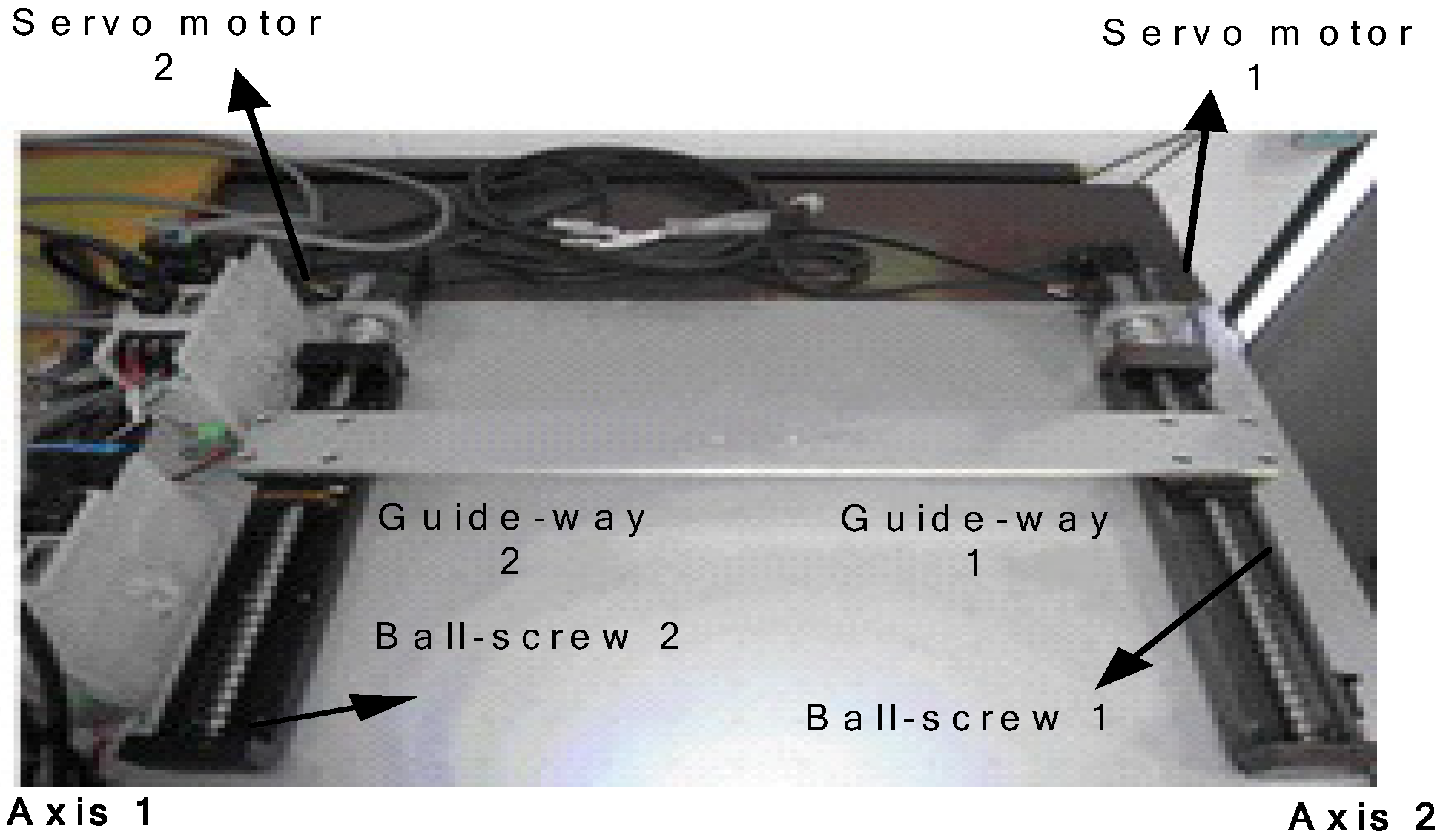
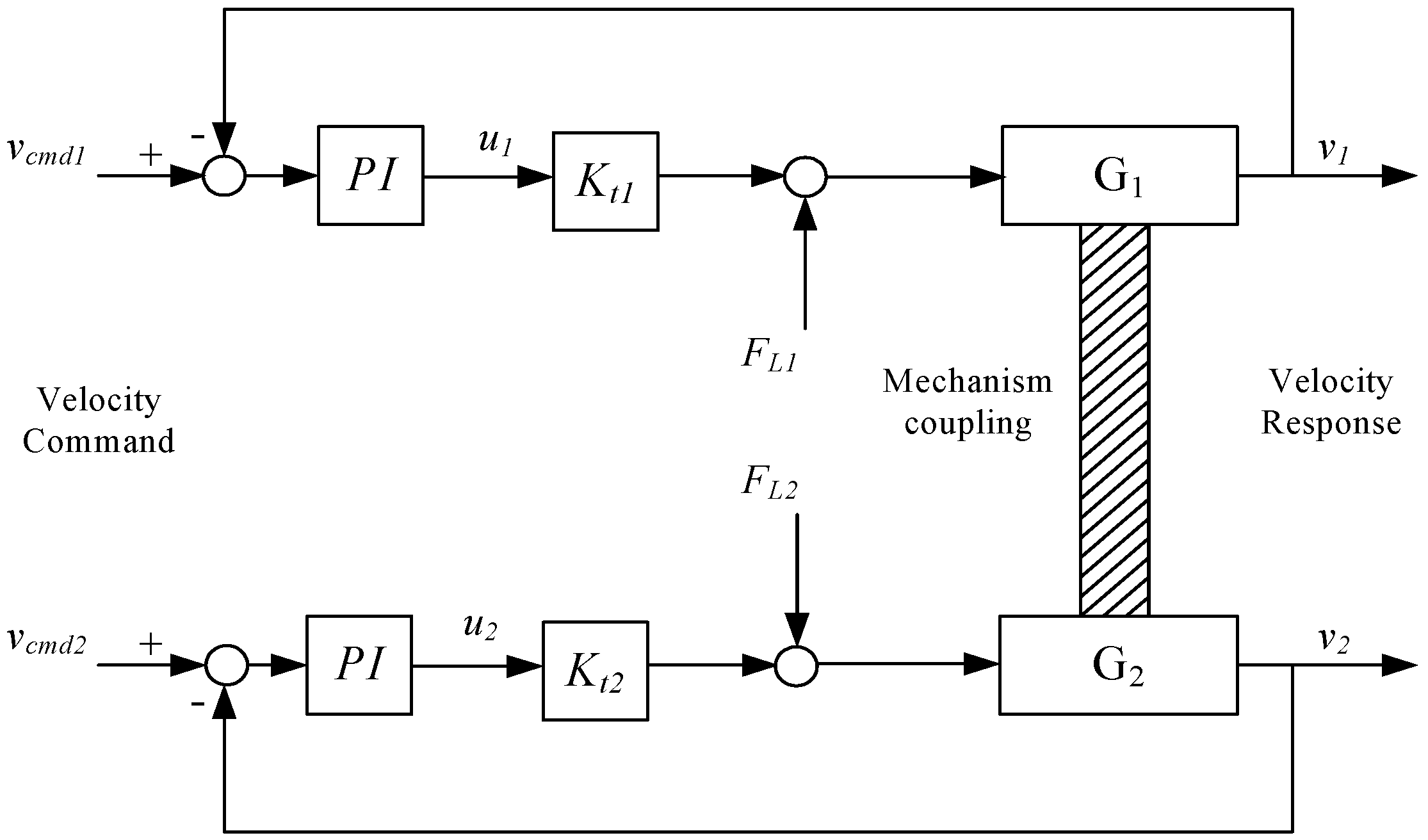
2. The Structure and Mathematical Model of the Gantry Robot System

Figure 2 shows the gantry robot system used in this paper. It consists of two rotating servo motors, guideways, and ball screws.

In traditional cascade control, the inner current control loop usually has a high gain to minimize the current error over the system operating range. The bandwidth of the current loop is usually well over 2 kHz, and the effect of back EMF is eliminated. The electronic dynamics are so fast that the transfer function of the AC servo drive can be treated as a constant current gain. For simplicity, the system equations of each axis of the gantry robot can be shown as

$$M_i{\dot{v}}_i+D_i{v}_i+F_{Li}=K_{ti}{u}_i$$

(1)

where $M_i$ is the equivalent mass of the mechanism; $D_i$ is the equivalent viscous friction; $K_{ti}$ is the torque constant; $F_{Li}$ is the external disturbance term; and u_i is the control effort. Then, the undermined plant is

$$G_i\left(s\right)=\frac{v_i}{K_{ti}{u}_i-F_{Li}}=\frac{1}{M_{i}s+D_i}$$

(2)

The velocity PI controller (shown in Figure 3) is used to eliminate external disturbances. Then, the identified plant from the control effort to the velocity response can be simplified to

$$\frac{v_i}{u_i}=K_{ti}{G}_i\left(s\right)=\frac{K_{ti}}{M_{i}s+D_i}=\frac{K_i}{{\tau }_{i}s+1}$$

(3)

Then, the input command, shown in Figure 4a, is simultaneously fed into each axis as v_cmd1 and v_cmd2, and the responses of Axes 1 and 2 are shown in Figure 4b. The data of Figure 4a,b are utilized to identify the parameters in Equation (3); then, the identified results of each axis are indicated in

Table 1. Identified parameters of gantry stage.

Gain	Value	Time Constant	Value
$K_1(\raisebox{1ex}{$mm$}\!\left/ \!\raisebox{-1ex}{$\mathrm{s}\cdot volt$}\right.)$	393.79	${\tau }_1(\mathrm{s})$	0.06
$K_2(\raisebox{1ex}{$mm$}\!\left/ \!\raisebox{-1ex}{$\mathrm{s}\cdot volt$}\right.)$	384.49	${\tau }_2(\mathrm{s})$	0.06

.

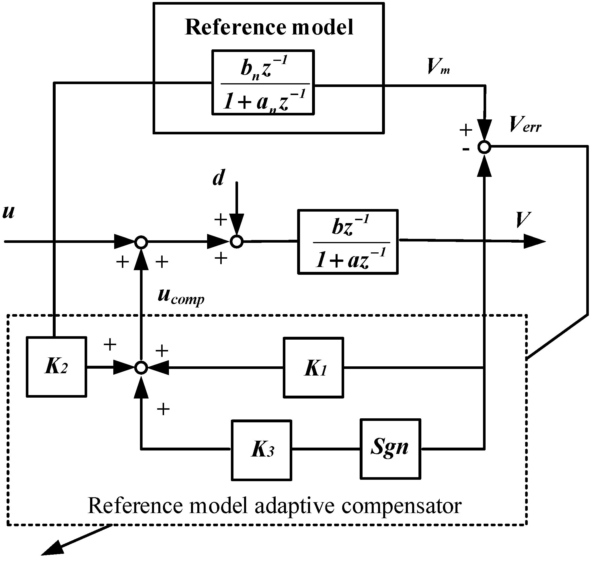
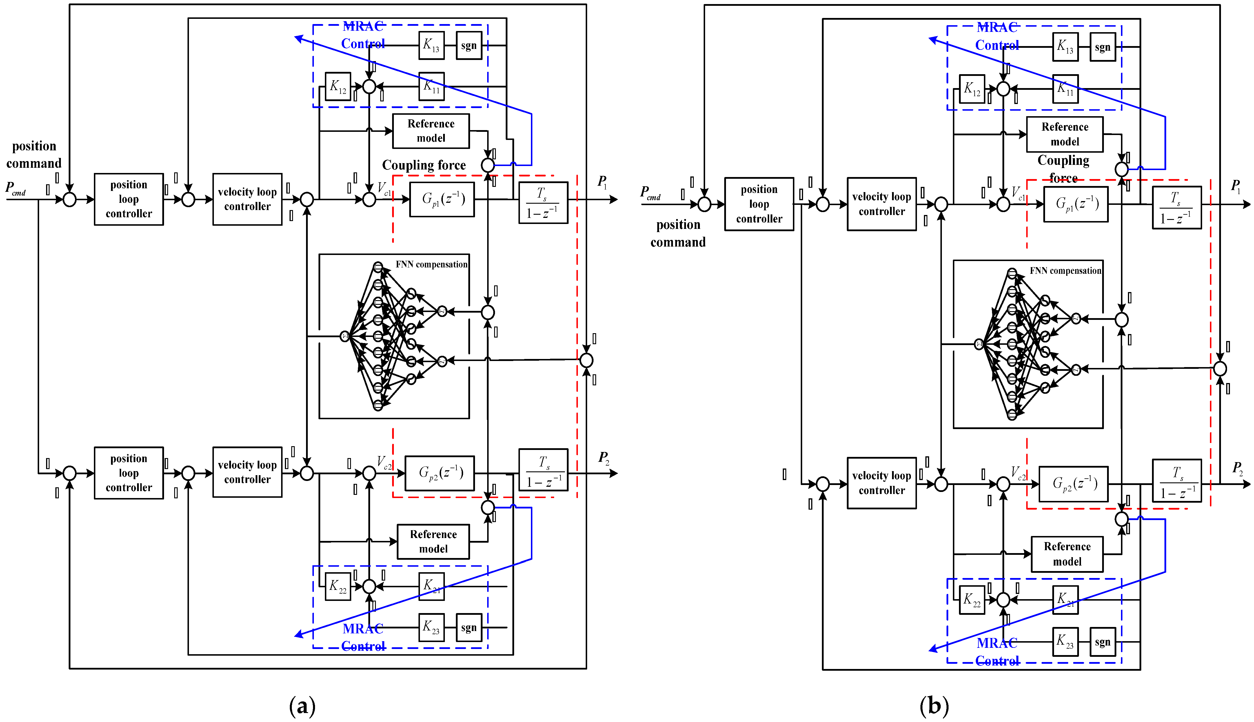
3. Proposed Control System

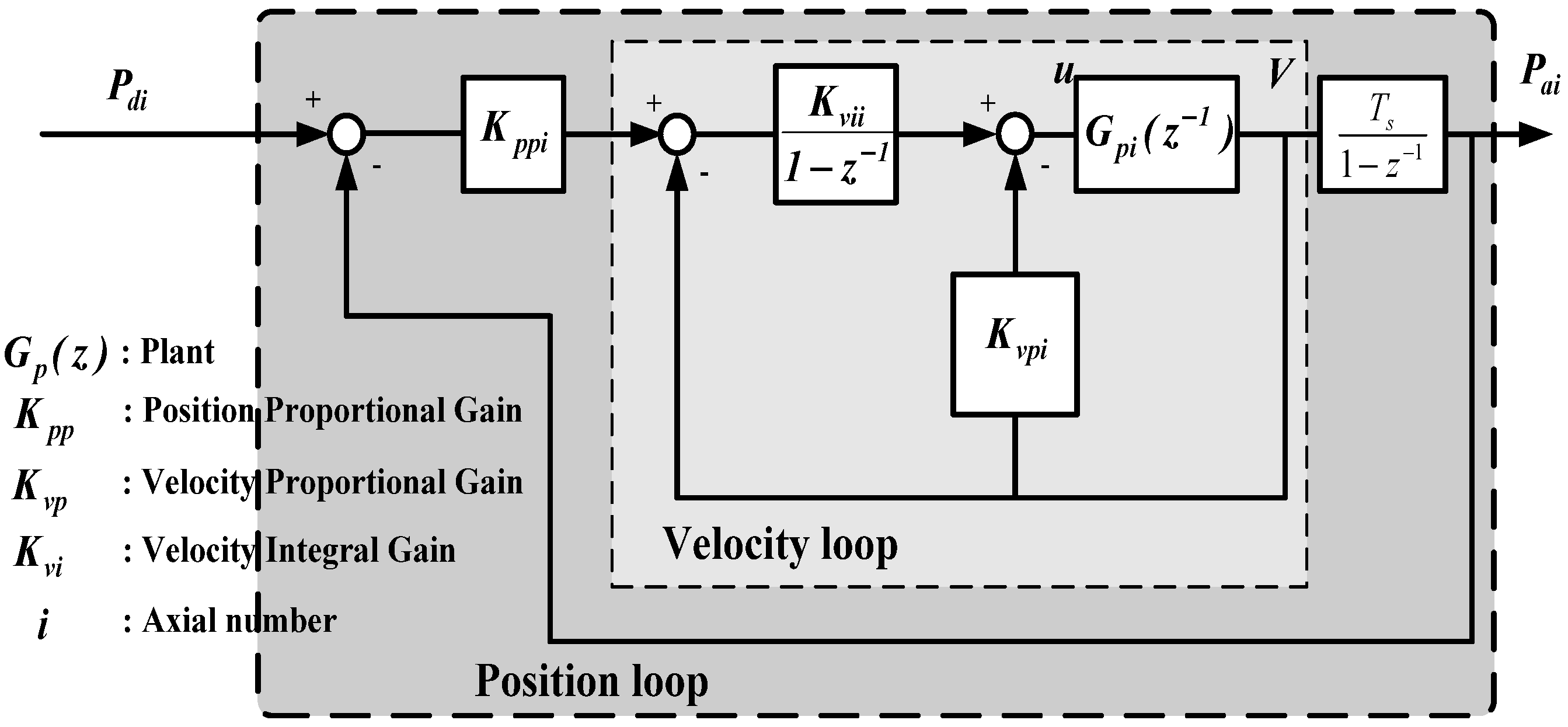
3.1. Controller Design for The Single Sxis

To reduce the tracking error of the single axis position, we adopt the cascade control method to design the single axis control, as shown in Figure 5. In this method, $G_{pi}\left(z^{-1}\right)$ is the discrete model of a single axis plant, which can be represented as

$$G_p\left(z^{-1}\right)=Z\left[\frac{1-e^{-Ts}}{s}\cdot \frac{K_i}{{\tau }_{i}s+1}\right]=\frac{b{z}^{-1}}{1+a{z}^{-1}}$$

(4)

where

$$\begin{gathered} a=-e^{-\raisebox{1ex}{$B\cdot Ts$}\!\left/ \!\raisebox{-1ex}{$J$}\right.} \\ b=\left(K_t/B\right)\left(1-e^{-\raisebox{1ex}{$B\cdot Ts$}\!\left/ \!\raisebox{-1ex}{$J$}\right.}\right) \end{gathered}$$

(5)

and $T_s$ is the sampling time.

The inner velocity loop and outer position loop use the integral K_vii, proportional K_vpi, and proportional K_ppi controllers. To make the reference model close to the real model, we adopted the adaptive control to let the reference model approach to real model. At present, there are two main design architectures in the adaptive control. One is the self-tuning controller (STC), and the other is the model reference adaptive controller (MRAC). Here, we adopted the MRAC [30], as shown in Figure 6. The basic concept of MRAC is to plan the performance of the control system in a reference model, and the design of the entire feedback control system is to match the planned reference model to achieve the expected system response.

From Figure 6, the adaptive force u_comp can be obtained by the error V_err, and the reference output V_m is composed of the nominal parameters a_n and b_n. The adaptive parameters K₁, K₂, and K₃ are derived from the Lyapunov stability criterion. The detailed derivation process, please see Appendix A.

$$\begin{gathered} K_1(N)=B_1{\displaystyle \sum _{i=0}^N{V}_{err}(i)\cdot V(i)+C_1\cdot V_{err}(N)\cdot V(N)} \\ {K}_2(N)=B_2{\displaystyle \sum _{i=0}^N{V}_{err}(i)\times u(i)+C_2\times V_{err}(N)\times u(N)} \\ {K}_3(N)=B_3{\displaystyle \sum _{i=0}^N{V}_{err}(i)\times \mathrm{sgn}(V(i))+C_3\times V_{err}(N)\times \mathrm{sgn}(V(i))} \end{gathered}$$

(6)

where the positive constants are $B_j$ and $C_j$, and j = 1, 2, 3, could be well tuned under the model reference adaptive control method. Therefore, the transfer function of the velocity inner loop can be represented as

$$T{F}_v(z)=\frac{K_{vpi}b{T}_{s}z}{z^2+(a-1+K_{vpi}b{T}_S+K_{vii}b{T}_s)z+(-a-K_{vii}b{T}_s)}$$

(7)

We can use the pole-placement method to design the controller for this second-order system. Let the two parameters $\xi$ and ${\omega }_n$ be similar to the damping ratio and natural frequency of the standard second-order system; then, the parameters of the velocity controller are

$$\begin{gathered} K_p=\frac{1+e^{-2\xi {\omega }_n{T}_s}-2e^{-\xi {\omega }_n{T}_S}\cos ({\omega }_d{T}_s)}{b{T}_s} \\ {K}_d=\frac{(e^{-2\xi {\omega }_n{T}_s}+a)}{-b} \end{gathered}$$

(8)

The transfer function of the outer position loop can be simplified as

$$\frac{P_{ai}}{P_{di}}=\frac{K_{ppi}{T}_s}{z+\left(K_{ppi}{T}_s-1\right)}$$

(9)

Here, the bandwidth of the position loop can be well designed according to the rule of cascade control, and then the parameter K_ppi can be easily obtained. For more details, please refer to [30]. Here, we adopt the important design results of [30].

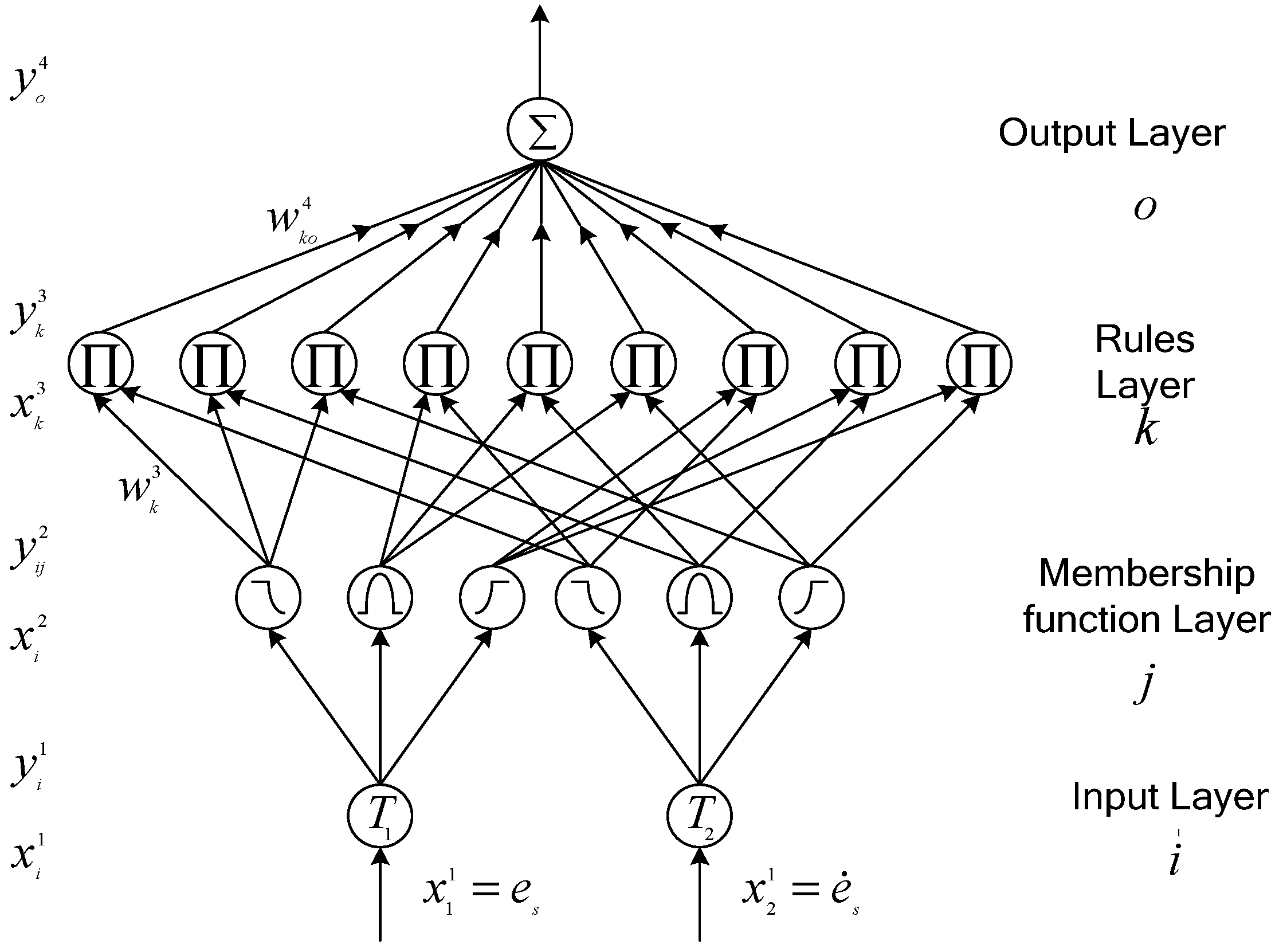
3.2. FNN Synchronous Motion Compensator

Although the abovementioned single axis controller can reduce the single axis position tracking error, the synchronous error between the dual motors is caused by various factors, such as unbalanced forces on both sides, various disturbances in the driving process and environmental uncertainty. This is an unavoidable situation. Therefore, we developed an FNN online compensator combined with MRAC, as shown in Figure 7. This FNN online compensator can compensate for the synchronous error online. Here, two methods are proposed: (1) parallel control and (2) parallel master–slave control. When the linear guides are not parallel with respect to each other axis in installation, the second method will be applied to avoid the mechanical coupling force being yielded by achieving the synchronous motion in position.

Adopting the concept of fuzzy neural network technology, the proposed FNN compensator for MRAC can be constructed, as shown in Figure 8.

Next, we introduce the important concepts of an FNN. An FNN is a network with fuzzy inference characteristics implemented by a four-layer neural network. The following will describe the structure, corresponding operation and learning process of an FNN.

Layer 1: Input layer

Each node in this layer represents the input node of each input linguistic variable and corresponds to an input variable. This means that the nodes in this layer are only responsible for passing the input signal to the next linguistic layer. There are two input variables of the FNN compensator in our proposed synchronous control method. One is the position synchronous error $x_1^1=e_s=P_1-P_2$, and the other is the velocity synchronous error $x_2^1={\dot{e}}_s=V_1-V_2$. P₁, P₂ are the position responses, and V₁ and V₂ are the velocity responses corresponding to Axes 1 and 2, respectively. Therefore, the node output of this layer is as follows:

$$y_i^1(N)=T_i\cdot x_i^1(N),i=1,2$$

(10)

Layer 2: Linguistic layer (Membership layer)

The nodes in layer 2 are called membership nodes, and the role of this layer is to perform the membership function of each node. The Gaussian function is used here as a membership function. Then,

$$y_{ij}^2(N)=\exp \left[-\frac{{(x_i^2-m_{ij})}^2}{{({\sigma }_{ij})}^2}\right],i=1,2;j=1,2,\dots ,M$$

(11)

where $m_{ij}$ and ${\sigma }_{ij}$ denote the mean and the standard deviation, respectively, of the Gaussian functions of the jth term of the ith input linguistic variable; M is the number of rules.

Layer 3: Rule layer

The rule nodes are located in layer 3, which includes the rule layer and fuzzy inference mechanism. For each layer 3 node, there is at most one previous link from the layer 2 node of the language variable. The nodes in this layer are denoted by $\prod$, which are multiplied by the input signal from layer 2. Then, for the jth rule node,

$$y_k^3(N)=\prod _{i=1}^2{w}_k^3\cdot y_{ij}^2(N)i=1,2j=1,2,\dots ,M$$

(12)

where $y_k^3$ and $w_k^3$ represent the output and weight of the rule layer, respectively. Here, $w_k^3$ is designed to be 1.

Layer 4: Output layer

The layer 4 contains output variable nodes. This layer performs defuzzification to obtain the numerical output $y_o^4$. The operation of layer 4 is

$$y_o^4(N)=\sum _k{w}_{ko}^4\cdot y_k^3$$

(13)

where $y_o^4(N)$ is the output of the proposed FNN compensator for MRAC and the link weight $w_{ko}^4$ is the output strength. In this paper, M is set to 3, which means that the linguistic layer has 6 nodes, and the rule layer has 9 nodes.

3.3. On-Line Learning Algorithm

The parameter learning algorithm is based on a supervised learning law to train the system. This method is the same as the derivation of the back propagation algorithm, adjusting the link weight in the output layer to minimize the given energy function.

$$E=\frac{1}{2}{e}_s{}^2+\frac{1}{2}{\dot{e}}_s{}^2$$

(14)

Next, we describe the update laws of the parameters in the FNN. First, the error term to be propagated is given by

$${\delta }_o^4=-\frac{\partial E}{\partial y_o^4}=-\frac{1}{2}\frac{\partial E}{\partial e_s}\frac{\partial e_s}{\partial y_o^4}-\frac{1}{2}\frac{\partial E}{\partial {\dot{e}}_s}\frac{\partial {\dot{e}}_s}{\partial y_o^4}=-\frac{1}{2}{e}_s\frac{\partial e_s}{\partial y_o^4}-\frac{1}{2}{\dot{e}}_s\frac{\partial {\dot{e}}_s}{\partial y_o^4}$$

(15)

The exact calculation of the Jacobian of systems $\partial e_s/\partial y_o^4$ and $\partial {\dot{e}}_s/\partial y_o^4$, which are contained in $\partial E/\partial y_o^4$, cannot be determined due to the uncertainties of the plant dynamics, such as parameter variations and external disturbances. To overcome this problem and to increase the online learning rate of the network parameters, the derivatives $\partial e_s/\partial y_o^4$ and $\partial {\dot{e}}_s/\partial y_o^4$ are approximated by the ratio of the signs of the changes in e_s and ${\dot{e}}_s$ with respect to $y_o^4$, respectively. In this study, the compensated force $y_o^4$ is used to reduce the synchronous errors of position e_s and velocity ${\dot{e}}_s$. Therefore,

$$\begin{gathered} \frac{\partial e_s}{\partial y_o^4}=sgn\left(\frac{\partial e_s}{\partial y_o^4}\right)=-1 \\ \frac{\partial {\dot{e}}_s}{\partial y_o^4}=sgn\left(\frac{\partial {\dot{e}}_s}{\partial y_o^4}\right)=-1 \end{gathered}$$

(16)

then, Equation (15) can be rewritten as

$${\delta }_o^4=-\frac{1}{2}{e}_s\frac{\partial e_s}{\partial y_o^4}-\frac{1}{2}{\dot{e}}_s\frac{\partial {\dot{e}}_s}{\partial y_o^4}=\frac{1}{2}\left(e_s+{\dot{e}}_s\right)$$

(17)

and the update of $w_{ko}^4$ is

$$\Delta w_{ko}^4=-{\eta }_w\frac{\partial E}{\partial w_{ko}^4}=\left[-{\eta }_w\frac{\partial E}{\partial y_o^4}\right]\left[\frac{\partial y_o^4}{\partial w_{ko}^4}\right]={\eta }_w{\delta }_o^4{y}_k^3$$

(18)

where ${\eta }_w$ is the learning rate parameter of the link weights. Then, the weights are updated as

$$w_{ko}^4(N+1)=w_{ko}^4(N)+\Delta w_{ko}^4$$

(19)

3.4. Stability Analysis

Refer to [31,32,33], based on the discrete Lyapunov function analysis, we consider the energy function (14) as the discrete Lyapunov function. The change in the Lyapunov function can be written as

$$\Delta V(N)=V(N+1)-V(N)$$

(20)

then, according to [31,32,33], Equation (20) will be derived as follows.

$$V(N+1)=V(N)+\Delta V(N)$$

$$\approx V(N)+{\displaystyle \sum _{j=1}^M\left[\frac{\partial V(N)}{\partial w_{ko}^4}\Delta w_{ko}^4\right]}+{\displaystyle \sum _{j=1}^M\left[\frac{\partial V(N)}{\partial w_k^3}\Delta w_k^3\right]}+{\displaystyle \sum _{j=1}^M{\displaystyle \sum _{i=1}^2\left[\frac{\partial V(N)}{\partial m_{ij}}\Delta m_{ij}+\frac{\partial V(N)}{\partial {\sigma }_{ij}}\Delta {\sigma }_{ij}\right]}}$$

(21)

By the design of the learning rate parameters [31], the convergence of Equation (21) can be guaranteed. Here, we have omitted some mathematical processes, and listed the important result as follows:

$$\begin{array}{l}V(N+1)\approx \epsilon ({\eta }_w+{\eta }_{\theta }+{\eta }_m+{\eta }_{\sigma })=\frac{V(N)\epsilon }{4\left[{\displaystyle \sum _{j=1}^M{((\partial V(N)/\partial y_o^4)(\partial y_o^4/\partial w_{ko}^4))}^2+\epsilon }\right]}+\frac{V(N)\epsilon }{4\left[{\displaystyle \sum _{j=1}^M{\displaystyle \sum _{i=1}^2{((\partial V(N)/\partial y_o^4)(\partial y_o^4/\partial w_k^3{y}_k^3)(\partial w_k^3{y}_k^3/\partial w_k^3))}^2+\epsilon }}\right]}+\\ \frac{V(N)\epsilon }{4\left[{\displaystyle \sum _{j=1}^M{\displaystyle \sum _{i=1}^2{((\partial V(N)/\partial y_o^4)(\partial y_o^4/\partial y_{ij}^2)(\partial y_{ij}^2/\partial m_{ij}))}^2+\epsilon }}\right]}+\frac{V(N)\epsilon }{4\left[{\displaystyle \sum _{j=1}^M{\displaystyle \sum _{i=1}^2{((\partial V(N)/\partial y_o^4)(\partial y_o^4/\partial y_{ij}^2)(\partial y_{ij}^2/\partial {\sigma }_{ij}))}^2+\epsilon }}\right]}\\ <\frac{V(N)}{4}+\frac{V(N)}{4}+\frac{V(N)}{4}+\frac{V(N)}{4}=V(N)\end{array}$$

(22)

From Equation (22), it means that the synchronous error of the gantry robot will gradually converge to zero.

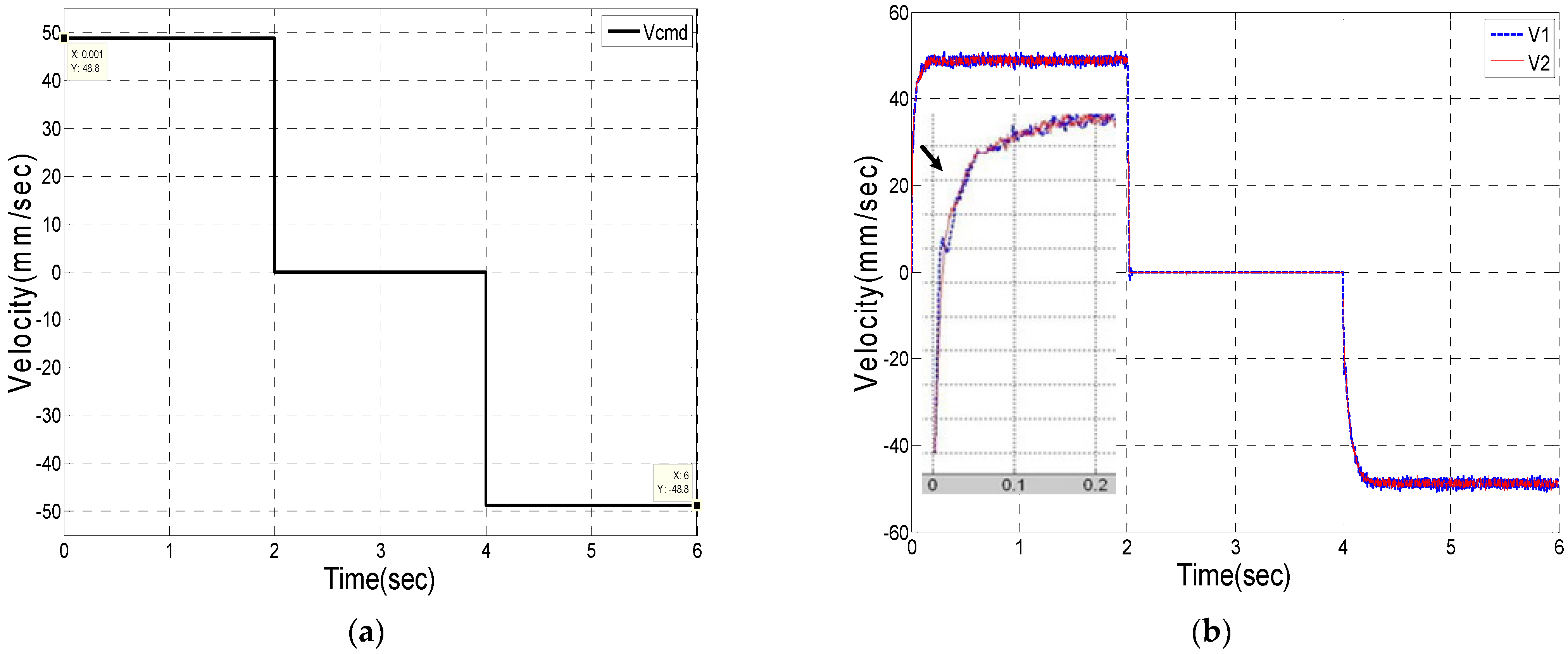
4. Experimental Results

Figure 9 shows the experimental system of the gantry robot control system in this study. In the experimental system, the single axis controller and the proposed FNN online compensator for MRAC are implemented in the PC.

In this study, a 1 msec sampling rate is adopted for the encoder interface and the execution of the control algorithm. For comparison, the results of experiments for low-frequency (1/5 Hz) and high-frequency (2/3 Hz) sinusoid position commands with the same strokes ($\pm$36.6 mm) are used to verify the synchronous control performance of cascade synchronous control, parallel synchronous control without a synchronous compensator and the proposed control methods in Figure 7. Here, we set the parameters of the proposed FNN compensator as $w_k^3=1$ and M = 3, which means that the linguistic layer has 6 nodes, and the rule layer has 9 nodes. Furthermore, the learning rate ${\eta }_w$ is designed to 0.001 to let the convergence of Equation (21) can be guaranteed. To provide an overall evaluation, two performance indices, the sum of absolute synchronous error and root mean square synchronous error, are defined as

$$\begin{gathered} E_{SAE}={\displaystyle \sum _{N_i}\left|e_s\right|} \\ {E}_{RMS}=\sqrt{\frac{1}{N_i}{{\displaystyle \sum _{N_i}\left(e_s\right)}}^2} \end{gathered}$$

(23)

Figure 10 shows the synchronous error of the cascade synchronous control method, shown in Figure 1a, by feeding the low-frequency command (1/5 Hz). The maximum synchronous error is approximately $\pm$0.92 mm even when the federate is low. In this method, the control efforts, depicted in Figure 11, indicate that they are not consistent in the phase and magnitude due to the servo lag between the master and slave axes and that the effect will yield a large synchronous error. Hence, this method is not suitable for gantry robot synchronous control. In the following discussion, the performance of the two proposed methods will be compared under different conditions: (1) without compensation; (2) with FNN compensation; and (3) with FNN and MRAC compensation.

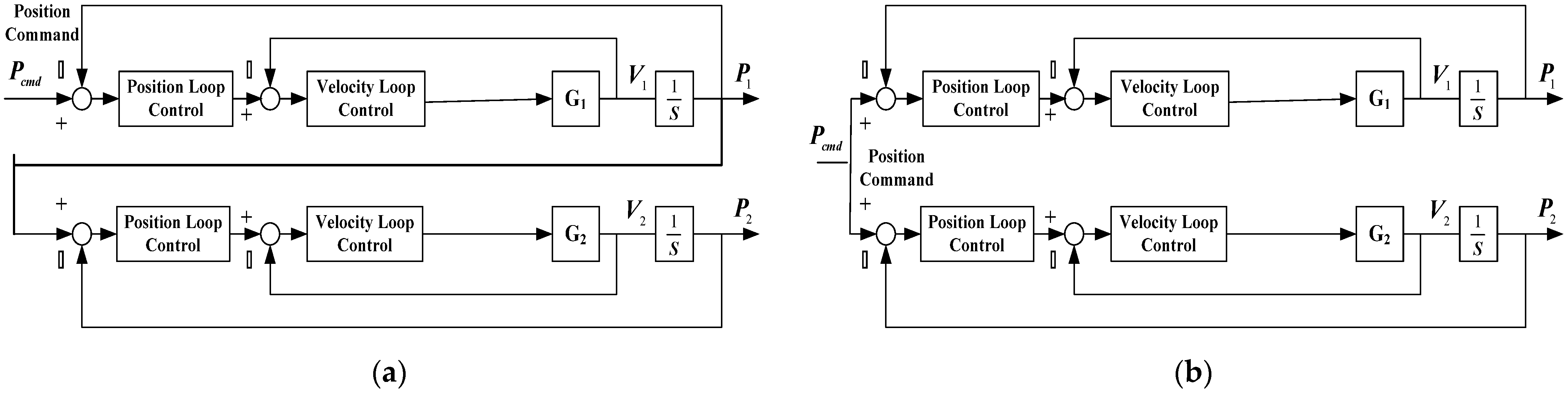
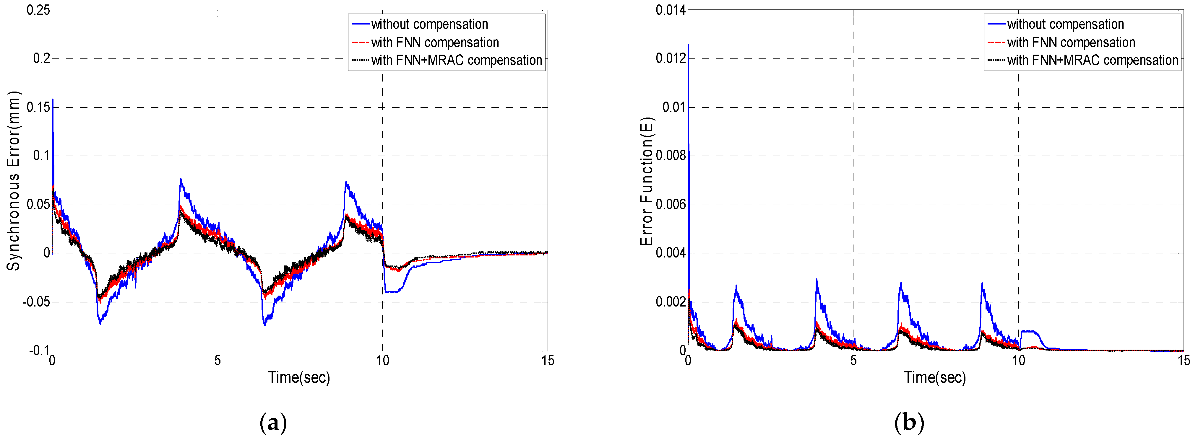
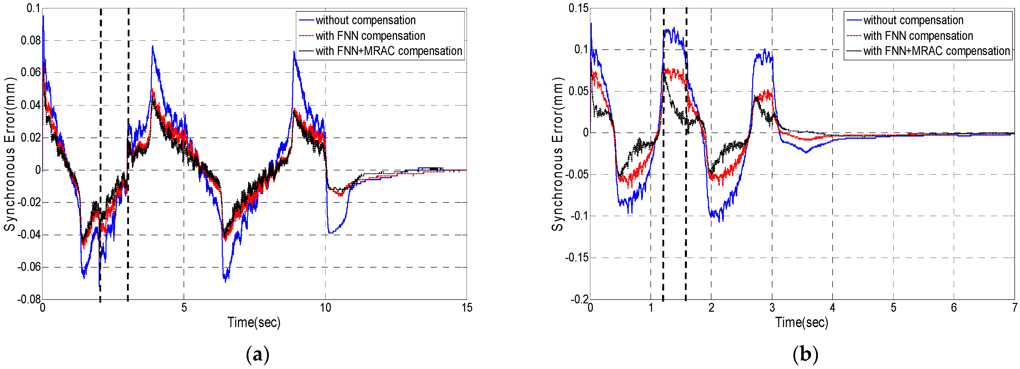
4.1. Parallel Synchronous Control

There are two kinds of position commands mentioned above fed to the parallel synchronous control method to test the synchronous performance. For low-frequency commands, the synchronous error and cost function shown in Equation (14) are depicted in Figure 12a,b. Figure 13a,b shows the case of a high-frequency command. When a constant disturbance 0.02375 N-m is applied to Axis 2 during the period of 2 to 3 s and 1.2 to 1.6 s corresponding to low- and high-frequency commands, respectively, and the synchronous errors will be magnified without a compensator. Figure 14a,b shows the synchronous errors with respect to low- and high-frequency commands. In contrast, these figures also show that the synchronous errors will be suppressed to be similar to the condition without disturbances by synchronous compensators. The detailed results of the two performance indices in Equation (20) are shown in

Table 2. Synchronous performance under low-frequency commands.

	Performance Index (mm)	No Compensation	FNN	FNN + MRAC
without disturbances	$E_{SAE}$	294.204	195.394	157.399
	$E_{RMS}$	0.0359	0.0235	0.0198
with disturbances	$E_{SAE}$	30.125	25.126	23.142
	$E_{RMS}$	0.0387	0.0241	0.0204

and

Table 3. Synchronous performance under low-frequency commands.

	Performance Index (mm)	No Compensation	FNN	FNN + MRAC
without disturbances	$E_{SAE}$	578.168	357.550	307.116
	$E_{RMS}$	0.0606	0.0383	0.0330
with disturbances	$E_{SAE}$	91.225	71.114	63.453
	$E_{RMS}$	0.0918	0.0709	0.0644

. The sampling points between the dotted lines shown in Figure 14a,b, where disturbances are applied, are calculated in the case of “with disturbances”.

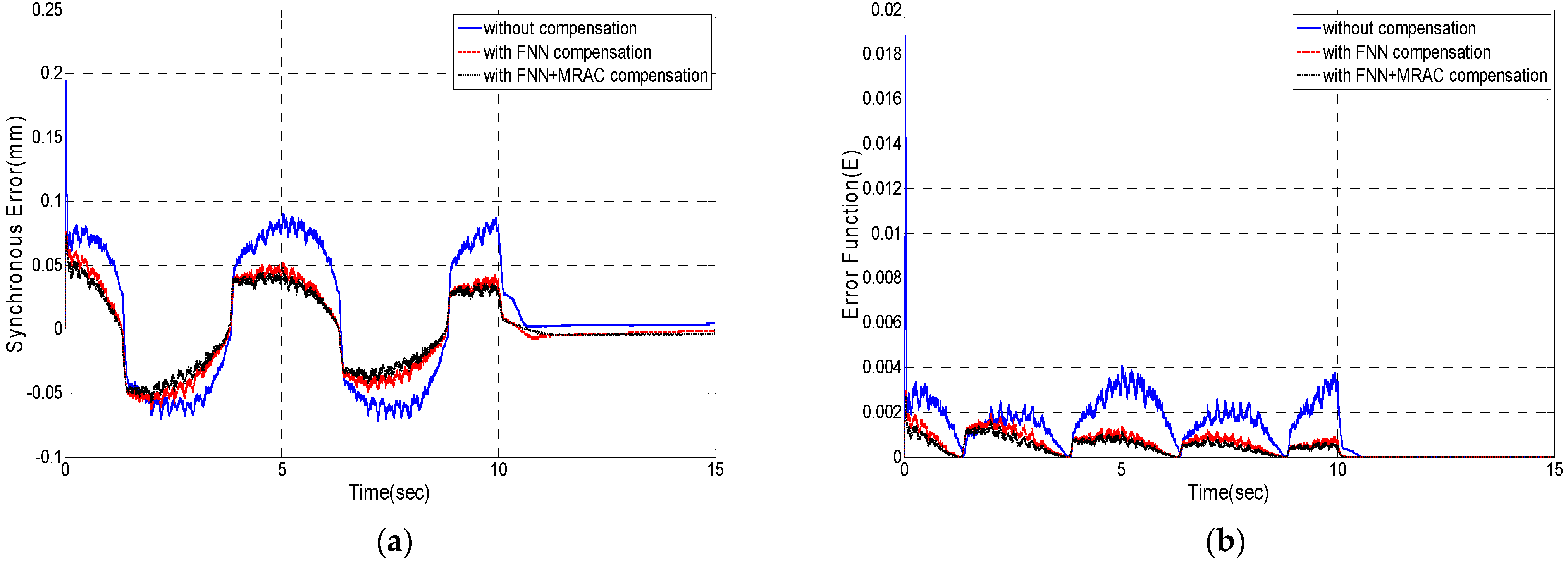
4.2. Parallel Master–Slave Synchronous Control

There are also two kinds of position commands mentioned above fed to the parallel master–slave synchronous control method to test the synchronous performance. For low-frequency commands, the synchronous error and cost function shown in Equation (14) are depicted in Figure 15a,b. Figure 16a,b shows the case of a high-frequency command. When a constant disturbance 0.02375 N-m is applied to Axis 2 during 2 to 3 s and 1.2 to 1.6 s corresponding to low- and high-frequency commands, respectively, and the synchronous errors will be magnified without a compensator. Figure 17a,b shows the synchronous errors with respect to low- and high-frequency commands. In contrast, these figures also show that the synchronous errors will be suppressed to be similar to the condition without disturbances by synchronous compensators. The detailed results of the two performance indices in Equation (23) are shown in

Table 4. Synchronous performance under high-frequency commands.

	Performance Index (mm)	No Compensation	FNN	FNN + MRAC
without disturbances	$E_{SAE}$	208.891	124.671	71.494
	$E_{RMS}$	0.0768	0.0461	0.0278
with disturbances	$E_{SAE}$	48.253	29.221	15.223
	$E_{RMS}$	0.117	0.0653	0.0341

and

Table 5. Synchronous performance under high-frequency commands.

	Performance Index (mm)	No Compensation	FNN	FNN + MRAC
without disturbances	$E_{SAE}$	262.844	189.101	129.021
	$E_{RMS}$	0.0914	0.0667	0.0449
with disturbances	$E_{SAE}$	52.573	35.891	26.432
	$E_{RMS}$	0.129	0.0892	0.0654

. The sampling points between the dotted lines shown in Figure 17a,b, where the disturbances are applied, are calculated in the case of “with disturbances”.

In addition, we use the parameter settings of [34] to realize the performance of the PID compensator, as shown in Figure 18. The synchronous errors under different control schemes are shown in

Table 6. Synchronous performance under different control schemes.

Performance Index (mm)	No Compensation	FNN	FNN + MRAC
$E_{RMS}$	0.04	0.024	0.02

.

5. Conclusions

This paper has proposed MRAC controllers and FNN online compensators for a gantry robot. We successfully completed the theoretical and technical feasibility of the proposed method through various experimental comparisons. From Table 2, Table 3, Table 4 and Table 5, we demonstrate the advantages of our proposed method (FNN + MRAC) for the synchronous errors and the design can enhance robustness to uncertainty. In addition, this study also successfully integrates the hardware and successfully verifies the proposed methods. For the future research direction, because this paper does not analyze and deal with the influence of friction, the analysis and compensation of friction will be the future development direction.

References

1. Luo, R.C.; Perng, Y.W. Adaptive skew force free model-based synchronous control and tool center point calibration for a hybrid 6-DoF gantry-robot machine. IEEE/ASME Trans. Mechatron. 2020, 25, 964–976. [Google Scholar] [CrossRef]
2. Tan, K.K.; Lee, T.H.; Huang, S. Precision Motion Control; Springer: Berlin/Heidelberg, Germany, 2008. [Google Scholar]
3. Li, C.; Li, C.; Chen, Z.; Yao, B. Advanced synchronization control of a dual-linear-motor-driven gantry with rotational dynamics. IEEE Trans. Ind. Electron. 2018, 65, 7526–7535. [Google Scholar] [CrossRef]
4. Koren, Y. Cross-coupled biaxial computer control for manufacture systems. ASME J. Dyn. Syst. Meas. Control 1980, 102, 265–272. [Google Scholar] [CrossRef]
5. Giam, T.S.; Tan, K.K.; Huang, S. Precision coordinated control of multi-axis gantry stages. ISA Trans. 2007, 46, 399–409. [Google Scholar] [CrossRef] [PubMed]
6. Lu, L.; Chen, Z.; Yao, B.; Wang, Q. Desired compensation adaptive robust control of a linear-motor-driven precision industrial gantry with improved cogging force compensation. IEEE/AMSE Trans. Mechatron. 2008, 13, 617–624. [Google Scholar] [CrossRef]
7. Chen, S.L.; Lin, W.M.; Chang, T.H. Tracking control for a synchronized dual parallel linear motor machine tool. Proc. Inst. Mech. Eng. Part I: J. Syst. Control Eng. 2008, 222, 851–862. [Google Scholar] [CrossRef]
8. Tsai, W.C.; Wu, C.H.; Cheng, M.Y. Tracking accuracy improvement based on adaptive nonlinear sliding mode control. IEEE/ASME Trans. Mechatron. 2021, 26, 179–190. [Google Scholar] [CrossRef]
9. Zhao, J.; Mou, Q.; Zhu, C.; Chen, Z.; Li, J. Study on a double-sided permanent-magnet linear synchronous motor with reversed slots. IEEE/AMSE Trans. Mechatron. 2021, 26, 3–12. [Google Scholar] [CrossRef]
10. Wu, X.; She, J.; Yu, L.; Dong, H.; Zhang, W.A. Contour tracking control of networked motion control system using improved equivalent-input-disturbance approach. IEEE Trans. Ind. Electron. 2021, 68, 5155–5165. [Google Scholar] [CrossRef]
11. Chen, C.S.; Fan, Y.H.; Tseng, S. Position command shaping control in a retrofitted milling machine. Int. J. Mach. Tools Manuf. 2006, 46, 293–303. [Google Scholar] [CrossRef]
12. Sun, D. Position synchronization of multiple motion axes with adaptive coupling control. Automatica 2003, 39, 997–1005. [Google Scholar] [CrossRef]
13. Wang, Y.W.; Zhang, W.A.; Yu, L. GESO-based position synchronization control of networked multiaxis motion system. IEEE Trans. Ind. Inform. 2020, 16, 248–257. [Google Scholar] [CrossRef]
14. Chen, Z.; Li, C.; Yao, B.; Yuan, M.; Yang, C. Integrated coordinated/synchronized contouring control of a dual-linear-motor-driven gantry. IEEE Trans. Ind. Electron. 2020, 67, 3944–3954. [Google Scholar] [CrossRef]
15. Hu, C.; Yao, B.; Wang, Q. Coordinated adaptive robust contouring controller design for an industrial biaxial precision gantry. IEEE/ASME Trans. Mechatron. 2010, 15, 728–735. [Google Scholar]
16. Yemelyanov, V.; Chernyi, S.; Yemelyanova, N.; Varadarajan, V. Application of neural networks to forecast changes in the technical condition of critical production facilities. Comput. Electr. Eng. 2021, 93, 107225. [Google Scholar] [CrossRef]
17. Demby’s, J.; Gao, Y.; DeSouza, G.N. A Study on solving the inverse kinematics of serial robots using artificial neural network and fuzzy neural network. In Proceedings of the 2019 IEEE International Conference on Fuzzy Systems (FUZZ-IEEE), New Orleans, LA, USA, 23–26 June 2019; pp. 1–6. [Google Scholar]
18. Chetyrbok, P.V. Fuzzy neural networks for classification of problems. In Proceedings of the 2021 XXIV International Conference on Soft Computing and Measurements (SCM), St. Petersburg, Russia, 26–28 May 2021; pp. 133–135. [Google Scholar]
19. Wang, L.X. A Course in Fuzzy Systems and Control; Prentice-Hall Press: Hoboken, NJ, USA, 1997. [Google Scholar]
20. Xiao, L.; Zhang, Z.; Li, S. Solving time-varying system of nonlinear equations by finite-time recurrent neural networks with application to motion tracking of robot manipulators. IEEE Trans. Syst. Man Cybern. Syst. 2019, 49, 2210–2220. [Google Scholar] [CrossRef]
21. Wan, P.; Sun, D.; Zhao, M.; Huang, S. Multistability for almost-periodic solutions of Takagi–Sugeno fuzzy neural networks with nonmonotonic discontinuous activation functions and time-varying delays. IEEE Trans. Fuzzy Syst. 2021, 29, 400–414. [Google Scholar] [CrossRef]
22. Lin, C.J.; Chin, C.C. Prediction and identification using wavelet-based recurrent fuzzy neural networks. IEEE Trans. Syst. Man Cybern. Part B Cybern. 2004, 34, 2144–2154. [Google Scholar] [CrossRef]
23. Wang, J.; Luo, W.; Liu, J.; Wu, L. Adaptive type-2 FNN-based dynamic sliding mode control of DC–DC boost converters. IEEE Trans. Syst. Man Cybern. Syst. 2021, 51, 2246–2257. [Google Scholar] [CrossRef]
24. Han, M.; Zhong, K.; Qiu, T.; Han, B. Interval Type-2 fuzzy neural networks for chaotic time series prediction: A concise overview. IEEE Trans. Cybern. 2019, 49, 2720–2731. [Google Scholar] [CrossRef]
25. Na, J.; Wang, S.; Liu, Y.J.; Huang, Y.; Ren, X. Finite-time convergence adaptive neural network control for nonlinear servo systems. IEEE Trans. Cybern. 2020, 50, 2568–2579. [Google Scholar] [CrossRef] [PubMed]
26. Kayacan, E.; Kayacan, E.; Ramon, H.; Saeys, W. Adaptive neuro- fuzzy control of a spherical rolling robot using sliding-mode-control- theory-based online learning algorithm. IEEE Trans. Cybern. 2013, 43, 170–179. [Google Scholar] [CrossRef]
27. Dou, H.; Lu, H.; Wang, S.; Liu, Q.; Wang, D.; Meng, L. Research on synchronous control of gantry-type dual-driving feed system based on fuzzy single neuron PID cross-coupled controller. In Proceedings of the IEEE 5th Advanced Information Technology, Electronic and Automation Control Conference (IAEAC), Chongqing, China, 12–14 March 2021; pp. 1107–1112. [Google Scholar]
28. Jung, H.; Oh, S. Disturbance observer based decoupling control to suppress rotational motion of cross-coupled gantry stage. In Proceedings of the IEEE 28th International Symposium on Industrial Electronics (ISIE), Vancouver, BC, Canada, 12–14 June 2019; pp. 503–508. [Google Scholar]
29. Chen, C.S.; Chen, S.K.; Chen, L.Y. Disturbance observer-based modeling and parameter identification for synchronous dual-drive ball screw gantry stage. IEEE ASME Trans. Mechatron. 2019, 24, 2839–2849. [Google Scholar] [CrossRef]
30. Gilbart, J.W.; Winston, G.C. Adaptive compensation for an optical tracking telescope. Automatica 1974, 10, 125–131. [Google Scholar] [CrossRef]
31. Chou, P.H.; Chen, C.S.; Lin, F.J. DSP-based synchronous control of dual linear motors via Sugeno type fuzzy neural network compensator. J. Franklin Inst. 2012, 349, 792–812. [Google Scholar] [CrossRef]
32. Tan, K.H.; Lin, F.J.; Chen, J.H. DC-link voltage regulation using RPFNN-AMF for three-phase active power filter. IEEE Access 2018, 6, 37454–37463. [Google Scholar] [CrossRef]
33. Yoo, S.J.; Choi, Y.H.; Park, J.B. Generalized predictive control based on self-recurrent wavelet neural network for stable path tracking of mobile robots: Adaptive learning rates approach. IEEE Trans. Circuits Syst. 2006, 53, 1381–1395. [Google Scholar]
34. Wu, K.Z. Iterative Learning Command Shaping and Cross-Coupled PIDNN Synchronous Controller for H-Type Gantry Stage. Master’s Thesis, National Taipei University of Technology, Taipei, Taiwan, 2014. [Google Scholar]
35. Yang, T.H. Fuzzy Neural Network Synchronous Control of Gantry Stage. Master’s Thesis, National Taipei University of Technology, Taipei, Taiwan, 2011. [Google Scholar]
Figure 1. Typical methods to synchronize the motion in gantry robots: (a) cascade control method; (b) parallel control method.
Energies 15 00123 g001
Figure 2. The hardware structure of the gantry robot.
Energies 15 00123 g002
Figure 3. The PI controller loop for parameter identification.
Energies 15 00123 g003
Figure 4. (a) Velocity command; (b) velocity response.
Energies 15 00123 g004
Figure 5. Position loop control of single axis.
Energies 15 00123 g005
Figure 6. The model reference adaptive control method for the single axis system.
Energies 15 00123 g006
Figure 7. The proposed synchronous control methods of the gantry robot: (a) parallel control method; (b) parallel master–slave control method.
Energies 15 00123 g007
Figure 8. The proposed FNN compensator for MRAC.
Energies 15 00123 g008
Figure 9. The hardware setup of the PC-based control system in the gantry robot.
Energies 15 00123 g009
Figure 10. The synchronous error of the cascade synchronous control method.
Energies 15 00123 g010
Figure 11. Control efforts of the cascade synchronous control method.
Energies 15 00123 g011
Figure 12. (a) The synchronous error under low-frequency commands; (b) the cost function under low-frequency commands.
Energies 15 00123 g012
Figure 13. (a) The synchronous error under high-frequency commands; (b) the cost function under high-frequency commands.
Energies 15 00123 g013
Figure 14. (a) The synchronous error under low-frequency commands with disturbances. (b) the synchronous error under high-frequency commands with disturbances.
Energies 15 00123 g014
Figure 15. (a) The synchronous error under low-frequency commands; (b) the cost function under low-frequency commands.
Energies 15 00123 g015
Figure 16. (a) The synchronous error under high-frequency commands; (b) the cost function under high-frequency commands.
Energies 15 00123 g016
Figure 17. (a) The synchronous error under low-frequency commands with disturbances; (b) the synchronous error under high-frequency commands with disturbances.
Energies 15 00123 g017
Figure 18. The performance of the PID compensator: (a) the tracking error of Axis 1; (b) the tracking error of Axis 2; (c) the synchronous error.
Energies 15 00123 g018