Price Leadership and Volatility Linkages between Oil and Renewable Energy Firms during the COVID-19 Pandemic

Abstract

The COVID-19 pandemic is having a strong influence in all areas of society, like wealth, economy, travel, lifestyle habits, and, amongst many others, financial and energy markets. The influence in standard energies, like crude oil, and renewable energies markets has been twofold: from one side, the predictability of volatility has strongly decreased; secondly, the linkages of the price time series have been modified. In this paper, by using DCC-GARCH and Price Leadership Share methodology, we can investigate the changes in the influences between standard energies and renewable energies markets by analyzing one-minute time series of West Texas Intermediate crude oil futures contract (WTI), the Brent crude oil futures contract (BRENT), the STOXX Europe 600 oil & gas index (SXEV), and the European renewable energy index (ERIX). Our results confirm volatility spillover between the time series. However, when assessing the accuracy of the predictability of the DCC-GARCH model, the results show that the model fails its prediction in the period of higher instability. Besides, we found that price leadership has been strongly influenced by the virus spreading stages. These results have been obtained by dividing the period between September 2019 and January 2021 into 6 subperiods according to the pandemic stages.

1. Introduction

The COVID-19 pandemic has had, and still has, a strong influence in all areas of society, like wealth, economy, travel, lifestyle habits, and, amongst many others, financial markets. Many authors have already studied the consequences of the COVID-19 pandemic on financial systems. For instance, in Reference [1], the author notes several possible long-term adjustments to financial systems caused by COVID-19. In our paper, we focus the attention on the oil market, which experienced, for the first time, a negative spike in the price of the West Texas Intermediate (WTI) crude oil futures contract in April 2020 due to declining global demand. As reported in Reference [2], the crude oil market experienced strong price fluctuations in the period between March and April 2020 due to the price war between Russia and Saudi Arabia. The authors assessed the predictive power of historical uncertainty related to infectious diseases, not only COVID-19, for oil return volatility. Other authors tried to assess the influence of the extreme conditions we are experiencing on co-movements and spillovers of oil and renewable firms [3]. They focused their attention on the period of April 2020, where WTI oil future prices became negative.

In this paper, we study the influence of the COVID-19 outbreak on two crude oil futures contracts, the West Texas Intermediate (WTI) and the Brent crude oil (BRENT), and two market indexes, namely the STOXX Europe 600 oil & gas index (SXEV) and the European renewable energy index (ERIX). We employ a multivariate GARCH model, the DCC-GARCH model, to study the volatility spillover between the four mentioned stocks. Historically, ARCH models, introduced by Reference [4], have been a popular choice to model financial univariate time series with time-varying volatility. These models are Markovian stochastic processes with zero mean and non-constant time-dependent variances. Such models have global stationarity and local non-stationary behavior [5,6,7,8,9]. A generalization of ARCH models are GARCH models introduced by Reference [10]. GARCH models are simple models which have the advantage of easy estimation of the parameters. Even in their simplest forms, this family of models has proven surprisingly successful in predicting conditional variances [6,11,12,13,14]. The predictability of the time series of financial returns using GARCH models have been explored in Reference [15]. To allow volatility linkages between the time series and to generalize to multivariate models, Engle [16] introduced the DCC-GARCH model. This model has been extensively applied to financial markets, in particular to the oil market. For example, some authors analyze the volatility interactions between the oil market and the foreign exchange market [17,18] while others study the linkages between the oil market and the stock indices [19]. Moreover, the DCC-GARCH model has been used to study the volatility spillover between fuel oil and stock index futures markets in China by considering its time-variant feature [20] and to test the existence of financial contagion during the U.S. subprime crisis [21]. While extensions and variations of the multivariate GARCH models have been extensively studied in the past years, see, for example, Reference [22], the DCC-GARCH model remains an easy model to implement, and it is widely used also by practitioners.

The epidemic spread of COVID-19 in 2020 has given rise to a worldwide financial crisis during which the oil price has reached negative values for the first time. The DCC-GARCH model has already proven to be a useful tool to model volatility in financial crises [21]. Therefore, we apply it to the four mentioned indexes, WTI, BRENT, SXEV, and ERIX, to analyze the effect of the COVID-19 on their volatility prediction. To this extent, we study the period from September 2019 until January 2021 and divide it into six subperiods according to different stages of the virus spreading.

Moreover, we investigate the potential variability of the price leadership as a consequence of the COVID-19 spread. To this end, we applied a multivariate Markov model by implementing the Mixture Transition Distribution model (MTD) to analyze the time series of returns. The multivariate Markov model, introduced by Reference [23] for categorical data, has been recently implemented in the analysis of financial time series. D’Amico and De Blasis [24] proposed a multivariate stochastic dividend discount model based on the MTD model, while De Blasis [25] applied the same model to the analysis of price discovery in financial markets. MTD model by Reference [26] is mainly used to reduce the number of parameters to obtain a more parsimonious model. We used MTD to investigate the price leadership amongst the four indices in the six periods related to virus spreading.

Then, the contribution of the paper is twofold: from one side, we investigate the performance of DCC-GARCH in predicting the volatility during financial crises and, for the first time, during a period of negative oil prices; the second contribution is given by the use of price leadership share to assess the effect of the pandemic spread to the linkages between the series in terms of prices.

The paper is organized as follows: in Section 2, we give descriptive statistics of the database used in this work and a description of the DCC-GARCH model and Price Leadership methodology. In Section 3, we show the results obtained by the application of the two models, followed by some discussion in Section 4. Finally, we give conclusions and some outlooks.

2. Data and Methodology

2.1. Data

The data for the analysis are collected from the Thomson Reuters Refinitiv Datascope database. The sample includes two different price series for crude oil, i.e., the West Texas Intermediate crude oil futures contract (WTI) and the Brent crude oil futures contract (BRENT), and two market indexes, namely the STOXX Europe 600 oil & gas index (SXEV) and the European renewable energy index (ERIX). The WTI futures contract is traded on the New York Mercanticle Exchange (NYMEX), and it is often considered a benchmark in oil pricing along with the Brent crude oil, which refers to the oil extracted from the North Sea of Northwest Europe and whose futures contracts are traded on the Intercontinental Exchange (ICE). Both futures contracts are traded in U.S. dollars, and their full price series are created through the Thomson Reuters rolling feature, which uses, for each month, the active contract that is closer to maturity.

On the stock market side, we selected two indexes that are related to the energy market and which can affect and be affected by the oil market. The STOXX Europe 600 oil & gas index (SXEV) is a market capitalization weighted index comprising the top 20 European companies operating in the oil & gas sector, e.g., Total, Royal Dutch Shell, BP and others. It includes also a few companies operating in the renewable energy sector. However, their weight within the index is only around 10%. Thus, we can consider the SXEV index as strictly related to the oil market. On the contrary, the European renewable energy index (ERIX) tracks the performance of European companies operating in the following areas: biofuels, geothermal, marine, solar, water, and wind. Similarly to the SXEV index, the weighting scheme of the ERIX index is based on the companies’ market capitalization. Both indexes series are total return indexes and retrieved in U.S. dollars to make their prices comparable to the crude oil ones.

The sample period is from 1 September 2019 to 31 December 2020 to include a reference period before the COVID-19 pandemic spread. The sample includes transactions data sampled at 1-min frequency between 8:00 a.m. and 4:50 p.m. London time. The day time range is chosen according to the availability of the index data which coincides with the opening hours of the main European stock markets, during which all four time series are open for trading. It is worth to mention that the WTI futures contract operates on a 23 h basis. Therefore, the selection of the sample is not affected by the U.S. market closures. Weekends, holidays, and half trading days in any of the considered markets are excluded from the sample.

To visualize and understand the effect of the the COVID-19 pandemic, we divide the full period of analysis into subperiods following the main reported pandemic events made available by The Guardian [27] and the American Journal of Managed Care website [28]. Therefore, we define six subperiods, with the first one just before the COVID-19 pandemic, up to 31 December 2019, and the others distributed over the year 2020. We identify an initial Chinese spread at the beginning of the year up to the WHO’s declaration of the world pandemic, followed by a worldwide spread lasting up to the beginning of the summer. Then, a summer reopening period which faced a more relaxed atmosphere almost everywhere in Europe. Starting with the autumn, we can identify a second spread of the virus and, finally, the vaccine period with the announcement of the Pfizer results.

Figure 1 shows the four price series for the selected period split by subperiods. It is evident that prices started dropping as soon as the news of the new Chinese virus started spreading all over the world, with the exception of the ERIX index. Moreover, with the worldwide explosion of the COVID-19 pandemic around March and April 2020, after the WHO’s declaration of the world pandemic on 11 March 2020. All prices faced a relevant drop. In particular, the WTI prices became negative on 21 April 2020. Besides, both oil prices, as well as the oil & gas index (SXEV), were not able to fully recover the previous price levels. They faced a quite stable summer reopening, followed by other smaller plunges during the second pandemic wave in autumn 2020. Nonetheless, it is important to notice that the renewable index (ERIX) kept its upward trend, with some instability around the announcement of the pandemic and during the second spread, while the entire oil market struggled.

For a better understanding of the oil and renewable energy markets during the COVID-19 pandemic, in

Table 1. Summary statistics of the 1-min percentage returns for the four contracts from 1 September 2019 to 31 December 2020, time range from 8:00 a.m. to 4:50 p.m. London time. The four contracts are the West Texas Intermediate crude oil futures contract (WTI), the Brent crude oil futures contract (BRENT), the STOXX Europe 600 oil & gas index (SXEV), and the European renewable energy index (ERIX).

		WTI	BRENT	SXEV	ERIX
Period
Full dataset Obs: 172250	mean	−0.0001	−0.0001	−0.0001	0.0002
	std	0.5167	0.0964	0.0752	0.0604
	min	−102.0825	−7.5968	−4.4378	−3.7572
	max	83.2909	9.2275	2.4850	2.7950
	skew	−42.5313	2.8789	−2.0482	−1.2964
	kurt	18,424.3171	779.9667	179.6896	170.1605
Before COVID-19 Obs: 41870 01/09/2019–31/12/2019	mean	0.0001	0.0002	0.0001	0.0000
	std	0.0545	0.0533	0.0335	0.0385
	min	−1.3276	−1.3291	−0.3874	−1.8567
	max	0.9375	0.8087	0.4583	1.5288
	skew	−0.7698	−0.9137	−0.0603	−1.5519
	kurt	32.8249	30.1682	11.4476	282.9432
Chinese spread Obs: 24910 01/01/2020–10/03/2020	mean	−0.0007	−0.0007	−0.0016	0.0002
	std	0.0845	0.0804	0.0725	0.0555
	min	−1.0919	−1.4157	−4.4378	−2.3398
	max	1.8138	1.6868	1.5918	1.4196
	skew	0.5385	−0.0268	−20.5752	−3.3521
	kurt	29.3838	31.0702	1204.6331	199.2002
Worldwide spread Obs: 38690 11/03/2020–25/06/2020	mean	−0.0007	−0.0007	0.0000	−0.0005
	std	1.0833	0.1673	0.1187	0.0876
	min	−102.0825	−7.5968	−1.5095	−1.5770
	max	83.2909	9.2275	2.4850	1.5260
	skew	−20.5485	2.5072	0.6524	−0.0496
	kurt	4244.3328	379.5144	18.5669	21.1941
Summer reopening Obs: 31800 26/06/2020–21/09/2020	mean	0.0001	0.0000	−0.0004	0.0005
	std	0.0622	0.0563	0.0584	0.0481
	min	−0.8001	−0.6795	−0.5547	−0.6053
	max	1.0206	0.4540	0.4982	0.5568
	skew	0.0066	−0.0971	−0.0057	−0.0422
	kurt	8.1460	4.6936	4.5363	9.3955
Second spread Obs: 17490 22/09/2020–08/11/2020	mean	0.0003	0.0002	0.0001	0.0010
	std	0.0726	0.0676	0.0645	0.0611
	min	−0.8661	−0.7144	−0.8050	−3.7572
	max	0.6104	0.4884	0.9364	1.1464
	skew	−0.1302	−0.0582	0.2196	−12.7377
	kurt	6.9856	4.3737	7.9225	830.9181
Vaccines Obs: 17490 09/11/2020–31/12/2020	mean	0.0009	0.0009	0.0016	0.0006
	std	0.0637	0.0573	0.0634	0.0555
	min	−2.7700	−1.0395	−0.5734	−0.6306
	max	0.7251	0.6735	0.9992	2.7950
	skew	−4.6746	−0.3737	0.4145	7.1639
	kurt	213.7327	15.1881	11.2031	374.2154

, we report the summary statistics of the 1-min percentage returns for the full period and for the six subperiods. The statistics clearly evidence that the average returns of the oil and the SXEV contracts became negative starting with the Chinese spread and that, during the worldwide spread, there were excessive extreme returns with high variability for the two crude oil contracts, followed by the two indexes. However, the average figures turned positive starting with the summer reopening.

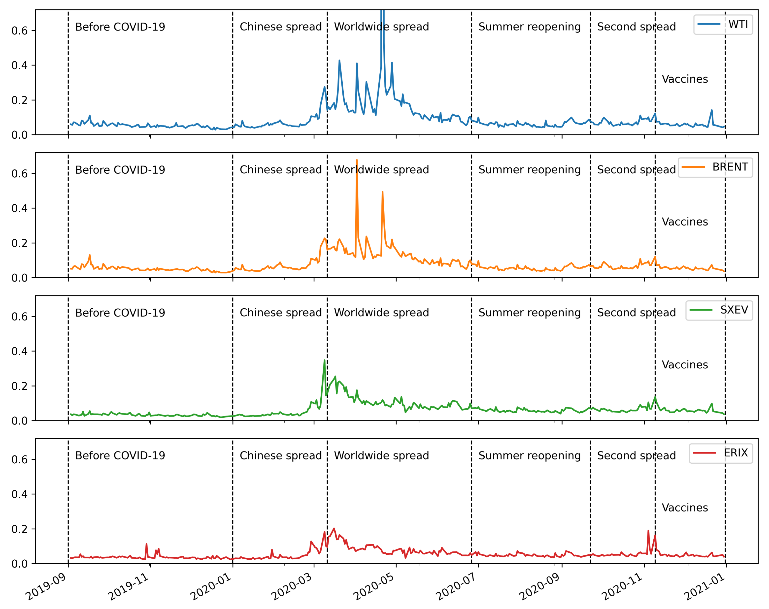
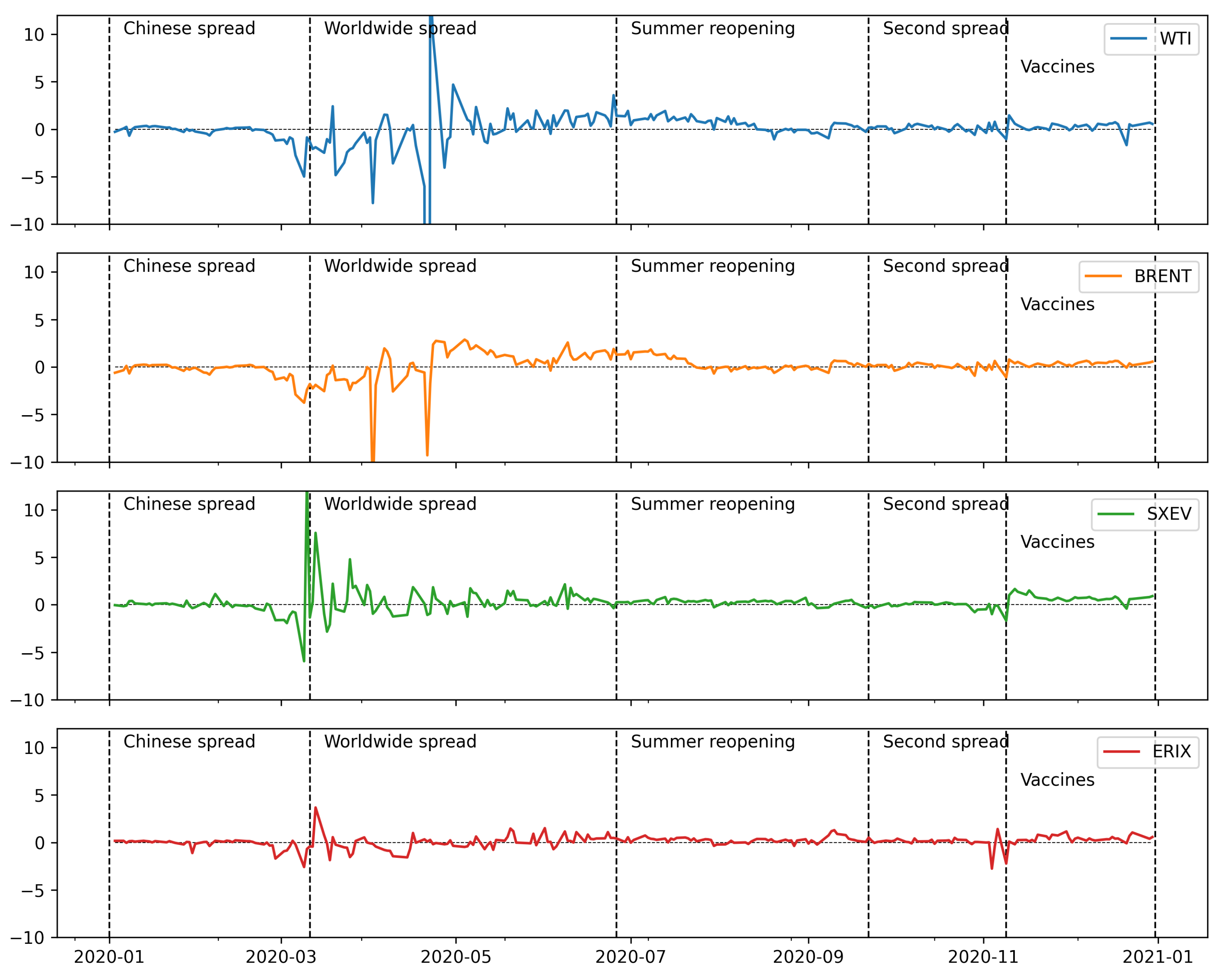
Table 1 shows also a high variability in the return series across the periods suggesting a possible volatility clustering. In fact, analyzing the daily volatility, computed as standard deviation of the 1-min returns, reported in Figure 2, and its average by period shown in

Table 2. Average daily volatility by period.

	WTI	BRENT	SXEV	ERIX
Before COVID-19	0.053	0.051	0.033	0.036
Chinese spread	0.072	0.069	0.051	0.047
Worldwide spread	0.286	0.140	0.110	0.081
Summer reopening	0.061	0.055	0.058	0.047
Second spread	0.071	0.066	0.063	0.056
Vaccines	0.060	0.055	0.060	0.051

, it is clear that between the Chinese and the worldwide spread the oil market faced a huge increase in volatility, that is less noticeable in the ERIX series. To enhance readability and comparability, the y-axis maximum values of the charts in Figure 2 have been limited to the same fixed value. Therefore, some outliers of the WTI series fall outside of the visible area. In this setting, we notice a smaller variability in the ERIX index which seems less affected by the COVID-19 events. On the contrary, the two oil contracts appear to be highly unstable around the pandemic spread.

Moreover,

Table 3. Correlation daily volatility computed as standard deviation of 1-min returns.

	WTI	BRENT	SXEV	ERIX
WTI	1.000000	0.495386	0.161341	0.089098
BRENT	0.495386	1.000000	0.665709	0.515934
SXEV	0.161341	0.665709	1.000000	0.876430
ERIX	0.089098	0.515934	0.876430	1.000000

reports a high volatility correlation between the Brent crude oil and the two indexes and between the SXEV and the ERIX index.

The evidence of volatility clustering, along with the high correlations, suggests that the application of the multivariate DCC-GARCH model from Engle [16] could be a good candidate to predict the oil market volatility.

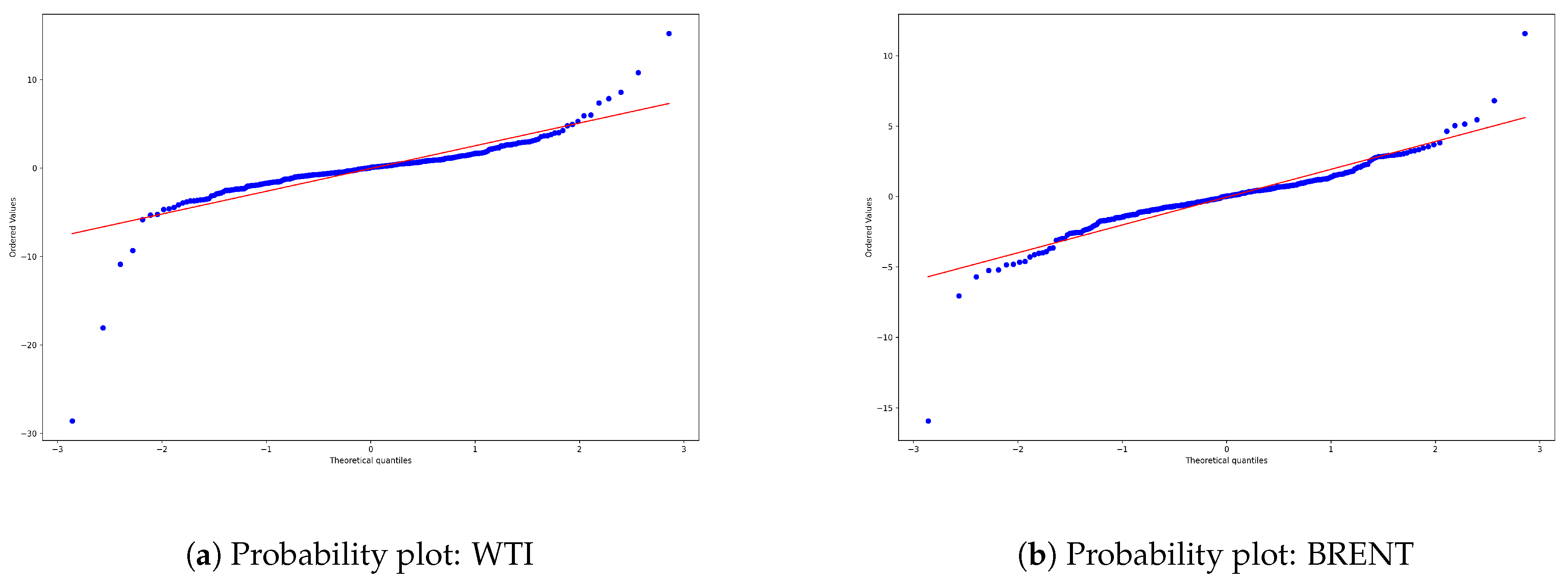
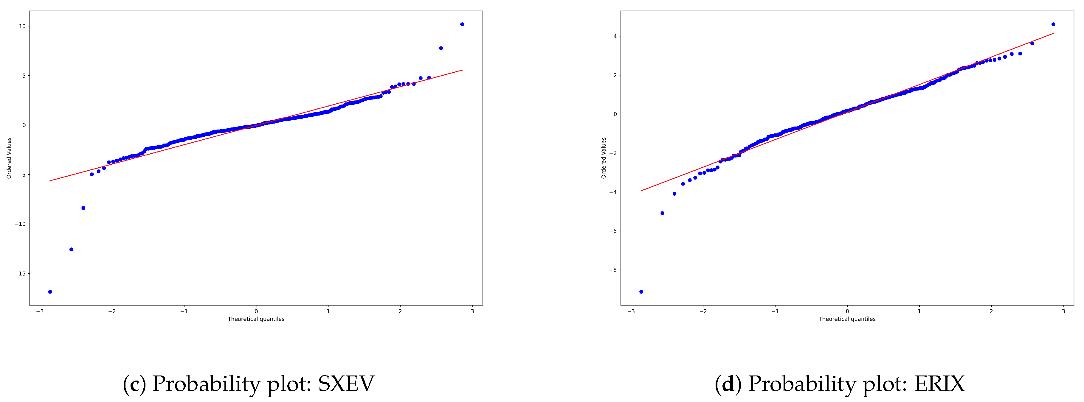
To this extent, we perform some summary statistics and diagnostic tests on the daily percentage log return of the four time series, as reported in

Table 4. Summary statistics and diagnostic tests of the daily percentage log returns. ADF: Augmented Dickey-Fuller unit root test; LM: Lagrange multiplier test statistic for ARCH effect; LB: Ljung-Box test of autocorrelation. The sample includes 325 daily observations.

	WTI	BRENT	SXEV	ERIX
Panel A: summary statistics (returns in %)
mean	−0.0532	−0.0480	−0.0539	0.1002
std	3.0212	2.1115	2.1455	1.4463
min	−28.5979	−15.9417	−16.8673	−9.1300
max	15.2176	11.5714	10.1787	4.6155
skew	−2.7681	−0.9060	−1.7426	−0.9769
kurt	30.3941	12.6321	16.5461	5.1810
Panel B: returns diagnostics
ADF	−8.561 ***	−18.506 ***	−6.859 ***	−6.953 ***
LM lag 1	100.513 ***	52.324 ***	2.532	26.523 ***
LM lag 2	104.585 ***	60.992 ***	4.530	26.527 ***
LM lag 3	104.263 ***	62.262 ***	46.043 ***	26.509 ***
Panel C: squared returns diagnostics
LB lag 1	101.744 ***	52.954 ***	2.563	26.829 ***
LB lag 2	116.732 ***	52.991 ***	5.018 *	28.240 ***
LB lag 3	117.808 ***	53.007 ***	50.329 ***	28.240 ***
Panel D: absolute returns diagnostics
LB lag 1	121.734 ***	51.150 ***	37.802 ***	27.021 ***
LB lag 2	171.196 ***	54.647 ***	63.006 ***	37.223 ***
LB lag 3	184.032 ***	55.471 ***	108.108 ***	37.992 ***

*** p < 0.01, ** p < 0.05, * p < 0.1.

. From Panel A of the table, the average return clearly appears close to zero for all series, and their distributions show fat tails, as denoted by the high levels of kurtosis. However, the probability plots in Figure 3 highlight that only a few extreme observations deviate from the normal distribution. Therefore, the use of the normal distribution in the model appears to be a good approximation. The Augmented Dickey-Fuller test confirms that all returns series are stationary.

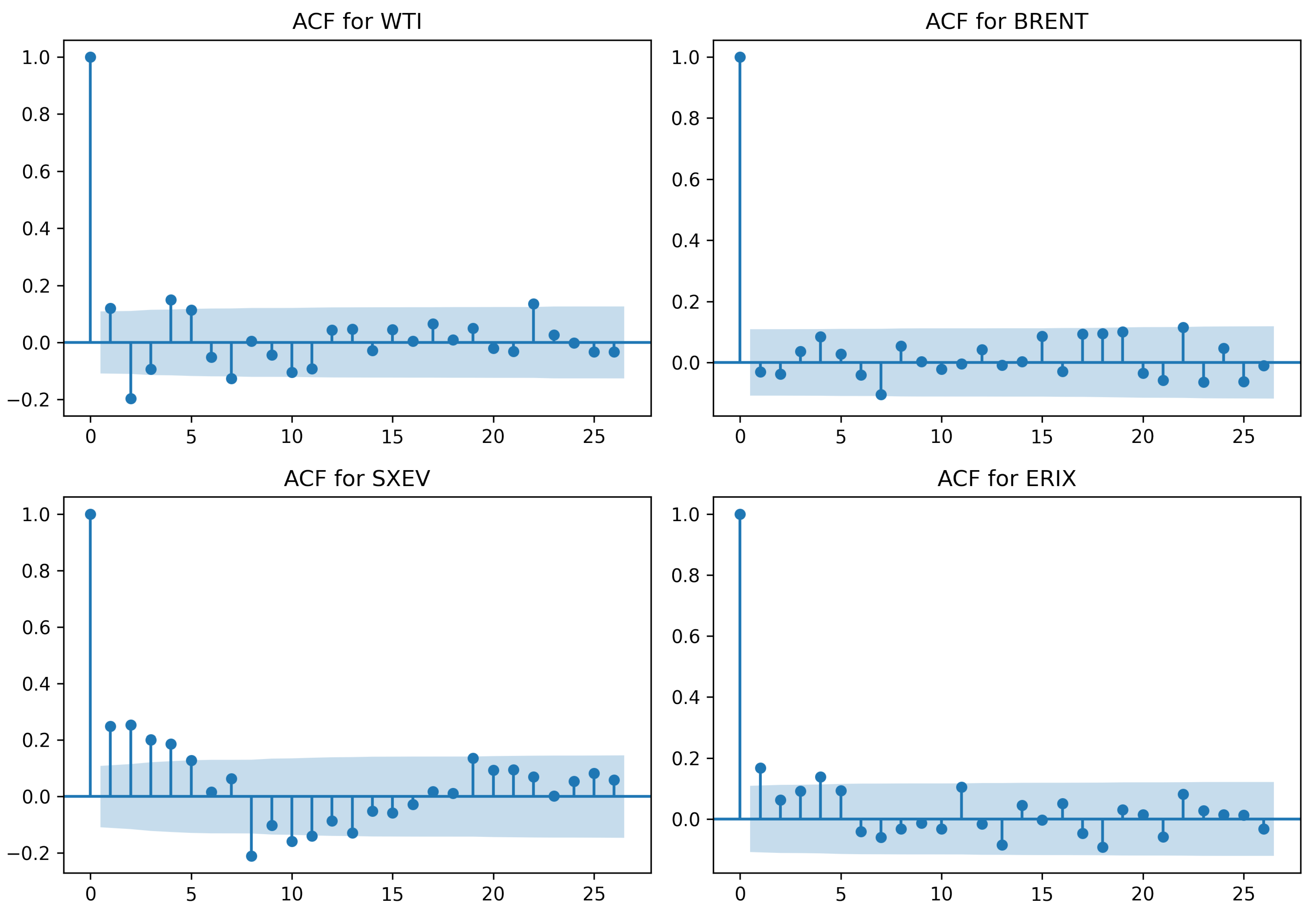
Modeling the return series requires the choice of a model for the mean. Analyzing the autocorrelation functions shown in Figure 4, there is evidence of the absence of serial correlation, with the only exception of the SXEV series. Therefore, considering that the multivariate model requires the same configuration for all series and that the average returns are almost zero, the use of a constant model for the mean of returns should suffice to reflect the characteristics of the selected series.

Moreover, the Lagrange Multiplier (LM) test from Engle [4] shows evidences of volatility clustering, as anticipated by the analysis of the daily standard deviation of intraday returns. The only exception is the SXEV series, for which we cannot reject the null hypothesis when analyzing the first two lags. However, the overall rejection of the null hypothesis of the absence of autocorrelation in the squared residuals permits us to model the volatility using the GARCH specification. In addition, we perform the Ljung-Box [29] test of autocorrelation on the squared and absolute returns (Panels C and D), which further confirms that the daily log return processes have a strong nonlinear dependence.

2.2. Methodology: DCC-GARCH

The price volatility analysis is performed using the DCC-GARCH, a class of multivariate GARCH estimator introduced by Engle [16] as a generalization of the constant conditional correlation estimator by Bollerslev [30].

Following the assumption of the constant mean as describe in the data section, we model the log returns of each series, i with the following equation:

$$r_{i,t}={\mu }_i+e_{i,t},$$

(1)

where ${\mu }_i$ is the constant mean, and $e_{i,t}$ is a zero mean white noise process.

The Dynamic Conditional Correlation model proposes a time-varying variance-covariance matrix with the following form:

$$H_t=D_t{R}_t{D}_t,$$

(2)

where $D_t$ is the diagonal matrix of the standard deviations of the demeaned returns, and $R_t$ is their conditional correlation matrix, such that the demeaned returns follow a multivariate normal distribution, $e_t\sim \mathcal{N}(0,H_t)$.

The full DCC model, in its scalar form, can be formulated as:

$$\begin{array}{cc}\hfill & D_t^2=diag\left\{{\omega }_i\right\}+diag\left\{{\kappa }_i\right\}\circ e_{t-1}{e}_{t-1}^{\prime }+diag\left\{{\lambda }_i\right\}\circ D_{t-1}^2,\hfill \\ \hfill & {ϵ}_t=D_t^{-1}{e}_t,\hfill \\ \hfill & R_t=Q_t^{\ast -1}{Q}_t{Q}_t^{\ast -1}\hfill \\ \hfill & Q_t=(1-\alpha -\beta )\overline{Q}+\alpha \left({ϵ}_{t-1}{ϵ}_{t-1}^{\prime }\right)+\beta Q_{t-1},\hfill \end{array}$$

(3)

where ∘ is the Hadamard product, ${ϵ}_t$ is the vector of the standardized errors, and $Q_t^{\ast }$ is the diagonal matrix with the square root of the diagonal elements of $Q_t$.

The first line in Equation (3) represents the variance equation of the univariate GARCH models, while, in the last line, there is the updating equation of the conditional correlation following a variance targeting approach with $\overline{Q}$ being the unconditional covariance matrix of the standardized errors estimated as $\overline{Q}=\frac{1}{T}{\sum }_{t=1}^T{ϵ}_t{ϵ}_t^T$.

To ensure stationarity with the variance targeting approach and that the matrices $Q_t$ are always positive definite, the following conditions apply:

$$\alpha ,\beta \ge 0,\alpha +\beta <1.$$

(4)

The estimation of the parameters, ${\omega }_i,{\kappa }_i,{\lambda }_i,\alpha$, and $\beta$, is performed with the 2-stage approach from Engle [16] maximizing the following log-likelihood function:

$$L=-\frac{1}{2}\sum _{t=1}^T\left(nlog\left(2\pi \right)+log|H_t|+e_t^{\prime }{H}_t^{-1}{e}_t\right).$$

(5)

2.3. Methodology: Price Leadership Share

The analysis of the correlation of the returns and their lagged values reported in

Table 5. Returns and lagged returns correlation.

	WTI	BRENT	SXEV	ERIX
WTI	1.000	0.495	0.161	0.089
BRENT	0.495	1.000	0.666	0.516
SXEV	0.161	0.666	1.000	0.876
ERIX	0.089	0.516	0.876	1.000
WTI L1	0.091	0.331	0.136	0.078
BRENT L1	0.141	0.635	0.589	0.499
SXEV L1	0.135	0.592	0.821	0.738
ERIX L1	0.117	0.481	0.749	0.732

shows a strong relation among the four series, as well as when we consider the lagged correlation in the second part of the table.

This high correlations suggest a potential dependence among the price series, which can be investigated following the approach proposed by De Blasis [25]. The author analyzes the price leadership in the gold market introducing a new measure beased on the Mixture Transition Distribution (MTD) model by Raftery [26] and extended to a multivariate setting by Ching et al. [23].

A sequence of $\mathrm{\Gamma }=\{1,2,\cdots ,\gamma \}$ random variables, ${\left\{S_t^{\alpha }\right\}}_{t\ge 0}$ with $\alpha \in \mathrm{\Gamma }$, taking values in the set $\mathcal{M}=\{1,\cdots ,m\}$, is called a multivariate Markov Chain when it satisfies the following multivariate Markov Property:

$$\begin{array}{c}\hfill \mathrm{Pr}[S_{t+1}^{\left(\alpha \right)}=j|(S_t^{\left(1\right)}=i_t^{\left(1\right)},S_{t-1}^{\left(1\right)}=i_{t-1}^{\left(1\right)},\cdots ,S_0^{\left(1\right)}=i_0^{\left(1\right)}),\cdots ,\\ \hfill (S_t^{\left(\gamma \right)}=i_t^{\left(\gamma \right)},S_{t-1}^{\left(\gamma \right)}=i_{t-1}^{\left(\gamma \right)},\cdots ,S_0^{\left(\gamma \right)}=i_0^{\left(\gamma \right)})]=\\ \hfill \mathrm{Pr}(S_{t+1}^{\left(\alpha \right)}=j|S_t^{\left(1\right)}=i_t^{\left(1\right)},\cdots ,S_t^{\left(\gamma \right)}=i_t^{\left(\gamma \right)}),\end{array}$$

(6)

which states that, for every series $\alpha \in \mathrm{\Gamma }$, the probability of being in state j depends on the state $i_1,\cdots ,i_{\gamma }$ occupied by all the available series one time step before.

To model the multivariate Markov chain without incurring in the problem of the high number of parameters to estimate, we can apply the MTD model, and the probability distribution of series $\alpha$ at time $t+1$ can be written as

$${\mathbf{A}}^{\left(\alpha \right)}(t+1)=\sum _{\beta =1}^{\gamma }{\mathbf{A}}^{\left(\beta \right)}\left(t\right)·{\lambda }_{\beta ,\alpha }·{\mathbf{P}}^{(\beta ,\alpha )},$$

(7)

where ${\mathbf{A}}^{\alpha }\left(t\right):=[A_1^{\left(\alpha \right)},\dots ,A_m^{\left(\alpha \right)}]$ and $A_i^{\left(\alpha \right)}\left(t\right):=Pr(S_t^{\left(\alpha \right)}=i)$ and ${\mathbf{P}}^{(\beta ,\alpha )}$ are the transition probability matrices containing the probabilities of moving from state i in series $\beta$ to state j in series $\alpha$. These transition probability matrices are subject to the following conditions:

$$0\le p_{i,j}\le 1,\sum _{j=1}^m{p}_{i,j}=1,$$

(8)

where $p_{i,j}$ is an element of ${\mathbf{P}}^{(\beta ,\alpha )}$.

This determination in (7) permits to estimate only ${\gamma }^2$ transition probability matrices ${\mathbf{P}}^{(\beta ,\alpha )}$ and one additional matrix containing ${\gamma }^2$ weights:

$$\begin{array}{cc}& Series\beta \\ Series\alpha & \begin{array}{cccc}1 & 2& \cdots & \gamma \end{array}\\ \begin{array}{c}1\\ 2\\ ⋮\\ \gamma \end{array}& \left[\begin{array}{cccc}{\lambda }_{1,1}& {\lambda }_{2,1}\hfill & \cdots & {\lambda }_{\gamma ,1}\\ {\lambda }_{1,2}& {\lambda }_{2,2}\hfill & \cdots & {\lambda }_{\gamma ,2}\\ ⋮& ⋮\hfill & \ddots & ⋮\\ {\lambda }_{1,\gamma }& {\lambda }_{2,\gamma }\hfill & \cdots & {\lambda }_{\gamma ,\gamma }\end{array}\right],\end{array}$$

(9)

which contains the portion of weights that each series $\beta$ has on the series $\alpha$ and that is subject to the following conditions

$$\sum _{\beta =1}^{\gamma }{\lambda }_{\beta ,\alpha }=1,{\lambda }_{\beta ,\alpha }\ge 0.$$

(10)

From the weight matrix, we can define a vector of price leadership share (PLS) as

$$PLS=\left[\frac{{\sum }_{\alpha =1}^{\gamma }{\lambda }_{1,\alpha }^{\ast }}{{\sum }_{\alpha =1}^{\gamma }{\sum }_{\beta =1}^{\gamma }{\lambda }_{\beta ,\alpha }^{\ast }},\cdots ,\frac{{\sum }_{\alpha =1}^{\gamma }{\lambda }_{\gamma ,\alpha }^{\ast }}{{\sum }_{\alpha =1}^{\gamma }{\sum }_{\beta =1}^{\gamma }{\lambda }_{\beta ,\alpha }^{\ast }}\right],$$

(11)

where

$${\lambda }_{\beta ,\alpha }^{\ast }=\left\{\begin{array}{cc}{\lambda }_{\beta ,\alpha }\hfill & \mathrm{if}\beta \ne \alpha \hfill \\ 0\hfill & \mathrm{if}\beta =\alpha \hfill \end{array}\right..$$

(12)

The PLS can help understanding which price series has the leadership over the full set of price series. The transition probabilities can be estimated through the standard Markov chain estimator and the weights can be estimated maximizing its log-likelihood function, as in De Blasis [25].

3. Empirical Results

3.1. DCC-GARCH Analysis

The DCC-GARCH analysis is performed on the daily returns computed as open to close returns. Results for the DCC-GARCH estimation are reported in

Table 6. DCC-GARCH(1,1) parameters. Panel A reports the univariate GARCH parameters for each series. Panel B reports the DCC-GARCH parameters for all four series. P-values in parentheses. LM: Lagrange multiplier test statistic for ARCH effect; LB: Ljung-Box test of autocorrelation.

Panel A: Univariate GARCH parameters
	WTI	BRENT	SXEV	ERIX
$\mu$	0.095	0.074	−0.032	0.177 ***
	(0.372)	(0.430)	(0.670)	(0.006)
$\omega$	1.161 ***	0.114	0.358	0.310
	(0.006)	(0.221)	(0.379)	(0.347)
$\kappa$	0.645 **	0.126 ***	0.483	0.252 **
	(0.036)	(0.005)	(0.100)	(0.033)
$\lambda$	0.283 **	0.851 ***	0.516 *	0.601 **
	(0.047)	(0.000)	(0.068)	(0.023)
Panel B: DCC-GARCH parameters
$\alpha$	0.050 ***
	(0.000)
$\beta$	0.887 ***
	(0.000)
Panel C: DCC-GARCH residuals diagnostic
	WTI	BRENT	SXEV	ERIX
LB	1.787	0.147	3.194 *	1.169
	(0.181)	(0.701)	(0.074)	(0.280)
LB ($resi{d}^2$)	0.996	0.698	0.038	0.917
	(0.318)	(0.404)	(0.846)	(0.338)

*** p < 0.01, ** p < 0.05, * p < 0.1.

. Panel A shows the univariate GARCH(1,1) analysis for each series. The $\kappa$ parameters, which measure the response of the volatility to external shocks, are above 0.10 for all series, implying that all contracts are responsive to market events. The WTI contract appears to be more sensitive, showing a higher coefficient of 0.645. These ARCH coefficients are significant for all series except for the SXEV index. This latter result was expected from the analysis performed in the data section where the time series showed a reduced significance in the ARCH tests, especially at the first two lags. On the contrary, the GARCH coefficients $\lambda$ are all significant, showing a high magnitude except for the WTI contract. This result suggests that large changes in the volatility of the WTI series take a shorter time to decay. Moreover, all series satisfy the mean-reverting condition, where $0<\kappa +\lambda <1$. Overall, there is evidence of the presence of conditional volatility in the daily data. Finally, Panel B reports the results of the multivariate DCC-GARCH(1,1) model, which are highly significant, thus showing the presence of the dynamic conditional correlation in the sample.

To assess the validity of the estimated parameters, we run a series of diagnostic tests on the standardized residuals of the DCC-GARCH model. Panel C of Table 6 reports the Ljung-Box statistics on the residuals and on the squared residuals. In all cases, we fail to reject the null hypothesis of no autocorrelation in the standardized residuals, indicating that the model is able to describe the conditional correlation of the four selected contracts.

To test wether the model is able to predict the volatility during the disrupting period of the COVID-19 pandemic, we perform the out-of-sample analysis on a rolling window basis. Specifically, the DCC-GARCH model is initially calibrated on the pre-COVID-19 period, i.e., 4-month period from 1 September to 31 December 2019. With the estimated parameters, we predict the variance covariance matrix for the following day. Then, we shift the 4-month window by one day and perform a new estimation of the DCC-GARCH model parameters along with a new prediction. Finally, we repeat the procedure up to 31 December 2020. The predicted volatilities for the full year are then compared with the computed daily volatilities based on the 1-min interval intraday returns. Figure 5 shows the prediction errors of the DCC-GARCH model for the five periods. As expected, the worldwide spread period reveals the highest variability of prediction errors, with the WTI series reaching a minimum value of −202.56 and a maximum value of 15.68. The effect of the information flow about the pandemic is reflected on the predictability power of the theoretical models. However, this effect is less evident on the renewable energy index, which was less affected by the COVID-19 pandemic, as shown in the data analysis section.

Moreover, a smaller effect is recalled between the second wave and the vaccine period, which both present a little instability in the overall market, as also reported in Figure 2 and in

Table 7. Prediction accuracy using RMSE by period.

	WTI	BRENT	SXEV	ERIX
Chinese spread	0.966618	0.914734	2.235645	0.552730
Worldwide spread	23.905959	2.445554	1.473740	0.804769
Summer reopening	0.868118	0.731535	0.354176	0.406645
Second spread	0.353359	0.322304	0.306062	0.582914
Vaccines	0.579485	0.447151	0.859321	0.622851

, which shows the root mean square error (RMSE) by period for the four series. Again, the WTI predictability during the worldwide spread is the most affected, followed by the BRENT one. It is also important to notice that the summer reopening depicts a lower predictability (higher RMSE) than the second spread, but this is due to the calibration window that overlaps the worldwide spread period. In addition, the SXEV index shows a lower predictability during the Chinese spread.

3.2. Price Leadership Analysis

To analyze the linkages between the series in terms of prices, we apply the price leadership share model by De Blasis [25]. The model is computed at 1-min interval for the six subperiods. To estimate the transition probability matrices and the ${\lambda }_{\beta ,\alpha }$ weights in (7), we have to categorize the price returns into discrete states of the Markov chain. In general, building a Markov chain with many states means having a model that better captures the full dynamic of the system. However, the more states we include, the more parameters we need to estimate. This means that the application would need a greater availability of observations. To obtain a trade-off between a good representation of the system’s dynamics and a sound estimation of the parameters, we model our multivariate Markov chain with a three-state chain. The central state coincides with the zero return and the other states include the positive and negative returns, respectively. To avoid transitions from one state to another due to the small market microstructure noise, the central state includes all returns within one standard deviation around the zero return. Moreover, it is worth to mention that adding more states to the chain will only slightly affect the precision of the estimation of the weights, and consequently, of the price leadership shares, as highlighted in Reference [25].

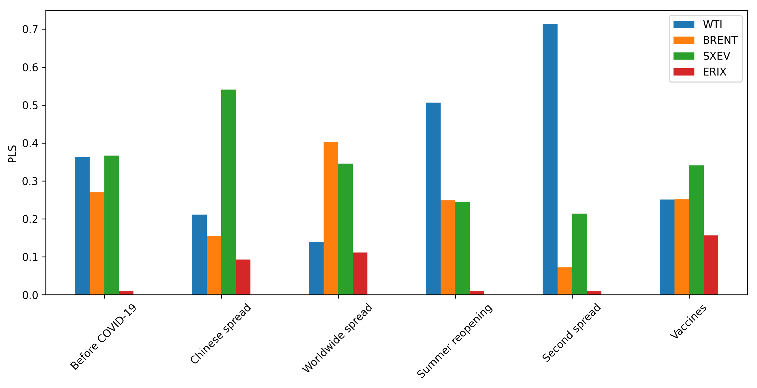
Figure 6 reports the PLS values for the six periods. The first clear evidence is that the ERIX index appears to be not so relevant in the price leadership, especially before the pandemic spread, during the summer reopening, and the second spread. Nonetheless, this result was expected if we consider the initial analysis in the data section. In fact, the ERIX index price series in Figure 1 follows a completely different trend compared to the other series, and the volatility of the ERIX in Figure 2 is much lower than the other series. In addition, the two oil contracts and the SXEV index are more related with each other, thus allowing for more spillover of price influence. However, it is worth to notice a few increases of the price leadership share of the ERIX index during the toughest periods of the pandemic, demonstrating a lower capacity of the other series to maintain a strong leadership in prices.

Overall, the COVID-19 pandemic disrupted the price leadership relations. In fact, before the pandemic, the price leadership share of the three oil related series appeared to be leveled. An equilibrium in the PLS shows a reduced concentration of information, therefore it is not possible to identify a clear leader. However, this situation flips during the Chinese spread, with the SXEV index taking the leadership over the other contracts. This reflects the huge drop that the two oil contracts faced during the pandemic spread, especially for the WTI. A slight change is noticeable during the worldwide spread when the BRENT contract shares the leadership with the SXEV index. Then, the WTI takes the leading position position during the summer reopening and the second spread, to finally come back to an almost normal situation during the vaccine period, but with the inclusion of the ERIX index in the share. The PLS values for the vaccine period are almost the same, showing a lack of concentration of the price leadership.

4. Discussion

In this paper, we analyzed the effect of COVID-19 on the volatility spillover between the oil market and two European indexes, an oil-related index and a renewable energies index. We modeled the volatility interactions using the DCC-GARCH model, which has been extensively used in the study of financial markets. In general, this multivariate GARCH model has proven to help model the volatility in periods of financial stability, but also during financial crises [21]. Indeed, there are many extensions and variations of the DCC-GARCH model proposed in the current literature. All these models have proven to be superior in modeling various aspects of the financial time series. However, the availability of programming tools for such models is limited. Therefore, the DCC-GARCH remains a preferred choice, especially for its simple two-stage estimation process.

Nonetheless, the COVID-19 presented a considerable disruption in financial markets with the WTI crude oil showing negative prices for the first time. The current literature reports a positive ability of DCC-GARCH to model the volatility linkages during the financial crisis. However, it fails to test the predictability of the model. Ding and Vo [17] found volatility interactions between the oil and foreign exchange markets only during the 2008 financial crisis. On the contrary, they reported that both markets respond to shocks simultaneously when the markets are relatively calm. Similarly, Brayek et al. [18] found the existence of an impact between oil prices and exchange rates during the crisis, as well as Celik [21], who reported the financial contagion during the subprime crisis. Moreover, Singhal and Ghosh [19] found evidence of co-movements between crude oil and the Indian stock market.

Our results from the application of the DCC-GARCH model to two crude oil contracts and two oil-related and renewable indexes during the extreme conditions of the COVID-19 pandemic confirm the evidence of volatility spillover between the time series. The parameters estimation of the model and the residual diagnostics clearly show the presence of co-movements in these markets. Moreover, the price leadership share analysis reveals that the disruption of the COVID-19 pandemic introduced a leadership identification crisis among the series. It is evident from Figure 6 that the ERIX index, which was less affected by the pandemic, was leading the price movements during the worldwide spread and that these results were flipped going back to a calmer and normal period after the markets absorbed the news of the virus. These findings from this innovative model are aligned with and support the presence of the volatility spillover between the series.

However, when assessing the accuracy of the predictability of the DCC-GARCH model, the results show that the model fails its prediction in the period of higher instability, i.e., the worldwide spread of the disease. On the contrary, the model appears to be quite good during calmer periods, with some smaller instabilities over other periods with the presence of COVID-19 related events.

These last findings highlight the necessity to carefully consider the model when applying it to periods of great instability. Besides, it is important to elaborate on the causes of this discrepancy in the results. Further studies might analyze whether the observation of co-movements during unstable periods is due to real causes or it is due to a model design.

5. Conclusions

The COVID-19 pandemic has changed societies worldwide in many aspects. In this work, we tried to understand the influences of virus spreading on oil and energy markets. More precisely, we investigated the behavior of volatility linkages between oil and renewable energy firms by analyzing two crude oil futures prices, namely the West Texas Intermediate crude oil futures contract (WTI) and the Brent crude oil futures contract (BRENT), and two indices, namely the STOXX Europe 600 oil & gas index (SXEV) and the European renewable energy index (ERIX). The period between September 2019 and January 2021 was divided into 6 subgroups according to the pandemic stages. We found that, during the worldwide spread (between March and July 2020), there has been a fast growing in volatility for all energy firms. This phenomenon has been much stronger for oil firms with respect to renewable energy firms. Furthermore, during the worldwide spread, the ability to forecast volatility has decreased. Besides, we investigated the price leadership share, showing that the COVID-19 pandemic disrupted the price leadership relation amongst the four analyzed time series.

References

1. Goodell, J.W. COVID-19 and Finance: Agendas for Future Research. Financ. Res. Lett. 2020, 35, 101512. [Google Scholar] [CrossRef]
2. Bouri, E.; Demirer, R.; Gupta, R.; Pierdzioch, C. Infectious Diseases, Market Uncertainty and Oil Market Volatility. Energies 2020, 13, 4090. [Google Scholar] [CrossRef]
3. Corbet, S.; Goodell, J.W.; Günay, S. Co-Movements and Spillovers of Oil and Renewable Firms under Extreme Conditions: New Evidence from Negative WTI Prices during COVID-19. Energy Econ. 2020, 92, 104978. [Google Scholar] [CrossRef] [PubMed]
4. Engle, R.F. Autoregressive Conditional Heteroscedasticity with Estimates of the Variance of United Kingdom Inflation. Econometrica 1982, 50, 987–1007. [Google Scholar] [CrossRef]
5. Bekaert, G.; Harvey, C.R. Emerging Equity Market Volatility. J. Financ. Eco. 1997, 43, 29–77. [Google Scholar] [CrossRef] [Green Version]
6. Bollerslev, T.; Ole Mikkelsen, H. Modeling and Pricing Long Memory in Stock Market Volatility. J. Econom. 1996, 73, 151–184. [Google Scholar] [CrossRef]
7. Engle, R.F. ARCH: Selected Readings; Oxford University Press: Oxford, UK, 1995. [Google Scholar]
8. Brailsford, T.J.; Faff, R.W. An Evaluation of Volatility Forecasting Techniques. J. Bank. Financ. 1996, 20, 419–438. [Google Scholar] [CrossRef]
9. Choudhry, T. Stock Market Volatility and the Crash of 1987: Evidence from Six Emerging Markets. J. Int. Money Financ. 1996, 15, 969–981. [Google Scholar] [CrossRef]
10. Bollerslev, T. Generalized Autoregressive Conditional Heteroskedasticity. J. Econom. 1986, 31, 307–327. [Google Scholar] [CrossRef] [Green Version]
11. Antoniou, A.; Holmes, P. Futures Trading, Information and Spot Price Volatility: Evidence for the FTSE-100 Stock Index Futures Contract Using GARCH. J. Bank. Financ. 1995, 19, 117–129. [Google Scholar] [CrossRef]
12. Franses, P.H.; Dijk, D.V. Forecasting Stock Market Volatility Using (Non-Linear) Garch Models. J. Forecast. 1996, 15, 229–235. [Google Scholar] [CrossRef]
13. Dueker, M.J. Markov Switching in GARCH Processes and Mean-Reverting Stock-Market Volatility. J. Bus. Econ. Stat. 1997, 15, 26–34. [Google Scholar] [CrossRef] [Green Version]
14. Marcucci, J. Forecasting Stock Market Volatility with Regime-Switching GARCH Models. Stud. Nonlinear Dyn. Econ. 2005, 9, 1–55. [Google Scholar] [CrossRef]
15. D’Amico, G.; Gismondi, F.; Petroni, F.; Prattico, F. Stock Market Daily Volatility and Information Measures of Predictability. Phys. A Stat. Mech. Appl. 2019, 518, 22–29. [Google Scholar] [CrossRef]
16. Engle, R. Dynamic Conditional Correlation. J. Bus. Econ. Stat. 2002, 20, 339–350. [Google Scholar] [CrossRef]
17. Ding, L.; Vo, M. Exchange Rates and Oil Prices: A Multivariate Stochastic Volatility Analysis. Q. Rev. Econ. Financ. 2012, 52, 15–37. [Google Scholar] [CrossRef]
18. ben Brayek, A.; Sebai, S.; Naoui, K. A Study of the Interactive Relationship between Oil Price and Exchange Rate: A Copula Approach and a DCC-MGARCH Model. J. Econ. Asymmetries 2015, 12, 173–189. [Google Scholar] [CrossRef]
19. Singhal, S.; Ghosh, S. Returns and Volatility Linkages between International Crude Oil Price, Metal and Other Stock Indices in India: Evidence from VAR-DCC-GARCH Models. Resour. Policy 2016, 50, 276–288. [Google Scholar] [CrossRef]
20. Hou, K.; Moskowitz, T.J. Market Frictions, Price Delay, and the Cross-Section of Expected Returns. Rev. Financ. Stud. 2005, 18, 981–1020. [Google Scholar] [CrossRef]
21. Celık, S. The More Contagion Effect on Emerging Markets: The Evidence of DCC-GARCH Model. Econ. Model. 2012, 29, 1946–1959. [Google Scholar] [CrossRef]
22. Bauwens, L.; Laurent, S.; Rombouts, J.V.K. Multivariate GARCH Models: A Survey. J. Appl. Econom. 2006, 21, 79–109. [Google Scholar] [CrossRef] [Green Version]
23. Ching, W.K.; Fung, E.S.; Ng, M.K. A Multivariate Markov Chain Model for Categorical Data Sequences and Its Applications in Demand Predictions. IMA J. Manag. Math. 2002, 13, 187–199. [Google Scholar] [CrossRef]
24. D’Amico, G.; De Blasis, R. A Multivariate Markov Chain Stock Model. Scand. Actuar. J. 2020, 2020, 272–291. [Google Scholar] [CrossRef]
25. De Blasis, R. The Price Leadership Share: A New Measure of Price Discovery in Financial Markets. Ann. Financ. 2020, 16, 381–405. [Google Scholar] [CrossRef]
26. Raftery, A.E. A Model for High-Order Markov Chains. J. R. Stat. Soc. Ser. B 1985, 47, 528–539. [Google Scholar] [CrossRef]
27. Safi, M. Coronavirus: Key Moments–Timeline. The Guardian. 2020. Available online: https://www.theguardian.com/world/ng-interactive/2020/dec/14/coronavirus-2020-timeline-covid-19 (accessed on 6 January 2021).
28. A Timeline of COVID-19 Developments in 2020. Available online: https://www.ajmc.com/view/a-timeline-of-covid19-developments-in-2020 (accessed on 6 January 2021).
29. Ljung, G.M.; Box, G.E.P. On a Measure of Lack of Fit in Time Series Models. Biometrika 1978, 65, 297–303. [Google Scholar] [CrossRef]
30. Bollerslev, T. Modelling the Coherence in Short-Run Nominal Exchange Rates: A Multivariate Generalized Arch Model. Rev. Econ. Stat. 1990, 72, 498–505. [Google Scholar] [CrossRef]
Figure 1. Price series in U.S. dollars of the four contracts from 1 September 2019 to 31 December 2020. Transactions are sampled at 1-min frequency from 8:00 a.m. to 4:50 p.m. London time.
Energies 14 02608 g001
Figure 2. Daily volatility series of the four contracts from 1 September 2019 to 31 December 2020, computed as standard deviation of 1-min returns from 8:00 a.m. to 4:50 p.m. London time.
Energies 14 02608 g002
Figure 3. Probability plots of the daily percentage log returns of the four indexes.
Energies 14 02608 g003aEnergies 14 02608 g003b
Figure 4. Autocorrelation function for the daily percentage log returns.
Energies 14 02608 g004
Figure 5. Time series of deviations between predicted volatilities through DCC-GARCH(1,1) model and daily volatilities estimated as standard deviations of 1-min returns.
Energies 14 02608 g005
Figure 6. Price Leadership Share by period.
Energies 14 02608 g006