
Optimization of Design Variables of a Phase Change Material Storage Tank and Comparison of a 2D Implicit vs. 2D Explicit Model


 , ,
, ,  ,
,  and
and 
Abstract
1. Introduction
2. Materials and Methods
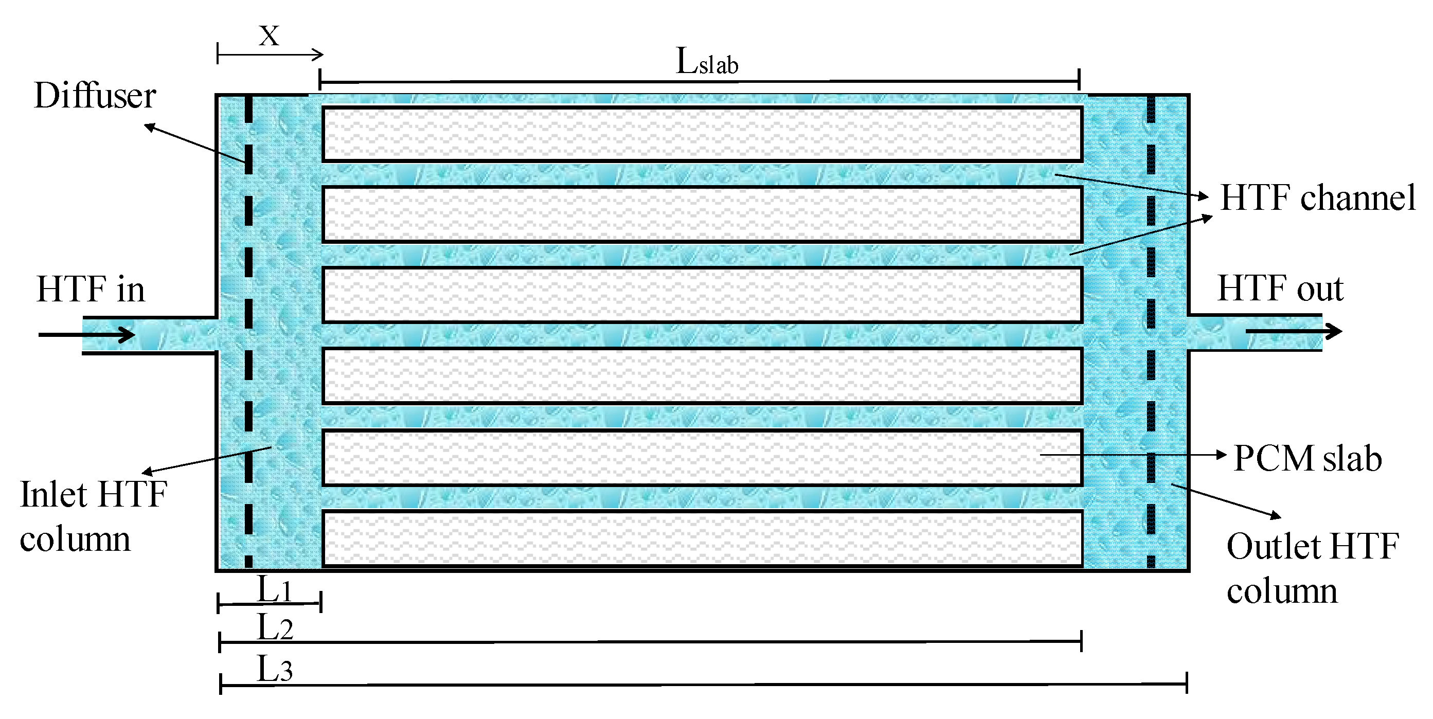
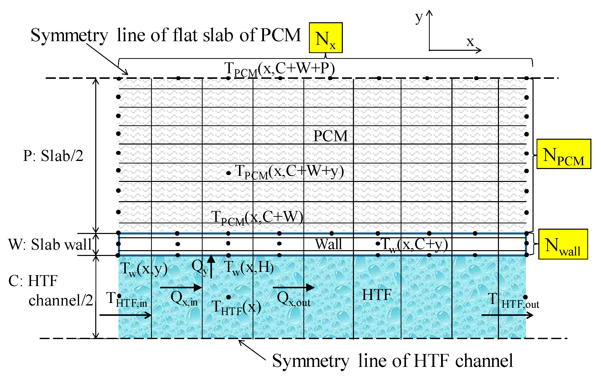
2.1. Numerical Model (2D)
- The density and thermal conductivity of the PCM were considered constant in each of the phases and also during the phase change.
- The phase change was taken into account through an equivalent specific heat capacity [19]. During the phase change, the temperature dependence on the PCM specific heat capacity had a trapezium shape centred on the melting temperature of the PCM with an upper base of the trapezium of 1 °C. It was an analogous methodology to the one presented by Farid [20], who used a triangle shape distribution, which was found to be successful for modelling heat transfer in PCM.
- The PCM was considered homogeneous and isotropic.
- All the PCM was initially at the same temperature. The initial temperature of the HTF inside the tank and of the plastic container has been also set to the same temperature.
- Thermal losses to the environment were not considered.
- All the slabs had symmetrical thermal behaviour with respect to the horizontal plane that crosses their centre.
- The mass flow was divided evenly between each HTF channel.
- Natural convection was neglected inside the liquid phase of the PCM due to the thin, flat nature of the slabs and their horizontal layout [21].
- Constant Cp of the HTF was considered since according to Zsembinszki et al. [6] the density and specific heat of the HTF could be considered constant to reduce the computational time as they have less importance in the mean absolute percentage error (MAPE).
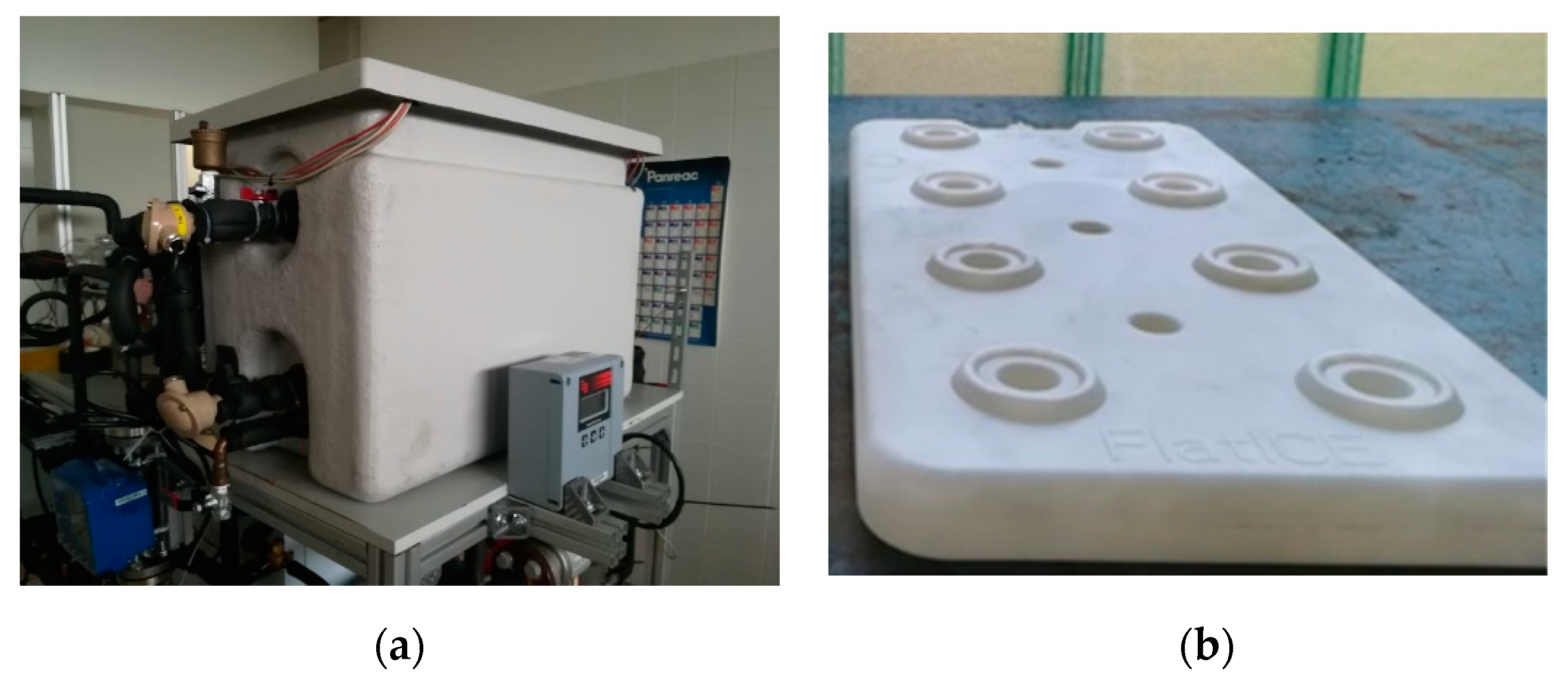
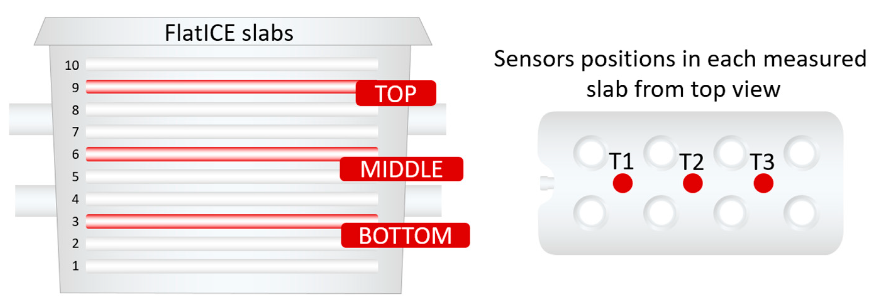
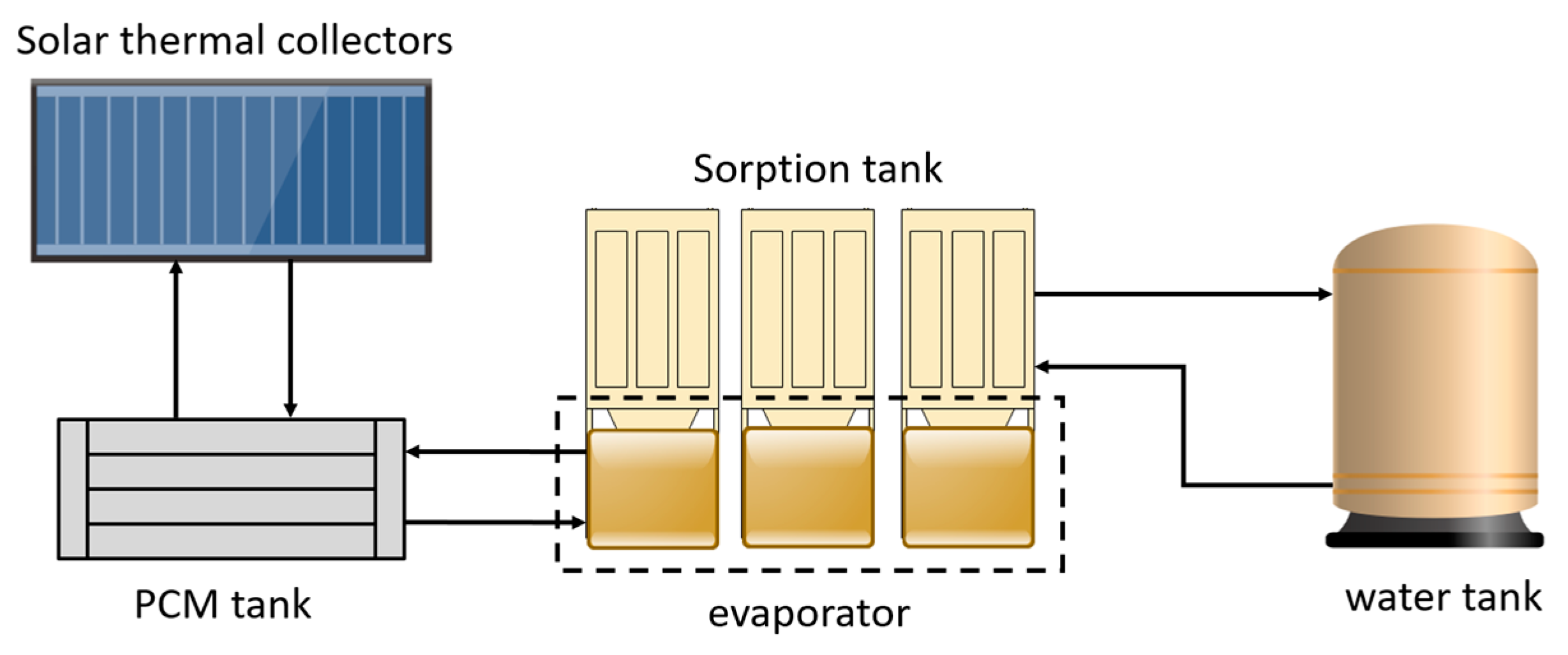
2.2. Experimental Set-Up
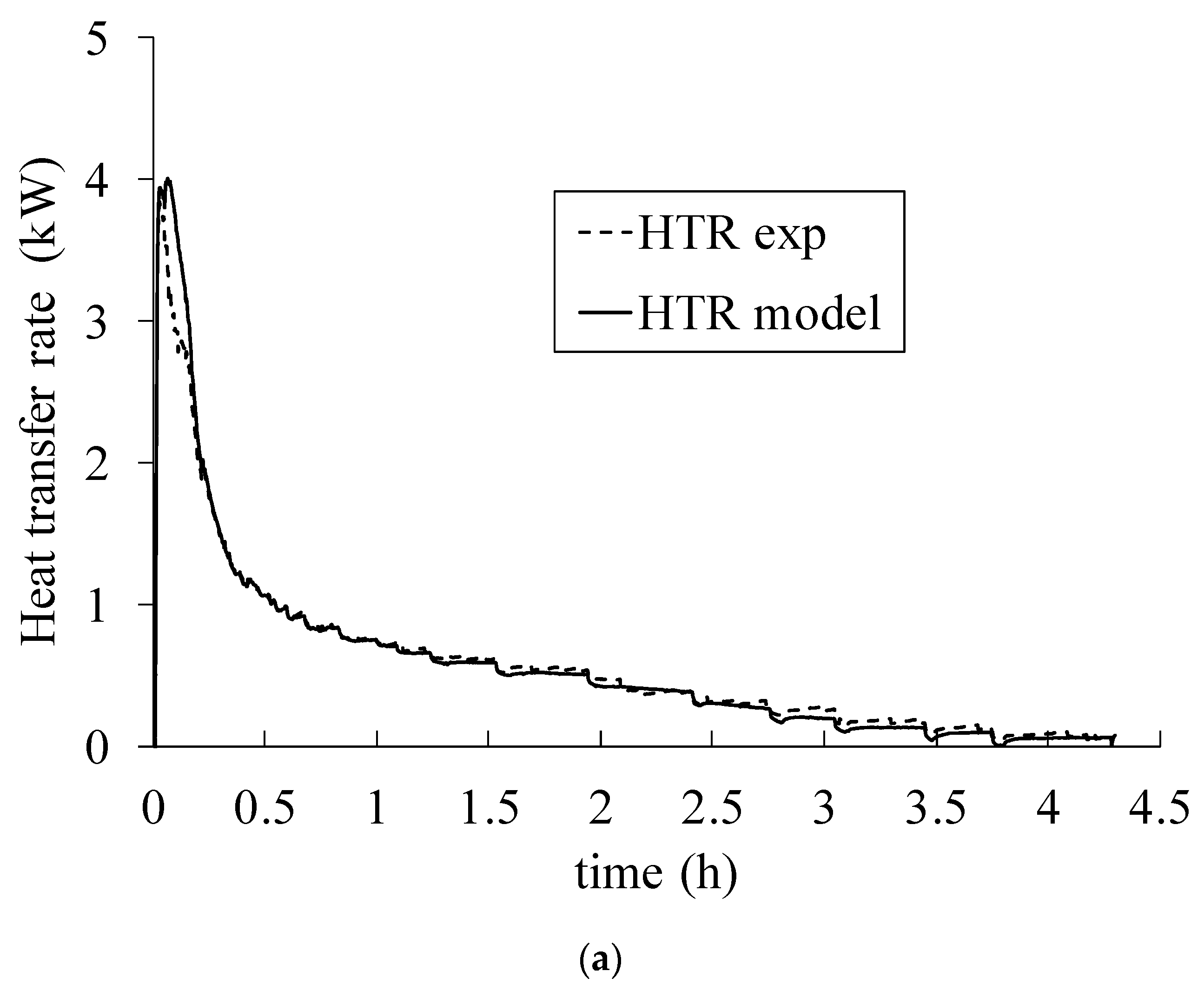
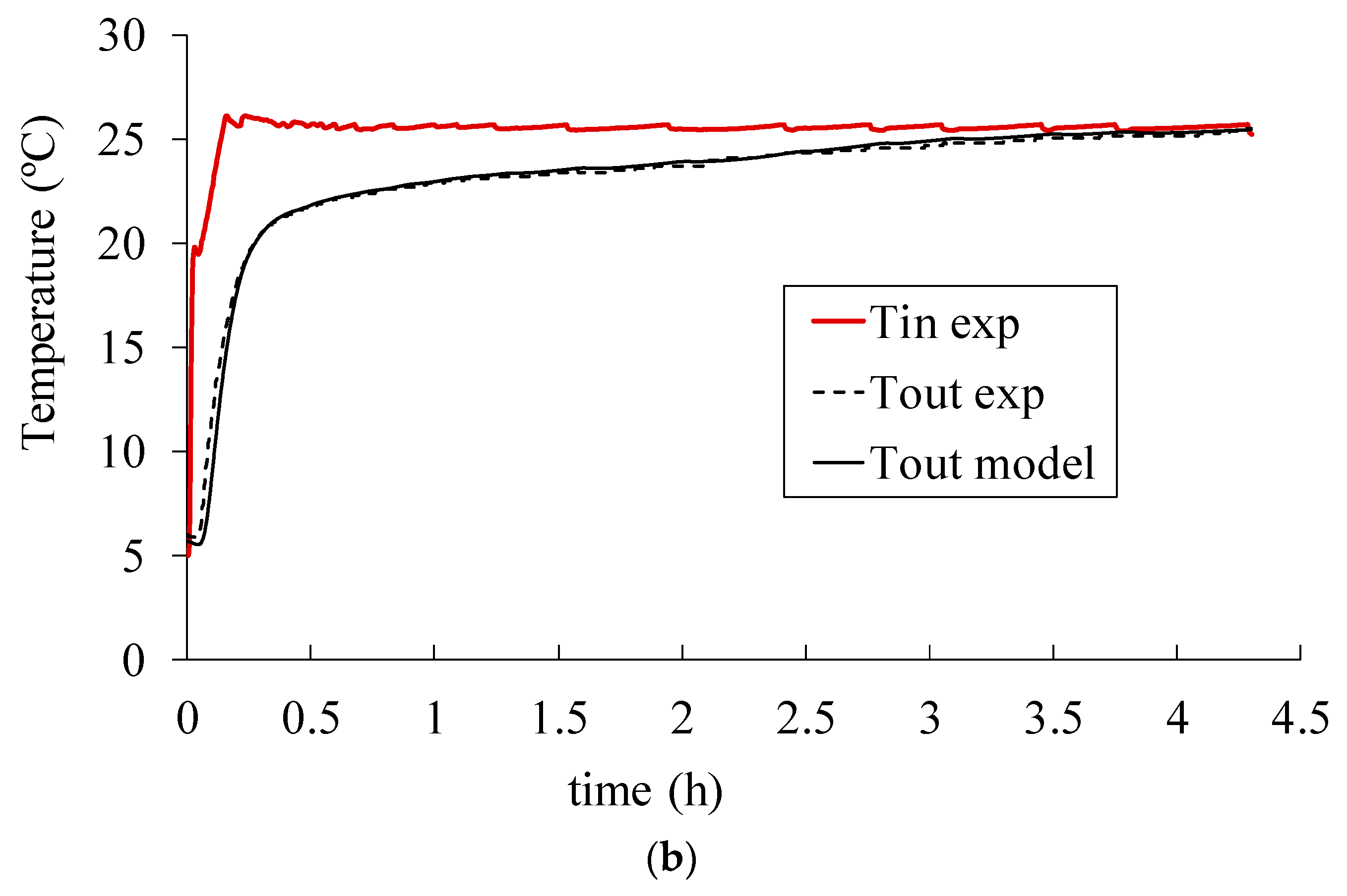
2.3. Model Validation
2.4. Design Optimization of the System for Real-Scale Application
2.5. Comparison between 2D Implicit and 2D Explicit Model
3. Results and Discussion
3.1. Optimization of Design Variables of the PCM Tank
3.2. Comparison of Implicit and Explicit 2D Schemes during Discharge
4. Conclusions
Author Contributions
Funding
Institutional Review Board Statement
Informed Consent Statement
Data Availability Statement
Acknowledgments
Conflicts of Interest
Nomenclature
| Symbols | |
| h | heat transfer coefficient, W/m2K |
| Cp | specific heat, kJ/kgK |
| mass flow rate, kg/h | |
| H | total volumetric enthalpy, W/m2K |
| k | thermal conductivity, W/mK |
| L | distance, m |
| T | temperature, K |
| Q | heat transfer rate, kW |
| N | number of nodes |
| n | number of time-steps of simulation |
| t | time |
| R | function which depend on measured parameters |
| w | uncertainties associated to independent parameters |
| W | estimated uncertainty in final result, value-dependent |
| a | independent measured parameters |
| Subscript | |
| HTF | heat transfer fluid |
| X | x-axis |
| Y | y-axis |
| in | inlet |
| out | outlet |
| wall | container wall |
| 0 | initial |
| tank | storage unit |
| sim | simulated |
| ref | reference |
| t | time-step under study |
References
- Pirasaci, T. Investigation of phase state and heat storage form of the phase change material (PCM) layer integrated into the exterior walls of the residential-apartment during heating season. Energy 2020, 207, 118176. [Google Scholar] [CrossRef]
- De Gracia, A.; Navarro, L.; Castell, A.; Cabeza, L.F. Numerical study on the thermal performance of a ventilated facade with PCM. Appl. Therm. Eng. 2013, 61, 371–380. [Google Scholar] [CrossRef]
- Royo, P.; Acevedo, L.; Ferreira, V.J.; García-armingol, T.; Ana, M.L. High-temperature PCM-based thermal energy storage for industrial furnaces installed in energy-intensive industries. Energy 2019, 173, 1030–1040. [Google Scholar] [CrossRef]
- Prieto, C.; Cabeza, L.F. Thermal energy storage (TES) with phase change materials (PCM) in solar power plants (CSP). Concept and plant performance. Appl. Energy 2019, 254, 113646. [Google Scholar] [CrossRef]
- Gil, A.; Oro, E.; Miró, L.; Peiro, G.; Ruiz, Á.; Salmeron, J.M.; Cabeza, L.F. Experimental analysis of hydroquinone used as phase change material (PCM) to be applied in solar cooling refrigeration. Int. J. Refrig. 2014, 39, 95–103. [Google Scholar] [CrossRef]
- Zsembinszki, G.; Moreno, P.; Solé, C.; Castell, A.; Cabeza, L.F. Numerical model evaluation of a PCM cold storage tank and uncertainty analysis of the parameters. Appl. Therm. Eng. 2014, 67, 16–23. [Google Scholar] [CrossRef]
- D’Avignon, K.; Kummert, M. Modeling horizontal storage tanks with encapsulated phase change materials for building performance simulation. Sci. Technol. Built Environ. 2018, 24, 327–342. [Google Scholar] [CrossRef]
- Halawa, E.; Bruno, F.; Saman, W. Numerical analysis of a PCM thermal storage system with varying wall temperature. Energy Convers. Manag. 2005, 46, 2592–2604. [Google Scholar] [CrossRef]
- Voller, V. Fast implicit finite difference method for the analysis of phase change problems. Numer. Heat Transf. Part B Fundam. 1990, 155–169. [Google Scholar] [CrossRef]
- De Gracia, A.; David, D.; Castell, A.; Cabeza, L.F.; Virgone, J. A correlation of the convective heat transfer coef fi cient between an air fl ow and a phase change material plate. Appl. Therm. Eng. 2013, 51, 1245–1254. [Google Scholar] [CrossRef]
- Simard, A.P.; Lacroix, M. Study of the thermal behavior of a latent heat cold storage unit operating under frosting conditions. Energy Convers. Manag. 2003, 44, 1605–1624. [Google Scholar] [CrossRef]
- Halawa, E.; Saman, W.; Bruno, F. A phase change processor method for solving a one-dimensional phase change problem with convection boundary. Renew. Energy 2010, 35, 1688–1695. [Google Scholar] [CrossRef]
- Liu, M.; Saman, W.; Bruno, F. Validation of a mathematical model for encapsulated phase change material flat slabs for cooling applications. Appl. Therm. Eng. 2011, 31, 2340–2347. [Google Scholar] [CrossRef]
- Bony, J.; Citherlet, S. Numerical model and experimental validation of heat storage with phase change materials. Energy Build. 2007, 39, 1065–1072. [Google Scholar] [CrossRef]
- Newton, B.J. Modelling of Solar Storage Tanks; University of Wisconsin-Madison: Madison, WI, USA, 1995. [Google Scholar]
- Serawa, A.; Jutang, A.; Razali, N.; Othman, H.; Hishamuddin, H. Draining of Water Tank using Runge-Kutta Methods. Int. J. Recent Technol. Eng. 2020, 8, 2277–3878. [Google Scholar] [CrossRef]
- Lei, Z.; Hongzhou, J. Variable step euler method for real-time simulation. In Proceedings of the 2nd International Conference on Computer Science and Network Technology, Changchun, China, 29–31 December 2012; pp. 2006–2010. [Google Scholar]
- Van Rossum, G.; Drake, F.L., Jr. Python Tutorial; Centrum voor Wiskunde en Informatica: Amsterdam, The Netherlands, 1995. [Google Scholar]
- Lamberg, P.; Lehtiniemi, R.; Henell, A.M. Numerical and experimental investigation of melting and freeizing processes in phase change material storage. Int. J. Therm. Sci. 2004, 43, 277–287. [Google Scholar] [CrossRef]
- Farid, M.M. A new approach in the calculation of heat transfer with phase change. In Proceedings of the 9th International Congress on Energy and Environment, Miami Beach, FL, USA, 11–13 December 1989; pp. 1–19. [Google Scholar]
- Zivkovic, B.; Fujii, I. An analysis of isothermal phase change of phase change material within rectangular and cylindrical containers. Sol. Energy 2001, 70, 51–61. [Google Scholar] [CrossRef]
- Kakaç, S.; Shah, R.K.; Aung, W. Handbook of Single-Phase Convective Heat Transfer; Wiley: Hoboken, NJ, USA, 1987; ISBN 0471817023/9780471817024. [Google Scholar]
- Patankar, S. Numerical Heat Transfer; Hemisphere Publications: London, UK, 1980. [Google Scholar]
- PCM Products. Available online: http://www.pcmproducts.net/ (accessed on 15 January 2019).
- Holman, J. Experimental Methods for Engineers, 8th ed.; McGraw-Hill: New York, NY, USA, 2012; ISBN 0073529303. [Google Scholar]
- Bergstra, J.; Yamins, D.; Cox, D.D. Making a science of model search: Hyperparameter optimization in hundreds of dimensions for vision architectures. In Proceedings of the 30th International Conference on Machine Learning, ICML 2013, (PART 1), Atlanta, GA, USA, 16–21 June 2013; pp. 115–123. [Google Scholar]
- Shevchuk, Y. NeuPy—Neural Networks in Python. Available online: http://neupy.com/2016/12/17/hyperparameter_optimization_for_neural_networks.html#tree-structured-parzen-estimators-tpe (accessed on 2 February 2021).
- Bergstra, J.; Bardenet, R.; Bengio, Y.; Kégl, B. Algorithms for Hyper-Parameter Optimization. Adv. Neural Inf. Process. Syst. 24 2011. [Google Scholar]
- Çengel, Y.A. Heat Transfer. A practical approach 2nd Edition—Annex—Table 8-1; McGrawHill: New York, NY, USA, 2002; ISBN 978-0072458930. [Google Scholar]
- Romaní, J.; Belusko, M.; Alemu, A.; Cabeza, L.F.; de Gracia, A.; Bruno, F. Control concepts of a radiant wall working as thermal energy storage for peak load shifting of a heat pump coupled to a PV array. Renew. Energy 2018, 118, 489–501. [Google Scholar] [CrossRef]
- de Gracia, A.; Barzin, R.; Fernández, C.; Farid, M.M.; Cabeza, L.F. Control strategies comparison of a ventilated facade with PCM—energy savings, cost reduction and CO2 mitigation. Energy Build. 2016, 130, 821–828. [Google Scholar] [CrossRef]


| Properties | Value |
|---|---|
| PCM melting temperature | 15 °C |
| Latent heat (average value in the latent temperature range from DSC values 1) | 71.5 kJ/kg |
| Solid specific heat capacity in the analysed range (average value in the solid sensible temperature range from DSC values 1) | 1.15 kJ/kg·K |
| Liquid specific heat capacity in the analysed range (average value in the liquid sensible temperature range from DSC values 1) | 4.5 kJ/kg·K |
| Density 1 | 1750 kg/m3 |
| Thermal conductivity | 0.43 W/m·K |
| Maximum operation temperature | 60 °C |
| Properties | Value |
|---|---|
| Specific heat capacity | 1.90 kJ/kg·K |
| Density | 940 kg/m3 |
| Thermal conductivity | 0.48 W/m·K |
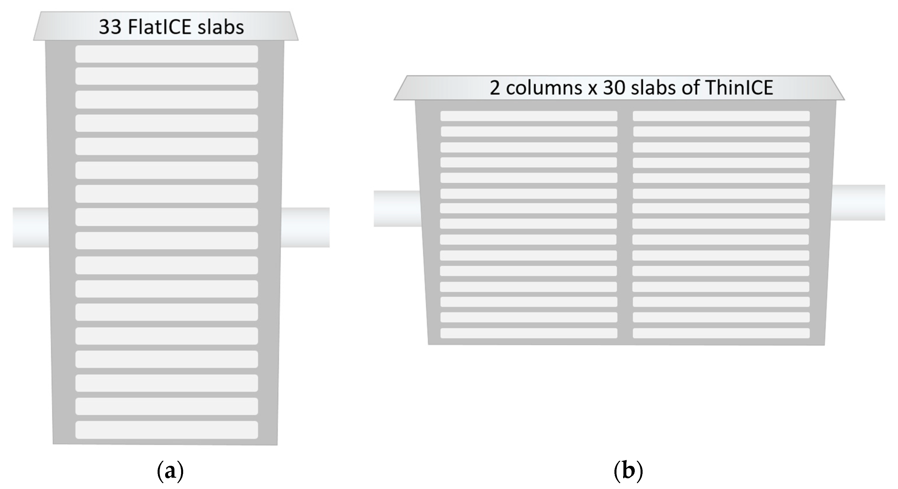
| Parameter | Flat-ICE | Thin-ICE |
|---|---|---|
| Length (mm) | 500 | 500 |
| Width (mm) | 250 | 250 |
| Thickness (mm) | 35 | 17 |
| Gap between slabs (mm) | 10 | 16 |
| Slab mass (kg) | 7.1 | 3.6 |
| Nº of slabs in optimization | 10 to 40 | 20 to 75 |
| Nº of columns in series in optimization | 1 to 3 | 1 to 3 |
| Parameter | Implicit Model | Explicit Model | ||||||||||
|---|---|---|---|---|---|---|---|---|---|---|---|---|
| Time-step (sec) | 10 | 1 | 10 | 10 | 10 | 10 | 1 | 1 | 1 | 1 | 1 | 1 |
| Nx (x-axis) | 25 | 25 | 25 | 15 | 15 | 5 | 5 | 25 | 25 | 15 | 15 | 5 |
| N_wall (y-axis) | 4 | 4 | 3 | 4 | 3 | 3 | 3 | 4 | 3 | 4 | 3 | 3 |
| N_PCM (y-axis) | 9 | 9 | 7 | 9 | 7 | 7 | 7 | 9 | 7 | 9 | 7 | 7 |
| MAPE(%) | Ref | 0.30 | 0.08 | 1.45 | 1.37 | 9.47 | 9.15 | 0.38 | 0.44 | 1.07 | 1.00 | 9.09 |
| Computing time (sec) | 427.7 | 1171.4 | 237.1 | 206.6 | 97.0 | 32.7 | 137.7 | 43.7 | 33.64 | 25.9 | 22.3 | 6.9 |
| (TIMExMAPE)/100 | Ref | 3.61 | 0.19 | 2.99 | 1.33 | 3.10 | 12.56 | 0.16 | 0.15 | 0.27 | 0.22 | 0.62 |
| Time percentage in the range 1–3 kW (%) | 56.8 | 56.8 | 56.6 | 56.9 | 56.8 | 57.4 | 57.4 | 56.9 | 56.7 | 57 | 56.8 | 57.4 |
Publisher’s Note: MDPI stays neutral with regard to jurisdictional claims in published maps and institutional affiliations. |
© 2021 by the authors. Licensee MDPI, Basel, Switzerland. This article is an open access article distributed under the terms and conditions of the Creative Commons Attribution (CC BY) license (https://creativecommons.org/licenses/by/4.0/).
Share and Cite
Crespo, A.; Zsembinszki, G.; Vérez, D.; Borri, E.; Fernández, C.; Cabeza, L.F.; de Gracia, A. Optimization of Design Variables of a Phase Change Material Storage Tank and Comparison of a 2D Implicit vs. 2D Explicit Model. Energies 2021, 14, 2605. https://doi.org/10.3390/en14092605
Crespo A, Zsembinszki G, Vérez D, Borri E, Fernández C, Cabeza LF, de Gracia A. Optimization of Design Variables of a Phase Change Material Storage Tank and Comparison of a 2D Implicit vs. 2D Explicit Model. Energies. 2021; 14(9):2605. https://doi.org/10.3390/en14092605
Chicago/Turabian StyleCrespo, Alicia, Gabriel Zsembinszki, David Vérez, Emiliano Borri, Cèsar Fernández, Luisa F. Cabeza, and Alvaro de Gracia. 2021. "Optimization of Design Variables of a Phase Change Material Storage Tank and Comparison of a 2D Implicit vs. 2D Explicit Model" Energies 14, no. 9: 2605. https://doi.org/10.3390/en14092605
APA StyleCrespo, A., Zsembinszki, G., Vérez, D., Borri, E., Fernández, C., Cabeza, L. F., & de Gracia, A. (2021). Optimization of Design Variables of a Phase Change Material Storage Tank and Comparison of a 2D Implicit vs. 2D Explicit Model. Energies, 14(9), 2605. https://doi.org/10.3390/en14092605