Abstract
Nowadays, based upon human needs and preferring perpetual types of energy, photovoltaic system (PV) is a suitable alternative and more frequently used in northern countries, which are recently more attracted by solar power. The new floating type of the structure is installed in the water bodies instead of land. One of the main elements in floating photovoltaic structures is the forces imposed on the panels. In the northern regions, the dominant load is considered to be ice interaction with the structure. This study aims at identifying the loads imposed on a floating PV structure located in the Łapino Reservoir on the Radunia River, which are produced by the wind action on the ice cover. The wind velocity varying between 10 and 26 m/s is implemented, and also the reduction of the pool level was studied. Wind direction plays an important role in the inclination and expansion of ice accumulation. Moreover, the magnitude of wind velocity is a determinative factor in the maximum thickness emerged in various spot of the area. Changes in pool level reduction is not able to cause noticeable changes in ice cover expansion and maximum ice thickness. Additionally, the shoving mechanism is able to originate abrupt changes in ice thickness by means of rising wind velocity.
1. Introduction
In the last decades, the earth has faced a new challenge in climate change, which is directly related to fossil fuel extraction and consumption. It leads mankind to rely on more renewable energy sources (RES), and the most important is the electricity segment [1]. In the past 10 years, RESs have an increase of about 8% per year in the power installation, which is mainly related to the photovoltaic installation sector with a growth rate of 45%. [2]. The system integrates existing land based photovoltaic technology with a newly developed floating photovoltaic technology on dams, reservoirs and other bodies [3]. Compared to ground based types of this structure, this can be of more benefit in terms of cost reduction, lowering water surface, regulation of temperature, land usage, etc. [4]. The floating photovoltaic system has been appreciated in many parts of the world; for instance, the United States, Italy and others [5].
There are different considerations in designing and installation of photovoltaic systems; environmental impacts like lightning strikes, high efficiency with power output and low energy demand in production, mechanical loads, etc. [6,7,8,9]. Installation of these structures needs to take into account different forces imposed by water flow, wind and ice effect, etc. at the installation zone that brings complexity to the work. As mentioned above, in cold regions, the ice load is the dominant force affecting the floating PV installations. Inland water ice processes include various types of integration concerning hydrodynamic, mechanical, and thermal actions [10]. During a river’s freeze-up period, depend on flow characteristics, ice may form on the calm water as skim ice or frazil ice in turbulent flow. Since the floating PV facility is typically installed on the water bodies characterized by the low flow velocity, it is commonly subjected to the static ice cover formation. During the winter months, the cover is influenced by weather and hydrologic conditions, from which the wind is the most important factor to be considered.
Horizontal forces of ice are categorized in static and dynamic forces. The static forces are applied due to the obstruction of the ice cover movement by the structure, and the dynamic forces are caused by the ice cover movement influences on the structure. Different parameters may lead to static forces in the ice-structure interaction: water level variation, drag forces created by wind and water layer beneath the ice cover, thermal changes, etc. [11].
The first step is to classify the reservoir area in terms of the ice formation process (static or dynamic ice cover). It will depend on the hydrodynamics and thermodynamics features, which in a nutshell leads to estimating whether the water in the tank will mix in its entire volume as a result of the flow, or whether the stratification equilibrium will be maintained [12,13]. In areas of low flow in the reservoirs, a considerable rate of water turbulence in the vertical direction does not occur to make it possible for cold water to be mixed with frazil ice. As a result, in the areas with this hydrodynamic feature, ice particles grow at the surface, and skim ice cover forms over the water surface. This cover expansion acts as an ice isolation layer to prohibit the water from dropping depth-averaged temperature below freezing. By continuing the concentration, ice pans may form on the surface [14]. Furthermore, the variation range for water velocity, discharge and air entrainment at the vicinity of the structure should be taken into account [15]. The importance of the water velocity and discharge in river ice is their effect on the progress of ice formation in the water body [16], which will define the type of forces imposed on structures. Moreover, since normally the surface ice can be under the effect of wind blowing [17,18], and evidence shows that the wind action may have a fundamental influence on river ice dynamic [19], the wind effect on ice structure interaction needs to be considered.
There are a number of studies in the past related to different type of forces caused by wind and water velocity, and ice formation on hydraulic structures like FPVs. Trapani and Millar [20] study aimed at minimizing the loads on the flexible structures with similar mooring arrangements to wave energy converters (WECs). Dai et al. [6] innovated a system to contain a number of standardized floating modules made of high density polyethylene (HDPE) that may serve as photovoltaic panel floaters. They applied hydro elastic simulation to the hydro-structural response of the floating system under the wave influence. Lee et al. [21] studied the effect of both wind and wave on floating PV structures. Wind direction appeared to affect only the front edge in front of the flow. Backward wind caused higher loads, drag than did the former one.
Kolerski et al. [22] altered a 2D hydro–ice dynamics interaction model for the ice-boom interaction with water currents and wind. The numerical simulation was a couple of hydrodynamic and ice dynamic models. Meyer and Coufal [23] surveyed hydraulic conditions of steady motion in an estuarial river section, and the analysis of swelling curve under wind influence. Kolerski et al. [24] studied the wind force on ice on the coast of a lagoon and the ice jam formation by means of DynaRICE modeling. Staneva et al. [25] studied the wind-wave interaction effects in a wave–ocean circulation model on Lagrangian transport simulations. Wake and Rummer Jr. [26] developed a previous thermodynamic model of ice formation and extended it to consider ice movement and deformation due to both wind and water interaction. Morse and Richard [27] investigates correlation of air and water temperature accounting wind surface ice thickness anchor ice thickness, etc. Shen et al. [28] formulated a one-dimensional river-ice simulation model RICEN, accounting wind effects on the ice-jam process and resistance of the flow due to the ice movement.
The aim of this study is to define the possibility of utilizing the reservoirs for installing the floating structures in Northern Europe. The floating PV structure installed on Łapino Reservoir is the first attempt to install the mentioned type of structures in northern countries. In the past studies, the effect of ice on these structures is not considered; therefore, this work aims at bringing a new quality to this area of expertise. Due to the hydrodynamic and thermodynamic condition imposed on the subjected area, the wind velocity impact on ice is the most influential factor to be considered in the determination of the loads impacting the structure. The study also sought to consider the wind effect on ice thickness variation on the reservoir domain. Needless to say, in the small area of the reservoir, the pool level may vary considerably. Therefore, in the case of maximum wind effect, another profound change in water level is considered.
2. Materials and Methods
2.1. Site Description
Energa OZE Inc is located in Gdańsk, Pomorskie, Poland and is part of the Electric Power Generation Industry. The company is planning to implement an innovative project of photovoltaic panels floating on water. This will be the first undertaking of this kind in Poland, and is yet another renewable energy project in the Energa Group. The floating photovoltaic panels on water would be installed on a reservoir in Łapino, municipality of Kolbudy. The Łapino reservoir on the Radunia River is a small reservoir with the single purpose of hydropower generation (Figure 1). Due to this specific function of the dam and the small area of the reservoir (0.37 km2), the water level varies by a noticeable range.
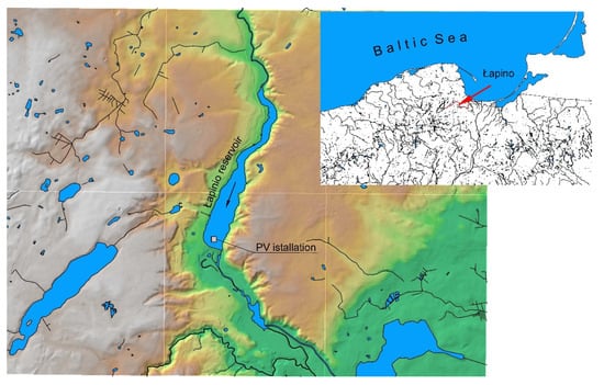
Figure 1.
Location of the PV installation on the Łapino Reservoir.
The impounded facility Łapino uses a dam to store the Radunia River water in the reservoir and released through the turbine, which leads to regular changes in the position of the water table, within the range of 99.8–98.2 m above sea level during the day. Despite such large daily fluctuations, the speed of water in the reservoir is very low. The performed numerical simulations showed that under the conditions of the maximum flow through the hydropower plant, Q = 22 m3/s, the water velocities in most of the reservoir area do not exceed Vw = 0.1 m/s (see Figure 2). This is due to the relatively large depth of water, up to 8 m in the lower part of the reservoir.
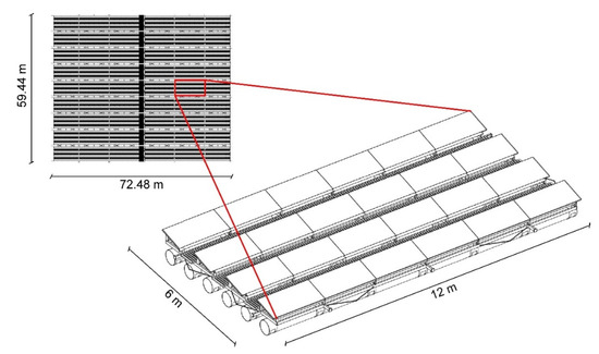
Figure 2.
Plane view and single module of PV installation.
The object of the photovoltaic power plant consists of floating platforms with anchoring elements and elements of equipment, photovoltaic panels with a substructure and power plant network equipment. The platform is designed to be floating, located approximately 55 m from the embankment of the reservoir. The platform in the projection has the shape of a rectangle with dimensions of 59.44 × 72.48 m, consists of 54 modules, tied up with dead anchors. The photovoltaic installation is designed for 4 types of rectangular elements with the dimension of 6 × 12 m (Figure 2). A connection between the modules allows free movement of the panels. Modules equipped with plastic floats with a diameter of 0.5 m and length of 12 m. On the floating platform, a supporting substructure has been designed for photovoltaic panels with a total power of 0.5 MW, including cabling and operating equipment.
2.2. Determination of the Characteristic Ice Thickness for the Łapino Reservoir
The experimental work of Hammar et al. [29] resulted in a certain range for skim ice. They showed that in slow flowing areas at the approximate range of 0–0.1 m/s, ice crystals formed on the supercooled water surface will remain on the surface to form a thin stationary or moving skim ice sheet. In the wide area of the reservoir, the water velocity is at the range of 0–0.05 m/s, and the negligible bounded area near the outlet related to the higher velocity is due to the 6 h per day of temporary water release, which seems not to make frazil ice formation due to being flushed away on the spillway. Therefore, it is expected to create a cover in the form of static skim ice on the entire reservoir, which will be generated at the beginning of the winter season as a result of density mixing and water stratification equilibrium [30].
Based on these data provided by the hydro power station (bathymetry and discharge), the water velocity is calculated for the whole domain. Based upon the calculated velocity, the low flow is observed in a wide area of the reservoir. In this low flow condition, the stationary skim ice will be formed. The process of ice formation in stagnant waters or waters flowing at a slow speed without causing turbulent mixing is associated with the traversing of the top layer of water. Due to the physical property of water, which reaches its maximum density at 4 °C, cooling the water will generate mixing until it reaches 4 °C. Further cooling of the water will not result in convective mixing, as the lighter layer of cooler water will lie on the surface of the warmer water. In such a situation, only the surface layer of water will be cooled, and it is supercooled relatively quickly (temperature slightly lower than 0 °C) and the formation of a permanent ice sheet (Shen 2010). The cover formed by the vertical water density stratification is uniform in thickness and has a smooth bottom surface [31]. The described phenomenon is characteristic for lakes and water reservoirs, as well as sections of rivers with a low flow velocity [28], such as the analyzed Łapino reservoir on the Radunia.
Modeling the thickness of the ice cover can be done based on a complete description of the phenomenon, thus obtaining very accurate ice conditions in the river. In order to use such a model, it will be necessary to take into account the hydraulic and meteorological data in the form of water speed and state, and the heat balance of the ice surface [16]. Additionally, it will be necessary to introduce data on the physical and mechanical properties of ice into the model. Obtaining such an amount of data is very difficult or even impossible in the case of the analyzed Łapino location.
In general, the process of increasing and decaying the thickness of the ice depends on the heat transfer on both the upper and lower surfaces of the ice. The temperature distribution over the thickness of the ice can be described in the form of the diffusion equation [32]. Solving this equation requires the calculation of the full heat balance on the water surface, which leads to the acquisition of great meteorological data, unavailable for the analyzed location. An alternative to the full mathematical model is ice thickness modeling using the cumulative average daily negative air temperature (freezing degree day, FDDs). Freezing degree-days (FDD) are correlated with natural phenomena such as thickness of lake ice, spring breakup of ice, and depth of frost in the ground [33]. This method is proposed as Stefan’s formula [34]. After further modifications by Michel [35], the method for calculating the increase and decay of the thickness of the ice sheet was presented in the final version in the work of Shen and Yapa [36]. The main advantage of the method presented here is its great simplicity in its application to practical issues, with relatively high compliance with the observations at the same time. The input data are only the air temperature, which is easy to obtain, both as historical data and in the form of a forecast.
The basic assumption of the method presented below is the linear distribution of temperature over the thickness of the ice sheet. If, in addition, no snow cover is assumed, then the thickness of the ice cover at a given time can be determined from the difference in temperature at the top and bottom thickness of the ice surface [17]:
where —heat flux passing through the ice [W·m−2] at time t, and denote the ice temperatures at the air-ice and ice-water interface [°C], respectively, ice thermal conductivity = 2.24 W∙m−1∙°C−1, while is the thickness of the ice cover [m] at time t. After taking into account the boundary conditions on the interface between water and ice, and ignoring the heat flux caused by the penetration of short-wave radiation, it is possible to present the change in the thickness of the ice cover with time in the form of an ordinary differential equation [37]:
in which is the air and water temperature, respectively [°C], —the melting point of ice [°C], is mass density of ice, and is the latent heat of melting ice [333,000 kJ·kg−1]. The heat flux supplied to the ice on air-ice plane is taken into account in the form of linear heat transfer coefficients, [W∙m−2∙°C−1]. Integrating the Equation (2) with a time step equal to one day leads to the formula for calculating the increase and decay in the thickness of the ice cover based on the sum of daily temperatures:
In the equation presented above, represents the initial thickness of the ice sheet [m], is the sum of average daily temperatures [°C].
The meteorological data including air temperature collected by Institute of Meteorology and Water Resources (IMWR) from Świbno station were used for the calculation. The station in Świbno is located about 30 km from the Łapino reservoir, and its elevation is about 100 m lower than the pool level of the reservoir. For this reason, in order to determine the consistency of the obtained results, the calculated ice thickness on the basis of the Świbno station was compared with a single measurement of air temperature from the meteorological station located in close distance (Szadółki station). The FDD method is used for the calibration. The comparison of data from the 2016/2017 winter season shows that the maximum computed thickness of ice for Świbno and Szadółki station are 12.05 and 12.37 cm respectively (Figure 3). The estimated error of the calculated thickness for Świbno station is 2.5%, which is acceptable. Since the data for Szadółki station, which is the closest station, are only available for 1 season, the data from Świbno station can be used for the whole simulation (see Figure 4).
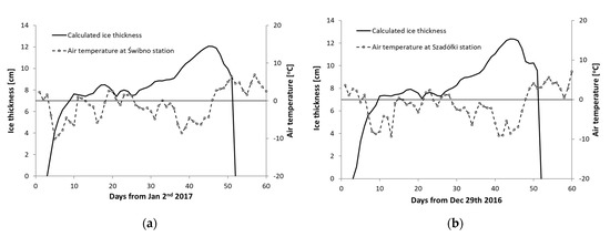
Figure 3.
Calculated thickness of the ice cover on the Łapino reservoir in the winter season 2016/2017 based on the sum of negative temperatures of the IMWM station in (a) Świbno and (b) Szadółki.
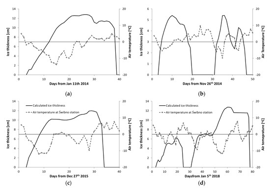
Figure 4.
Calculated thickness of the ice cover on the Łapino reservoir in 2013-2019 based on the sum of negative temperatures from the Świbno station in the winter season (a) 2013/2016; (b) 2014/2015, (c) 2015/2016 (d) 2017/2018.
The table below (Table 1) summarizes the results of calculations in the form of the date of ice start and breakdown and the date of maximum ice thickness in each winter season. The charts show the air temperature data, as well as the result of the increase and loss of ice thickness in the reservoir in individual seasons. For performing a more conservative calculation (the ice thickness observed for Szadółki is higher than Świbno station), the thickness of 15 cm has been used for the calculation.

Table 1.
Results of ice thickness calculations on the Łapino reservoir in 2013–2019.
2.3. Wind Speed and Direction
Ice can affect hydraulic structures in three ways:
- Dynamic impact of flowing ice floes against the structure [38]
- Static pressure due to constrained thermal expansion of ice [39]
- Static pressure of wind and currents on the structure [40]
Due to the existing hydrodynamic conditions (deep reservoir with low inflow), water drag will be negligible. To eliminate potential static pressure on the ice sheet due to thermal expansion, an open water space should be maintained between the structure and the ice sheet. The installation will only be subjected to static forces from the ice sheet, which will be pushed by the wind [41].
Wind data have been provided for the study covers the years 2015–2019, recorded 3 times a day at 6:00, 12:00 and 18:00 o’clock. They come from the Institute of Meteorology and Water Management and are interpolated from the nearest observation stations to the location of the Łapino reservoir. For this reason, it should be presumed that the wind direction does not take into account the local topography of the area and does not relate precisely to the situation that actually takes place over the valley of the Radunia River. The data were analyzed in terms of the frequency of the phenomenon throughout the observation period, the winter season of 2015−2019, and in individual months in that specific period. The wind data are shown in the Table 2. The following were assumed for the calculations:
Table 2.
The frequency of wind occurrence distributed over cardinal directions for the winter months in 2016–2019.
- (a)
- Maximum wind from the observation at 15 m/s from the north
- (b)
- As an abnormal wind (wind gust) the speed of 20 m/s, blowing from the north
- (c)
- Design wind with a speed of 26 m/s blowing from the north considering the climate change concept.
In all cases, it was assumed that the west direction, which is dominant in the measurement data, is not correct due to the high left bank of the reservoir. For this reason, it was assumed that the design direction used in further calculations will be the north (N) and north-north-east (NNE) direction, i.e., along the river valley and in the direction of the water flow (Figure 1). At the same time, it will be the least favorable direction due to the location of the planned installation in the downstream part of the reservoir. In the event of a northward wind, the ice field pressing against the edge of the structure will extend for a distance of about 1000 m, thus generating the greatest forces on the structure.
2.4. Mathematical Model
2.4.1. Applied Equations on Ice Dynamics
As mentioned above, ice processes are influenced by hydrodynamics, thermodynamics and the ice mechanics. In order to grasp the full picture of the phenomena taking place, it is necessary to derive an equation presenting the balance of forces acting on the ice. The equation of the balance of internal and external forces acting on a fragment of the ice rubble floating on the water surface can be presented in the form of the momentum conservation equation (Newton’s second law of dynamics) [42]
where is the unit mass (on the surface) of the ice particle under consideration, [m·s−1] is the ice velocity vector, is the acceleration of ice moving on the water surface, is the force resulting from internal ice stresses, is a force related to the effect of wind on ice, is the force representing the water drag on the underside of the ice cover, and is the force of gravity. and are the normal components of the internal stress in ice rubble, while are the tangential components of the internal stress of the ice. All stresses are determined at the point where the considered ice particle is located. The location of this point is described in the form of a vector , which is defined as follows: . and are surface ice concentration and ice thickness, respectively. Parameter Cw [–] is the wind interaction factor, Cw = 0.00155 [43], and are the air and water density respectively [kg·m−3], [m·s−1] is the velocity of water, [m·s−1] is the speed of wind at a height of 10 m above the river surface, is the coefficient of roughness of the underside surface of the ice, [m] is the water depth under the ice cover, while [–] is a parameter describing the proportion of the active cross-sectional area under the influence of the impact of ice.
2.4.2. Static Ice Pressure on the Structure
Assuming the buoyancy of the ice sheet, its thrust on the structure can be determined from the balance of forces presented below. Forces acting in the x and y directions are determined from the following equations [42,44]:
where X and Y are components of the ice barrier reaction, and are the components of the water drag in x- and y- directions, respectively, and are the components of the wind drag in x- and y- directions, respectively. Determining X and Y from the above equations, and ignoring the higher-order terms, the normal and tangential stresses acting on a segment of a differential length dl can be determined:
According to the preliminary assumption, the ice cover with a uniform thickness of 15 cm was set over the entire calculation area, except for the squared space delineating the planned PV installation. Full freedom of ice movement was assumed, which means that the particles representing the ice cover can both move vertically with the changing water level and also have the ability to move horizontally. The movement of ice in the horizontal direction is a consequence of the dynamic balance of external forces acting on the ice (see Equation (4)). From the forces presented here, both the force of gravity and the force of flowing water will be of negligible importance, due to the practically horizontal arrangement of the pool water level in the reservoir and the negligible speed of water flow. The displacement of the ice will be mainly caused by the force from the wind and the drag force due to stresses inside the ice. The dynamic balance of these two forces will result in ice movement within the area.
The forces transmitted through the ice are recorded on the perimeter of the planned structure at intervals of approximately 15 m (five points on each edge). The value is given in kN/m, i.e., the total force must be multiplied by the length of the structure segment.
2.5. Model Implementation
The calculations were performed for the water inflow to the reservoir from the Radunia river, Qin = 22 m3/s. Initial water level was set at the normal pool level H = 99.6 m (set at the weir of the Łapino dam). Outflow from the reservoir through the hydroelectric power plant was equal to inflow Qout = 22 m3/s. At the beginning of each simulation, ice covers the entire surface of the lake with a thickness of η = 0.15 m. North wind speed varying from 10 to 26 m/s was used, and the velocity remains constant for 12 h of each simulation. The model was implemented in the reach of approximately 1100 m long, covering 26 ha of the area (70% of the total area of the reservoir).
A network of triangular finite elements with variable linear dimensions was built in this area. In the immediate vicinity of the PV installation, the elements have a linear dimension of 6 m, and then increase to 15 m in the upper part of the reservoir. In the area of the inlet to the hydroelectric power plant and the spillway, the elements have a linear dimension of 3 m in order to adequately address the boundary condition. Finally, the model consists of 5215 nodes and 10,032 elements, as shown in Figure 5c.
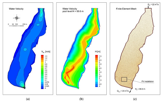
Figure 5.
Results of numerical simulations conducted on the Łapino reservoir, Q = 22 m3/s and the pool level H0 = 99.6 m (a) water velocity, (b) water depth (c) finite element mesh for the area from the Łapino reservoir; the figure shows the locations of open boundary conditions-flow and water level.
The open boundary conditions were set in such a way as to reflect the actual conditions of water flow through the Łapino Barrage as much as possible. On the upper open boundary, a constant inflow of Qin = 22 m3/s was applied, identical to the outflow, which was discharged at the inlet to the hydroelectric power plant. It was assumed that during the water discharge, the weir will not be open, but the water level will be maintained at the initial value of 99.6 m above sea level (water level recorded during the bathymetric measurement on 14 September 2019). Then, over the next 12 h, the water level will decrease linearly to the final elevation of 98.6 m above sea level (lowering the damming level by 1 m). This procedure is in line with the half-day equalization hydroelectric mode, which is also confirmed by the observation data of the water level on the reservoir. As the water discharge often caused a decrease in water by 2 m, calculations were also carried out for these conditions, i.e., lowering the water table to the ordinate of 97.6 m. The locations of the open boundary conditions are shown in Figure 5c.
3. Results and Discussion
The results are presented in Figure 6 and Figure 7 the form of contour charts of the thickness of the ice on the reservoir -and Figure 8 the distribution of normal and tan-gential forces on the contour of the planned installation. Additionally, the size of the calculated force is shown in the table (Table 3).
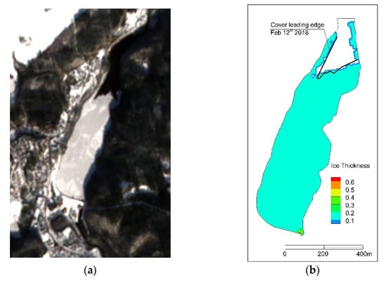
Figure 6.
Comparison of the (a) satellite image of 12 Feb 2018. Sentinel-2. (b) Results of the numerical simulation, ice distribution in the Łapino reservoir under the conditions of the north wind with a speed of 13 m/s (high wind).
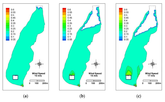
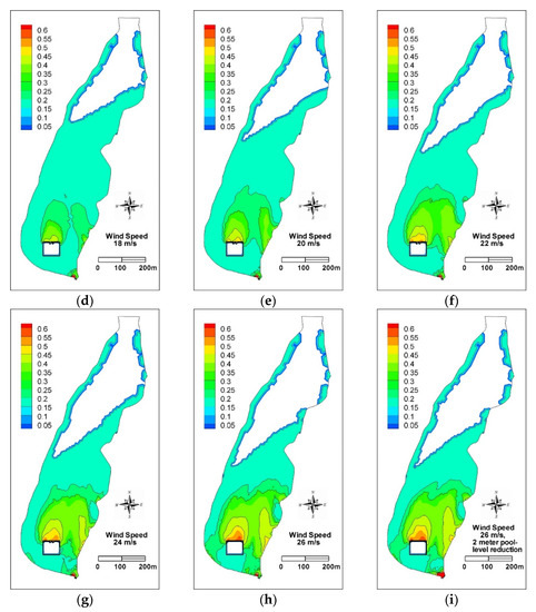
Figure 7.
Ice thickness expansion on the reservoir surface domain at different northerly wind speed, and (a–h) for lowering the damming level by 1 m and (i) for reduction of the pool level by 2 m.
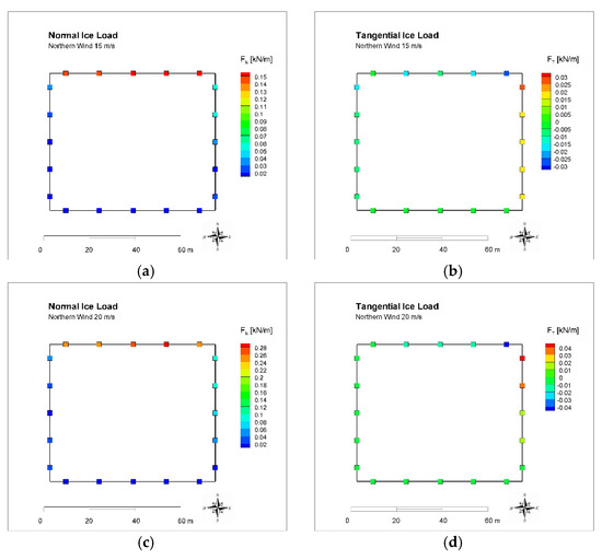
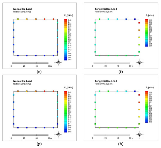
Figure 8.
Normal and tangential ice load per meter imposed on structure edges based upon different wind velocities; shapes (a–f) represents numbers for 1 m, and (g,h) 2 m pool level reduction.
Table 3.
Forces resulting from static ice pressure on the PV installation in the conditions of the northern wind with variable speed.
As it is not possible to calibrate the model due to the lack of observation of ice phenomena on the Łapino reservoir, the area occupied by the ice obtained from the calculations was compared with the satellite image taken on 12 February 2018 (Figure 6), obtaining a high agreement of the results. Considering ice movement in both figures, the upstream part shows to be free of ice. As regards both figures, at the high velocity of 15 m/s, and due to the structure existence, the ice can be accumulated at the upstream edge of the structure.
Figure 7 illustrates the expansion of ice under the northern wind. It is needed to consider that wind blowing from the northern side plays an act in pushing the ice and making it more compact at the adjacent of the structure layout. Considerable changes in the ice thickness at the southern part of the domain are not the subject of analysis, since these changes are based on the lowering the pool level, and the water in this area will pass through the spillway. Apart from the bank, the structure edges themself play a role as borders on the stream direction, therefore bridging the ice near the borders leads to thickening the primary ice cover and forming the secondary ice layer. At the bottom of the wind speed variation range, 10 m/s does not cause many changes on the primary ice thickness. By increasing the speed to 15 m/s, more noticeable changes start to happen. At this mentioned speed, the changes are observed more in front of the northern edge of the structure and less at the vicinity of the bank.
Growing to 20 m/s, the ice expansion near the bank and the structure unify to create a more expanded domain. Regarding 22 m/s, the larger thickness ice expanded area gradually extends to the north direction, and also two other increasing border ice spots can be recognized. Furthermore, ice compaction both at the border edge of the structure and the bank rises by around 0.05 m. However, during the whole trend, more compression is observed adjacent to the structure. Rising to 26 m/s, the new spots of border ice unify with the extended area of the ice compaction, and the whole area extends both to the north and south direction. Moreover, at this case of 26 m/s of wind velocity, expansion of greater ice thickness is observed at the south-western domain. Considering the overall trend, the most ice contraction is located first at the upstream edge of the structure, and then near the bank. Moreover, by increasing the wind speed, the free of ice surface area increases due to the impaction of the ice particles to the south. Needless to say, stream direction is at south-east direction, hence the ice thickness changes are generally more observed in this direction. A 2 m pool level reduction does not make a noticeable difference with 1 m, for 26 m/s wind speed. Since the former pool level reduction is the worst-case scenario, it can be concluded that water level changes may not affect the ice thickness compaction to a great extent. Although, at the former case, more contraction is noticed near the bank and the structure.
Figure 8 illustrates the number for different loads (both normal and tangential) exerted on different nodes located on the edges of the structure border. Considering the normal forces, the left side of the northern edge bears the maximum loads. The largest normal load imposed on the structure at the case of 1 m reduction damming level and 26 m/s is 1.43 and 2.7 times that of 20 and 15 m/s, respectively. Practically, negligible minimum normal forces are imposed on the bottom edge. On the corner edges (western and eastern), the left one is under the minimum normal tension, apart from the northern part of the left edge, which is placed under a slightly higher normal load. Northern part of the right edge is relatively under higher normal forces in comparison with the left edge; the difference exceeds by increasing the wind velocity (the maximum amount for the right edge is 0.05, 1.67 and 2 times that of the left edge for 15, 20 and 26 m/s of wind speed, respectively). A 2 m reduction of damming level does not make noticeable changes on exerted normal forces, although it makes the maximum normal force in the right edge to expand to a larger part of the edge, and a slight increase in the northern section of the left edge.
Tangential force distribution on the north edge shows that the maximum load accrues on the right side at the left direction. This maximum amount in 26 m/s sample is 2.67 and 1.6 times the amount of 20 and 15 m/s of wind velocity cases, respectively. Considering ice contraction and the trend of tangential load on this mentioned edge implies that the separate area of maximum ice jamming may cause the fluctuation force imposing trend. As regards the southern edge, tangential loads show insignificant amounts. The evident reason is the safe zone for this edge based on the direction of the wind. At both corner edges, the tangential force is in south direction, with the maximum amount located on top of both edges. It is also considered that a 2 m damming level reduction may not change the range of the tangential load to a great extent. However, it changes the maximum amount of tangential load on the left edge to 6 times the 1 m type.
Table 3 indicates the numbers for both normal and tangential forces placed on different edges of the structure. Figure 9 demonstrates the magnitude and direction of the force vectors placed on the structure edges for 26 m/s wind velocity. Regarding Table 3, it can be concluded that in the case of wind speed of 26 m/s, there is more fluctuation in the force magnitude on different edges, and by decreasing the wind velocity, more equipoise in the imposed forces is observed. Furthermore, roughly zero amount for the tangential forces imposed on the southern edge in variety of wind velocity shows approximately no impact of the wind on this edge. This is due to the fact that, because of the wind action, the contact between this edge of the structure and ice cover has been reduced. Although, there is not a large space between the ice cover and the southern edge, and there still is a slight contact between the edge and the ice cover. Considering both the table and figure, tangential forces are mostly seen in the western direction for the northern edge, and the southern direction for the eastern edge. Regarding the fact that both the other western and southern edges do not bear noticeable total forces, a tilting at the south-east direction is predicted. The tilting direction of the structure is more or less the same for different wind speed and pool level variation.
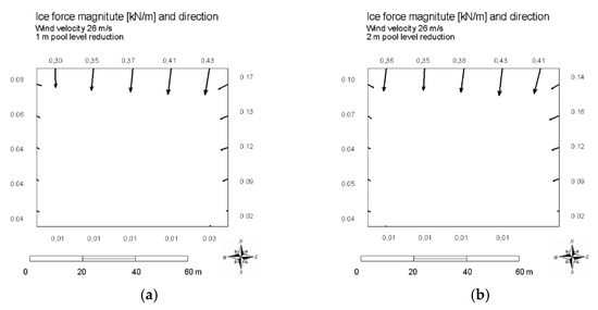
Figure 9.
Magnitude and direction of the force vectors placed on the structure edges for (a) 26 m/s wind velocity with 1 m and (b) 2 m pool level reduction.
There are not many former studies related to ice load on photovoltaic structures, especially when the wind action is issued. Although, the approach that has been taken was also applied for other floating subjects. One of the case studies with the same approaches is numerical simulation of ice transport over the lake Erie-Niagara River ice boom [43]. The resulting loads in the mentioned study are not comparable to this current one; since the length of the water body and wind velocity in the worst-case scenario (this condition is considered for the imposed forces calculation) are in a larger scale (200 km and 50 m/s, respectively). Furthermore, in this case study, only the real case scenario is contemplated for exerted forces calculation; therefore, no wind action scenario has been taken into account as a comparison. The other study conducted based upon a similar approach is implementing a DynaRICE model for the treatment of ice-boom interaction with the effect of wind and tidal current due to the more closeness with the scale of the lake and wind velocity (5 km and 25 m/s, respectively), maximum calculated loads on the structure coincides with this present study.
Figure 10 indicates the maximum normal and tangential forces imposed on the structure for the variety of wind speed. Normal force shows a wider range of variation, in comparison with tangential force. The variation range for normal force shows to be 5.8 times that of tangential force. From 10 to 20 (m/s), a steep increase is observed in maximum normal force (from 0.07 to 0.31 kN/m). From 22 to 24 m/s, a less sharp increase in normal load is observed, followed by another sharp increase to 26 m/s (0.42 kN/m). As regards tangential load, no linear trend is observed. Between 10 and 13, 18 and 20, and 25 and 26 m/s, no noticeable change in maximum tangential load is observed, which are generally followed by a steep change in maximum load. This abrupt change is more observed between 20 and 22 m/s (0.05 to 0.07 kN/m), which is before occurring an immediate reduction in maximum force (0.06 kN/m). Basically, from 21 to 24 m/s, a downward trend is observed in maximum tangential loads.
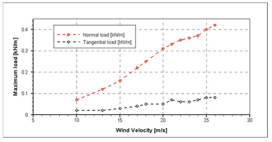
Figure 10.
Maximum normal and tangential load imposed on the structure for the variety of wind speed.
Figure 11 represents the expansion of ice and the location distance of double thickness and triple thickness to the structure. It should be noted that the structure is located at roughly 1200 m distance from the upstream open boundary of the domain. At the range of less than 10 m/s of wind velocity, there is not noticeable change in ice cover expansion. After applying 10 m/s, wind shifts ice cover abruptly, and a sudden shrinkage happens to 1070 m. Reaching 13 m/s, another steep contraction is shown to 800 m. Between 17 and 21 m/s, ice cover slightly varies from 800 to 700 m. From 21 to 23 m/s, another sharp shrinkage in the ice expansion is observed to 650 m. Between 23 and 25 not any noticeable decline occurs, and from 25 m/s another immediate shrinkage starts.
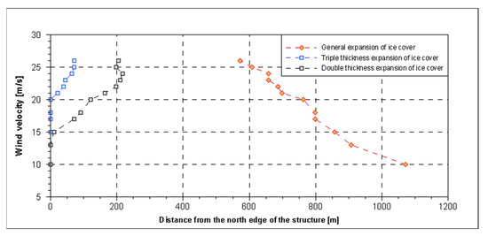
Figure 11.
Expansion of ice and the location distance of double thickness and triple thickness to the structure.
Double thickness of ice cover location indicates the power of wind to contract the ice cover. The farther from the structure it is, the more powerful the wind act on ice shrinking. At the rage of less than 13 m/s, no double ice thickness is observed; after 13 to 15 m/s, it appears at the instant vicinity of the structure. From 15 to 17, it recedes abruptly to 71 m of the structure, due to the mentioned ice shifting by the wind. Between 17 and 21 m a slight curved increment to the distance takes place (to 164 m). From 22 to 24 m/s, a mild linear increment in the distance happens, which is followed by a reduction in the distance in 25 and 26 m/s.
Based on the aforementioned numerical results, it can be concluded that mechanical ice cover thickening is represented by the model. The reservoir domain in this study can be referred as a wide river, which is a basic for mechanical thickening, so called “Shoving mechanism” [35,44]. Mechanical thickening is resultant of stream-wise direction force growth. By means of growing this mentioned force, which in this study is supposed to be wind action, the ice accumulation stress will overcome the internal resistance of the ice, therefore the accumulation emerges and continues until an equipoised ice thickening occurs.
4. Conclusions
This study aims at designing the loads imposed on the planned floating PV structure on the Łapino reservoir. Due to the very low flow velocity in the reservoir and thermal expansion space consideration into the designed structure, the only considerable force on the planned structure will be the static pressure of the floating ice sheet pushed onto the structure by the wind. A series of numerical simulations were carried out using the DynaRICE mathematical model. Due to the low flow dynamics in the winter season, a relatively smooth and uniform ice cover on the surface is formed, which is determined to be 15 cm, applying the freezing degree day (FDD) method for this study. As a result of high banks of the reservoir (especially the left bank), it should be expected that the wind will be heading along the river valley from the north or south. For this reason, the north wind was used in the calculations. For the purpose of calibration, calculated ice cover on the reservoir was compared with the ice cover recorded on the satellite image taken in winter 2018. The obtained results are very consistent with the actual image. By means of implementing the model and conducting simulations, the most important results are as followed:
Wind direction plays an important role in the inclination and expansion of secondary ice layer formation. Moreover, the magnitude of wind velocity is a determinative factor in the maximum thickness emerged in various spot of the area; in such a way that by increasing the wind speed, maximum ice thickness noticeably rises. The main section of secondary ice layer is at the vicinity of the northern edge of the structure; although, by growth in wind velocity, scattered spots of this layer appear. Then, this scattered spots unify following the wind velocity increment. Moreover, changes in pool level reduction is not able to cause noticeable changes in ice cover expansion and maximum ice thickness. Additionally, shoving mechanism is able to originate abrupt changes in ice thickness by means of rising wind velocity.
As regards the impact of normal forces on structure edges, the largest normal load is imposed on the left side of the northern edge. In addition, negligible forces are imposed on the southern edge in different velocity. It can be concluded that for designing edges for imposed forces, the southern edge is possible to be assembled in this way to bear minor loads. Regarding the western and eastern edges, these undergo higher forces, and the northern section of both edges carry higher loads in comparison with the southern sections. In addition, 2 m reduction of damming level does not make noticeable changes on exerted normal forces. Needless to say, normal force shows a wider range of variation, in comparison with tangential force.
Considering tangential force distribution on the north edge, the maximum load accrues on the right side at the left direction. On the northern edge, a separate area of maximum ice jamming may cause the fluctuation loading trend. As regards the southern edge, tangential loads show insignificant amounts due to the safe zone for this edge as a result of wind direction. At both corner edges, the tangential force is in south direction, with the maximum amount located on top of both edges. The only noticeable change generated by 2 m pool level reduction is in the maximum amount of tangential load on the left edge to 6 times the 1 m type.
It can be conducted that in the case of wind speed of 26 m/s, there is more fluctuation in the force magnitude on different edges, and by decreasing the wind velocity, the edges seem to be more balanced in the matter of imposed forces. Tangential forces are mostly seen in the western direction for the northern edge, and the southern direction for the eastern edge. Furthermore, roughly zero amount for the tangential forces imposed on the southern edge in variety of wind velocity can be due to the fact that, as a result of the wind action, the contact between this edge of the structure and ice cover is declined. Also, since both western and southern edges do not bear noticeable total forces, a tilting at the south-east direction is predicted. The rotations of the structure based on the ice load can be considered in designing of the structure.
Considering the loads imposed on the structure, to remove possible static pressure of the ice sheet resultant from thermal expansion, an open water space is recommended to be designed between the structure and the ice sheet. There are a number of possible solutions, including air curtains, which drag warmer water to the surface, preventing the ice from freezing to the structure.
Due to the shoving mechanism, ice accumulation at the vicinity of the structure edges increases. The more ice accumulation emerges, the more pressure is imposed on the edges. Therefore, installation of ice control structures (i.e., ice booms) upstream of FPVs could be considered.
Based on this study, a few suggestions can be made as new parameters for the future studies. For instance, the effect of the shape of the floating photovoltaic structures on the pattern of ice accumulation can be an issue to be considered. In addition, the effect of ice retention structures on the imposed loads on the floating photovoltaic structures can also be a matter of attention. Furthermore, continuing the analysis of how much ice will form directly on the photovoltaic panels on the floating installation and how it will affect the stress of the supporting structure is also recommended for consideration.
Author Contributions
Conceptualization, T.K.; methodology, T.K.; software, T.K.; validation, T.K., and D.G.; formal analysis, T.K.; data curation, D.G.; writing—original draft preparation, P.R.; writing—review and editing, T.K.; visualization, T.K. and P.R.; supervision, T.K. All authors have read and agreed to the published version of the manuscript.
Funding
This research was funded by Energa Invest Ltd. (Gdańsk, Poland).
Institutional Review Board Statement
Not applicable.
Informed Consent Statement
Not applicable.
Data Availability Statement
All the data is provided by Energa Invest Ltd, in this study.
Acknowledgments
The authors express their gratitude to Jan Haftka, and Michał Kąkol from Energa Invest Ltd., for support and assistance in the preparation of the project and the materials provided.
Conflicts of Interest
The authors declare no conflict of interest.
References
- Cazzaniga, R.; Rosa-Clot, M. The Booming of Floating PV. Sol. Energy 2020. [Google Scholar] [CrossRef]
- Rosa-Clot, M. Floating PV Plants; Academic Press: Cambridge, MA, USA, 2020; ISBN 0-12-817061-1. [Google Scholar]
- Choi, Y.-K.; Lee, Y.-G. A Study on Development of Rotary Structure for Tracking-Type Floating Photovoltaic System. Int. J. Precis. Eng. Manuf. 2014, 15, 2453–2460. [Google Scholar] [CrossRef]
- Zhou, Y.; Chang, F.-J.; Chang, L.-C.; Lee, W.-D.; Huang, A.; Xu, C.-Y.; Guo, S. An Advanced Complementary Scheme of Floating Photovoltaic and Hydropower Generation Flourishing Water-Food-Energy Nexus Synergies. Appl. Energy 2020, 275, 115389. [Google Scholar] [CrossRef]
- Ranjbaran, P.; Yousefi, H.; Gharehpetian, G.; Astaraei, F.R. A Review on Floating Photovoltaic (FPV) Power Generation Units. Renew. Sustain. Energy Rev. 2019, 110, 332–347. [Google Scholar] [CrossRef]
- Dai, J.; Zhang, C.; Lim, H.V.; Ang, K.K.; Qian, X.; Wong, J.L.H.; Tan, S.T.; Wang, C.L. Design and Construction of Floating Modular Photovoltaic System for Water Reservoirs. Energy 2020, 191, 116549. [Google Scholar] [CrossRef]
- Hassaine, L.; OLias, E.; Quintero, J.; Salas, V. Overview of Power Inverter Topologies and Control Structures for Grid Connected Photovoltaic Systems. Renew. Sustain. Energy Rev. 2014, 30, 796–807. [Google Scholar] [CrossRef]
- Aßmus, M.; Bergmann, S.; Eisenträger, J.; Naumenko, K.; Altenbach, H. Consideration of Non-Uniform and Non-Orthogonal Mechanical Loads for Structural Analysis of Photovoltaic Composite Structures. In Mechanics for Materials and Technologies; Springer: Berlin/Heidelberg, Germany, 2017; pp. 73–122. [Google Scholar]
- Meitzner, R.; Schubert, U.S.; Hoppe, H. Agrivoltaics—The Perfect Fit for the Future of Organic Photovoltaics. Adv. Energy Mater. 2021, 11, 2002551. [Google Scholar] [CrossRef]
- Shen, H.T. River Ice Processes. In Advances in Water Resources Management; Handbook of Environmental Engineering; Springer: Cham, Germany, 2016; pp. 483–530. ISBN 978-3-319-22923-2. [Google Scholar]
- Carter, D.; Sodhi, D.; Stander, E.; Caron, O.; Quach, T. Ice Thrust in Reservoirs. J. Cold Reg. Eng. 1998, 12, 169–183. [Google Scholar] [CrossRef]
- De Woul, M.; Hock, R.; Braun, M.; Thorsteinsson, T.; Jóhannesson, T.; Halldórsdóttir, S. Firn Layer Impact on Glacial Runoff: A Case Study at Hofsjökull, Iceland. Hydrol. Process. Int. J. 2006, 20, 2171–2185. [Google Scholar] [CrossRef]
- Leppäranta, M. Freezing of Lakes and the Evolution of Their Ice Cover; Springer Science & Business Media: Berlin/Heidelberg, Germany, 2014; ISBN 3-642-29081-7. [Google Scholar]
- Lal, A.W.; Shen, H.T. Mathematical Model for River Ice Processes. J. Hydraul. Eng. 1991, 117, 851–867. [Google Scholar] [CrossRef]
- Dargahi, B. Flow Characteristics of Bottom Outlets with Moving Gates. J. Hydraul. Res. 2010, 48, 476–482. [Google Scholar] [CrossRef]
- Shen, H.T. Mathematical Modeling of River Ice Processes. Cold Reg. Sci. Technol. 2010, 62, 3–13. [Google Scholar] [CrossRef]
- Ashton, G.D. River and Lake Ice Engineering; Water Resources Publication: Littleton, CO, USA, 1986; ISBN 0-918334-59-4. [Google Scholar]
- Shen, H.T.; Su, J.; Liu, L. SPH Simulation of River Ice Dynamics. J. Comput. Phys. 2000, 165, 752–770. [Google Scholar] [CrossRef]
- Kołodko, J.; Jackowski, B. Ice Floods Caused by Wind Action. In Channels and Channel Control Structures; Springer: Berlin/Heidelberg, Germany, 1984; pp. 439–444. [Google Scholar]
- Trapani, K.; Millar, D.L. The Thin Film Flexible Floating PV (T3F-PV) Array: The Concept and Development of the Prototype. Renew. Energy 2014, 71, 43–50. [Google Scholar] [CrossRef]
- Lee, G.-H.; Choi, J.-W.; Seo, J.-H.; Ha, H. Comparative Study of Effect of Wind and Wave Load on Floating PV: Computational Simulation and Design Method. J. Korean Soc. Manuf. Process Eng. 2019, 18, 9–17. [Google Scholar] [CrossRef]
- Kolerski, T.; Shen, H.T.; Kioka, S. A Numerical Model Study on Ice Boom in a Coastal Lake. J. Coast. Res. 2013, 291, 177–186. [Google Scholar] [CrossRef]
- Meyer, Z.; Coufal, R. Hydraulic Conditions of Steady Motion in an Estuarial River Section under Wind Influence. Arch. Hydro-Eng. Environ. Mech. 2001, 48, 59–83. [Google Scholar]
- Kolerski, T.; Zima, P.; Szydłowski, M. Mathematical Modeling of Ice Thrusting on the Shore of the Vistula Lagoon (Baltic Sea) and the Proposed Artificial Island. Water 2019, 11, 2297. [Google Scholar] [CrossRef]
- Staneva, J.; Ricker, M.; Carrasco Alvarez, R.; Breivik, Ø.; Schrum, C. Effects of Wave-Induced Processes in a Coupled Wave–Ocean Model on Particle Transport Simulations. Water 2021, 13, 415. [Google Scholar] [CrossRef]
- Wake, A.; Rumer Jr, R.R. Great Lakes Ice Dynamics Simulation. J. Waterw. Port Coast. Ocean Eng. 1983, 109, 86–102. [Google Scholar] [CrossRef]
- Morse, B.; Richard, M. A Field Study of Suspended Frazil Ice Particles. Cold Reg. Sci. Technol. 2009, 55, 86–102. [Google Scholar] [CrossRef]
- Shen, H.T.; Wang, D.S.; Lal, A.W. Numerical Simulation of River Ice Processes. J. Cold Reg. Eng. 1995, 9, 107–118. [Google Scholar] [CrossRef]
- Hammar, L.; Shen, H.; Evers, K.; Kolerski, T.; Yuan, Y.; Sobczak, L. A Laboratory Study on Freeze up Ice Runs in River Channels. In Ice in the Environment, Proceedings of the 16th IAHR International Symposium on Ice, Dunedin, New Zealand, 2–6 December 2002; International Association of Hydraulic Engineering and Research: Dunedin, New Zealand, 2002; Volume 3, pp. 36–39. [Google Scholar]
- Li, N.; Tuo, Y.; Deng, Y.; An, R.; Li, J.; Liang, R. Modeling of Thermodynamics of Ice and Water in Seasonal Ice-Covered Reservoir. J. Hydrodyn. 2018, 30, 267–275. [Google Scholar] [CrossRef]
- Ashton, G.D.; Kennedy, J.F. Ripples on Underside of River Ice Covers. J. Hydraul. Div. 1972, 98, 1603–1624. [Google Scholar] [CrossRef]
- Shen, H.T.; Chiang, L.-A. Simulation of Growth and Decay of River Ice Cover. J. Hydraul. Eng. 1984, 110, 958–971. [Google Scholar] [CrossRef]
- Schmidlin, T.W.; Dethier, B.E. Freezing Degree-Days in New York State. Cold Reg. Sci. Technol. 1985, 11, 37–43. [Google Scholar] [CrossRef]
- Stefan, J. Über Die Theorie Der Eisbildung, Insbesondere Über Die Eisbildung Im Polarmeere. Ann. Phys. Chem. 1891, 42, 269–286. [Google Scholar] [CrossRef]
- Michel, B. Winter Regime of Rivers and Lakes. Cold Regions Science and Engineering Monograph III-Bla; US Army: Hanover, NH, USA, 1971. [Google Scholar]
- Shen, H.T.; Yapa, P.D. A Unified Degree-Day Method for River Ice Cover Thickness Simulation. Can. J. Civ. Eng. 1985, 12, 54–62. [Google Scholar] [CrossRef]
- Ashton, G.D. River and Lake Ice Thickening, Thinning, and Snow Ice Formation. Cold Reg. Sci. Technol. 2011, 68, 3–19. [Google Scholar] [CrossRef]
- Tuhkuri, J.; Polojärvi, A. A Review of Discrete Element Simulation of Ice–Structure Interaction. Philos. Trans. R. Soc. Math. Phys. Eng. Sci. 2018, 376, 20170335. [Google Scholar] [CrossRef] [PubMed]
- Staroszczyk, R. On Maximum Forces Exerted by Floating Ice on a Structure Due to Constrained Thermal Expansion of Ice. Mar. Struct. 2021, 75, 102884. [Google Scholar] [CrossRef]
- Kärnä, T.; Kamesaki, K.; Tsukuda, H. A Numerical Model for Dynamic Ice–Structure Interaction. Comput. Struct. 1999, 72, 645–658. [Google Scholar] [CrossRef]
- Wu, J. Prediction of Near-Surface Drift Currents from Wind Velocity. J. Hydraul. Div. 1973, 99, 1291–1302. [Google Scholar] [CrossRef]
- Kolerski, T. Mathematical Modelinig of Ice Booms. Acta Sci. Pol. Form. Circumiectus 2017, 16, 65. [Google Scholar] [CrossRef]
- Shen, H.T.; Lu, S.; Crissman, R.D. Numerical Simulation of Ice Transport over the Lake Erie-Niagara River Ice Boom. Cold Reg. Sci. Technol. 1997, 26, 17–33. [Google Scholar] [CrossRef]
- Uzuner, M.S.; Kennedy, J.F. Theoretical Model of River Ice Jams. J. Hydraul. Div. 1976, 102, 1365–1383. [Google Scholar] [CrossRef]
Publisher’s Note: MDPI stays neutral with regard to jurisdictional claims in published maps and institutional affiliations. |
© 2021 by the authors. Licensee MDPI, Basel, Switzerland. This article is an open access article distributed under the terms and conditions of the Creative Commons Attribution (CC BY) license (https://creativecommons.org/licenses/by/4.0/).