Validation of a 20 m Wind Turbine Blade Model

Abstract

In the projects Smartblades and Smartblades 2 a full-scale 20 $\mathrm{m}$ rotor blade for the NREL CART3 wind turbine was designed, built and tested. The rotor blade was intended to have a strong bending–torsion coupling. By means of the experiments, the proof for the technology in question was supposed to be provided. The experimental work was accompanied by simulations. The aim of the paper was to describe and publish a reference finite element model for the 20 $\mathrm{m}$ rotor blade. The validation procedure is presented, as are the modelling strategy and the limitations of the model. The finite element model is created using quadratic finite shell elements and quadratic solid elements. Different data sets were used for the validation. First, the data of static test bench experiments were used. The validation comprised the comparison of global displacement and local strain measurements for various flap and edge bending tests and for torsion unit loading tests. Second, the blades’ eigenfrequencies and eigenvectors in clamped and free–free scenarios were used for validation. Third, the mass distributions of the finite element and real blade were investigated. The paper provides the evaluated experimental data, and all analysed scenarios and the corresponding finite element models in Abaqus, Ansys and Nastran and formats as a reference dataset.

Dataset: 10.5281/zenodo.3628356

Dataset License: CC-BY

1. Introduction

The trend in designing larger and larger horizontal axis wind turbines (HAWTs) seems to be still unbroken if one looks into the current developments and announcements in the offshore and onshore markets [1] and at the research [2]. This cost of energy- driven development comes with different challenges, as described in [3]—in particular, the precise prediction of the aeroelastic behaviour and the overall dynamics of a turbine equipped with large and very flexible wind turbine blades.

In contrast to current designs, three-bladed HAWTs in the early days typically had small blade deflections due to relatively high blade rigidity and small rotor diameters. Thus non-linear effects and complex structural couplings could be ignored—even the torsional deflection was usually neglected. Considering current medium large wind turbine blades of more than 60 $\mathrm{m}$ in length, where, e.g., geometrical (sweep) or structural bend–twist coupling is applied, this simplification is not valid. A precise prediction of the wind turbine blade behaviour is necessary for a save turbine operation. In consequence, the structural mechanical models that are used in the design process have to be validated for their capabilities to predict static and dynamic responses as well as the strength of the structure in all its details.

For complex models and large structures, such validation experiments are very expensive. The SmartBlades and SmartBlades 2 projects (both funded by the German Federal Ministry for Economic Affairs and Energy (Funding numbers: 0325601, 0324032)) aim to provide such test data and a reference simulation model in an open data approach, which will enable other researchers and OEMs to improve their methods and models.

In contract to the use of existing blades [4,5], a set of four rotor blades matching the NREL CART3 test wind turbine [6] with a length of 20 $\mathrm{m}$ have been designed, built and tested. One rotor blade was tested at a test bench for modal and static properties, while the remaining set of three rotor blades was mounted to the NREL CART3 turbine for other tests.

The aim of the paper is to present a finite element reference model of the SmartBlades 20 $\mathrm{m}$ rotor blade. This model was validated using various experimental datasets gained from the test bench measurements. These include static test data, modal test data and mass distribution data, and the local centre of gravity of the manufactured rotor blade. The main contribution of the paper for rotor blade research is to provide a detailed reference for researchers and engineers in this field. There is still a huge deficit in open data and free models, and this gap should be closed partially with this paper.

The paper is structured as follows. Firstly, the test setup and the test procedure for the static tests and the modal characterisation are described. Secondly. the simulation model description is given and broken down to the geometry, finite elements, materials, applied boundary conditions and loads. The model was created with the finite element software Abaqus. In the third part, the finite element model is validated against static (with Ansys), modal test data (with Abaqus) and the mass and inertia property measurements (with Ansys). The static test data contain the wind turbine rotor blade deformation and local strain measurements. Finally, some implications emerging from this paper are derived.

All strain plots are given in Appendix D. For the sake of usability of the dataset, Python scripts are provided that allow easy access to experimental and numerical results [7].

2. Experimental Setup and Test Procedure

2.1. Experimental Setup for Static Tests

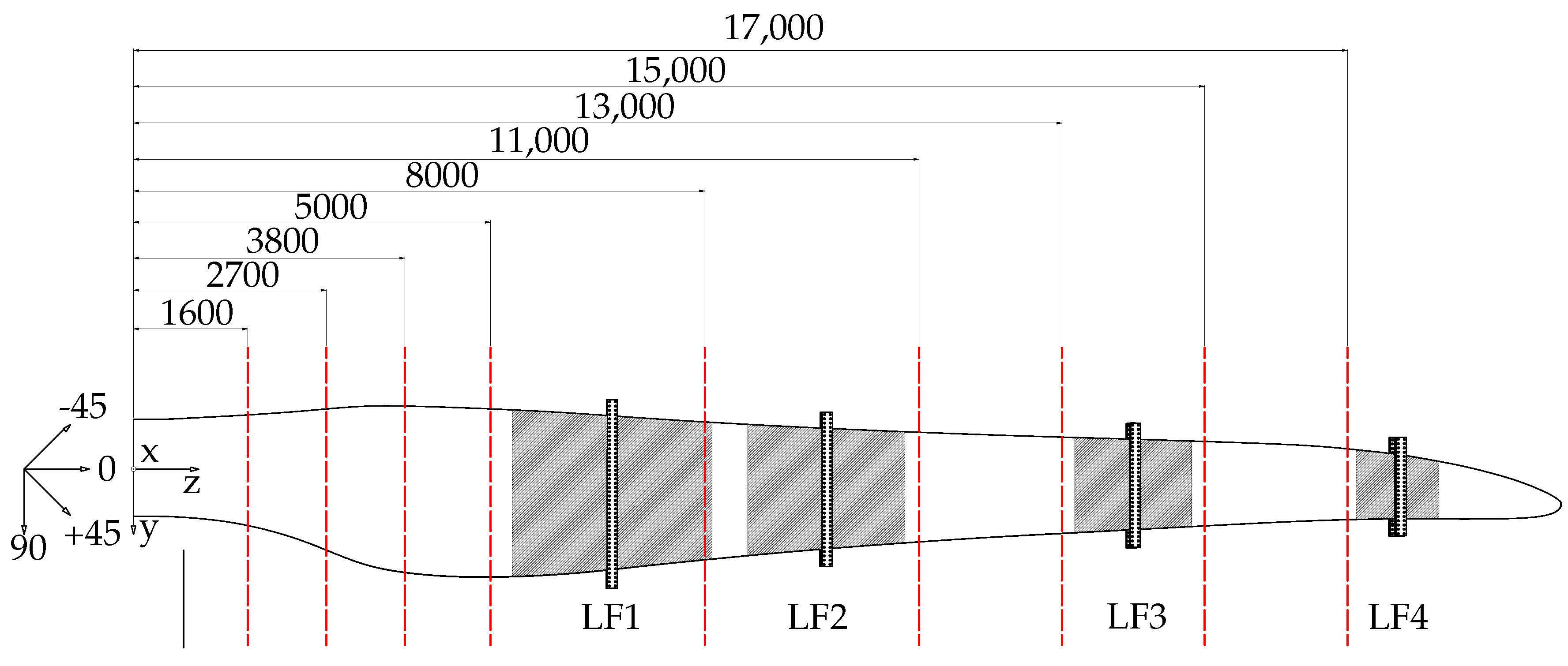
The static tests were performed for the first produced 20 $\mathrm{m}$ rotor blade. All the tests were conducted in the 90 $\mathrm{m}$ test hall of Fraunhofer IWES in Bremerhaven, Germany from 23 January to 6 February 2018, and the test description and the raw data are given in [8]. Figure 1 shows the experimental setup. The description of the test is based on the technical report of Bernd Haller from Fraunhofer IWES [8]. The rotor blade coordinate system is defined in Figure 2 and corresponds to the IEC 61400-5:2020 [9] B-system. The origin was placed in the centre of the cylindrical part of the blade root on the flange. The z-axis pointed to the rotor blade tip along the cylinder axis, the y-axis pointed to the trailing edge at 0° pitch angle and the x-axis was obtained from $e_x=e_y\times e_z$ in the illustrated configuration.

As shown in Figure 1a, the rotor blade was attached to a metal frame at the root (left side of the figure). This metal frame, now called the root jig, had an angle of 7.5° of the flange plate to the vertical orientation (Figure 3b). The blade z-axis was inclined by this angle to the ground. In numerical pre-studies, this angle was included, but no substantial effect on the numerical results (displacements and mechanical strains) was observed. For the static tests, the external loads were introduced by utilising load frames; see Figure 1b and Appendix A for size and geometry. As shown in Figure 1a, the load frames were connected by wires to hydraulic cylinders which applied the loads. Load cell sensors were used to measure the applied load at load frame, and draw wire displacement sensors (DWS) were used to measure the vertical displacements at the load frames and at the tip. Two DWS measurement positions for each load frame existed. They are defined as leading and trailing edge positions for all load cases. For the two Mx load cases, the leading edge position refers to the left-hand side position of the load frame, and the trailing edge position refers to the right-hand side. The views are given in Figure 4a,b. For all experiments two DWS were used. For the flapwise bending, one was placed on the leading edge and one at the trailing edge. For the edgewise bending, the DWS were placed on the suction side and at the pressure side. In addition to the DWS, an optical displacement sensor was used to measure the three dimensional deformation of the rotor blade. The twisting of the rotor blade root and the rotation of the load frames were measured using angle measurement sensors.

The root jig is shown in Figure 3. The analysis of the stiffness has shown that it is softer in x direction. The static tests are not affected by it, but the modal analysis of the clamped rotor blade is [10].

The local structural deformation of the rotor blade was measured with strain gauges at various locations along the span, as shown in Figure 2. For the span positions $L=$ 5000 $\mathrm{m}$$\mathrm{m}$ and $L=$ 8000 $\mathrm{m}$$\mathrm{m}$, the blade sections are strongly instrumented to be able to obtain the deformation of the cross-sections itself.

The relative measurement error of the strain gauges was $\pm 2\%$. The absolute error was determined analysing the zero load time signals. It was ≈±0.5–2 $\mathsf{\mu }$$\mathrm{m}$/$\mathrm{m}$. To guarantee the quality of the measurements, climate sensors were used to measure the temperature and humidity inside the test hall at regular intervals.

The rotor blade was subjected to flapwise and edgewise bending tests, and furthermore, to three torsion tests. The four bending tests were named:

• Mxmax: leading edge under compression;
• Mxmin: trailing edge under compression;
• Mymax: suction side under compression;
• Mymin: pressure side under compression.

The three torsion test were named:

• LC1: Torsional stiffness test at load frame 2.
• LC2: Torsional stiffness test at load frame 3.
• LC3: Torsional stiffness test at load frame 4.

2.1.1. Bending Stiffness Tests

For the load case Mxmax (leading edge under compression) the rotor blade was oriented in the 0° pitch position with the trailing edge facing upwards, cf. Figure 4a. The rotor blade was loaded at load frames 1 and 4; cf. Figure 2. For the load case Mxmin (trailing edge under compression), the rotor blade was rotated by an angle of 180° compared to the Mxmax orientation. In this case the leading edge was facing upwards; cf. Figure 4b. For this load case, the rotor blade was loaded at the load frames 2, 3 and 4. For the load case Mymax (suction side under compression), the rotor blade was rotated by an angle of 90° compared to the Mxmax orientation with the pressure side facing upwards; cf. Figure 4c. For this load case, the rotor blade was loaded at the load frames 2, 3 and 4.

For the load case Mymin (pressure side under compression), the rotor blade was rotated to an angle of 270° compared to the Mxmax orientation with the suction side facing upwards; cf. Figure 4d. The rotor blade was loaded on the outer three load frames for both these load cases. For this load case, the rotor blade was loaded at the load frames 2, 3 and 4.

Quasi static loading was achieved by slowly increasing the loads in four load steps (i.e., 40%, 60%, 80% and 100%). The 100% loads for all the load cases used for validation are shown in

Table 1. Applied loads measured by load cells for all the bending load cases.

Load Point	Length [mm]	Mxmax [kN]	Mxmin [kN]	Mymax [kN]	Mymin [kN]
1	6700	10.1	0.0	0.0	0.0
2	9700	0.0	6.5	21.8	14.9
3	14,000	0.0	11.3	18.8	19.8
4	17,700	12.6	6.3	24	15.9

.

2.1.2. Torsional Stiffness Tests

The rotor blade was oriented with the pressure side upwards for all three load scenarios (cf. Figure 4b). Only one load frame was loaded with a pair of parallel forces pulling vertically up and down, respectively. The upper attachment was mounted in the shear centre and the lower attachment at the end of the frame near the trailing edge.

• For test LC1, due to a mistake, the upper attachment was shifted 158 $\mathrm{m}$$\mathrm{m}$ toward the leading edge.
• For test LC1, the load frame 1 was dismounted; for test LC2, the load frames 1 and 2 were dismounted; and for test LC3, the load frames 1, 2 and 3 were dismounted to reduce stiffening effects.

The loading and the measurement points for the three load cases LC1–LC3 at load frames 2, 3 and 4 are shown in Figure A1a–c, respectively. The test scenarios with the applied loads are shown in

Table 2. Loads applied by load cells and load frame positions for all the torsion load cases.

Scenario	Length [mm]	Load up [kN]	Load down [kN]
LC1	9700	18.7	30.0
LC2	14,000	29.1	30
LC3	17,700	31.6	30.0

.

To determine the twist angle, the draw wire displacement sensors and angle sensors were used. The distances between the draw wire displacement sensors are given in

Table 3. DWS for all the torsion test scenarios.

Length [mm]	Distance ${\mathit{d}}_{\mathbf{DWS}}$ [mm]
	Load Case 1	Load Case 2	Load Case 3
6700	2923	2923	2923
9700	3178	2500	2500
14,000	2717	2717	2050
17,700	2375	2375	2375

. By assuming that the deformations of the load frames themselves are negligible, these distances and the separate displacements can be used to find the twist angles $\alpha$:

$$\alpha ={sin}^{-1}\left(\frac{u_{DW{S}_2}-u_{DW{S}_1}}{d_{DWS}}\right).$$

(1)

2.2. Experimental Setup for Modal Tests

The setup for the modal test is given in [11]. The measurements were performed in the clamped configuration described in Section 2.1 and in a free–free configuration. The free–free configuration was realised using long rubber belts with a low eigenfrequency, which did not influence the eigenfrequencies of the rotor blade.

3. Model

The reference model was based on the given design of the 20 $\mathrm{m}$ Smartblades 2 rotor blade. The model’s creation started with the aerodynamic hull. The spar, spar caps and adhesive bonds were modelled in the finite element framework Abaqus. All sections, the model segments and material definitions were created in Abaqus. The final finite element mesh was then translated to the input data format for the finite element tools Ansys and Nastran. In the following sections the model is explained in detail.

3.1. Material and Layup

The materials and their properties are given in

Table 4. Material parameters based on [12]. 1—Values after matrix infusion.

Material	Orientation	E${}_1$ [MPa]	E${}_2$ [MPa]	G${}_{12}$ [MPa]	${\mathit{\nu }}_{12}$ [-]	$\mathit{\rho }$ [kg/m${}^3$]	h [mm]
UD	0${}^{°}$	44,151	14,526	3699	0.3	1948	0.827
2AX45	$\pm {45}^{°}$	11,316	11,316	11,978	0.633	1875	0.625
2AX90	$0^{°}$/90${}^{°}$	26,430	27,520	3464	0.124	1875	0.651
3AX	$0^{°}$/±45${}^{°}$	29,873	13,377	6918	0.466	1875	0.922
3AX manual layup	$0^{°}$/±45${}^{°}$	21,888	9473	5126	0.46	1658	1.318
Balsa Baltek SB.100		35	35	105	0.3	291 ${}^1$	19.05
Foam Airex C70-55-20mm-spar		55	55	22	0.3	180 ${}^1$	20
Foam Airex C70-55-20mm		55	55	22	0.3	279 ${}^1$	20
Foam Airex C70-55-15mm		55	55	22	0.3	314 ${}^1$	15
Foam Airex C70-55-10mm		55	55	22	0.3	384 ${}^1$	10
Foam Airex C70-55-5mm		55	55	22	0.3	596 ${}^1$	5
ADH/HARDENER		4864	4864	1828	0.33	1160	-
Pseudo material		10	10	3.84	0.3	1.0 × 10${}^{-5}$	0.1

[12]. Three material classes are used to build the wind turbine blade. Glass fibre reinforced plastics (GFRP), foam material for sandwich stiffened regions and an adhesive material to glue the parts of the rotor blade. The foam material consider the effect of matrix infusion which leads to larger density. As an additional material, the pseudo-material was added. It can be used to select specific regions within the finite element model. The names or the material numbers of Abaqus, Ansys and Nastran are given in

Table 5. Material numbers in the finite element models.

Material	Abaqus	Ansys	Nastran
UD	MAT_UD	7	7
2AX45	MAT_2AX-45_45	22	22
2AX90	MAT_2AX-0_90	24	24
3AX	MAT_3AX	18	18
3AX manual layup	MAT_3AX_HANDLAMINAT	4	4
Balsa Baltek SB.100	MAT_BALSA_SB100	12	12
Foam Airex C70-55-20mm-spar	MAT_SCHAUMSTEGAIREX_C70-55	32	32
Foam Airex C70-55-20mm	SCHAUM_AIREX_C70-55-20MM	37	37
Foam Airex C70-55-15mm	SCHAUM_AIREX_C70-55-15MM	25	25
Foam Airex C70-55-10mm	SCHAUM_AIREX_C70-55-10MM	19	19
Foam Airex C70-55-5mm	SCHAUM_AIREX_C70-55-5MM	13	13
ADH/HARDENER	ADH/HARDENER	23	23

.

3.2. Finite Element Model

3.2.1. General Remarks

The rotor blade model (cf. Figure 5) was created within the finite element software Abaqus by meshing the aerodynamic surface and the shear web plane. The thin walled structures were modelled with quadratic serendipity finite shell elements (STRI65, S8R). For the thick adhesive joints, quadratic serendipity finite solid elements (C3D20R) were used. For Ansys and Nastran the corresponding elements were used. For all models, modal analysis simulations were performed. As expected, they had the same results, and all models can be used equally for validation purposes. In further analysis, due to the expensive license of Abaqus, this program was only used for the modal analysis. The static and the mass distribution analyses were done using Ansys.

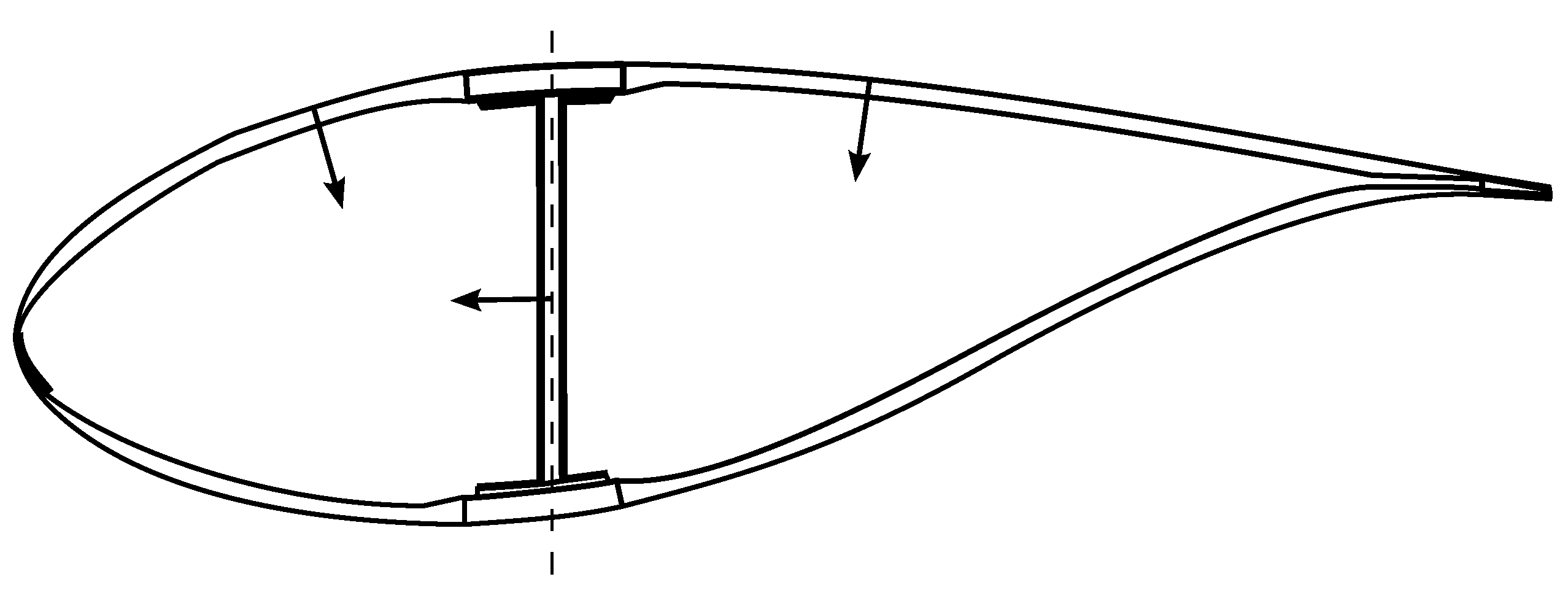
The layups are defined as stacking sequences. The material formulation within the elements utilises the classical lamination theory [13] with all its assumptions. The stacking directions for the suction side shell, pressure side shell and the spar caps are given in Figure 6. As a consequence, the middle plane of the shell had an offset to shell element nodes. Homogenised material properties for the individual layers were used, meaning fibres and matrix were not separate materials. A transversal isotropic material symmetry was assumed for the single glass fibre layers. The balsa woods, used as a sandwich core, were part of the stacking sequence and had isotropic material symmetry. The biaxial and triaxial layups were defined as one thick layer with homogenised parameters. All material properties can be found in detail in Table 4. The material numbers or names used in the different finite element models are given in Table 5. For better usability, several pseudo-layers/materials were defined to allow the selection of sets and components; i.e., multiple pseudo-materials existed for some components, e.g., root and suction side. The pseudo-material numbers and corresponding components are given in

Table A3. List of materials given in Table 4.

Name	Explanation	Abaqus	Ansys	Nastran
Pseudo Material	all elements between 0–1 m	MATPOS_0-1000MM	1	1
Pseudo Material	all elements between 6–7 m	MATPOS_6000-7000MM	2	3
Pseudo Material	all elements between 12–13 m	MATPOS_12000-13000MM	3	3
3AX manual layup	triaxial glass fiber manual layup	MAT_3AX_HANDLAMINAT	4	4
Pseudo Material	all elements between 15–16 m	MATPOS_15000-16000MM	5	5
Pseudo Material	all trailing edge elements	MATPOS_TE	6	6
UD	unidirectional glass fiber	MAT_UD	7	7
Pseudo Material	all elements between 18–19 m	MATPOS_18000-19000MM	8	8
Pseudo Material	all elements of the spar cap	MATPOS_SPARCAP	9	9
Pseudo Material	all elements between 14–15 m	MATPOS_14000-15000MM	10	10
Pseudo Material	all elements between 4–5 m	MATPOS_4000-5000MM	11	11
Balsa Baltek SB.100	Balsa wood material	MAT_BALSA_SB100	12	12
Foam Airex C70-55-5mm	Foam material	SCHAUM_AIREX_C70-55-5MM	13	13
Pseudo Material	all elements of the suction side	MATPOS_SS	14	14
Pseudo Material	all elements between 3–4 m	MATPOS_3000-4000MM	15	15
Pseudo Material	all elements between 11–12 m	MATPOS_11000-12000MM	16	16
Pseudo Material	all elements of the root	MATPOS_ROOT	17	17
3AX	all elements between 12–13 m	MAT_3AX	18	18
Foam Airex C70-55-10mm	Foam material	SCHAUM_AIREX_C70-55-10MM	19	19
Pseudo Material	all elements between 16–17 m	MATPOS_16000-17000MM	20	20
Pseudo Material	all elements between 2–3 m	MATPOS_2000-3000MM	21	21
3AX manual layup	all elements between 12–13 m	MAT_2AX-45_45	22	22
3AX manual layup	all elements between 12–13 m	ADH/HARDENER	23	23
3AX manual layup	all elements between 12–13 m	MAT_2AX-0_90	24	24
Foam Airex C70-55-15mm	Foam material	SCHAUM_AIREX_C70-55-15MM	25	25
Pseudo Material	all elements between 1–2 m	MATPOS_1000-2000MM	26	26
Pseudo Material	all elements between 9–10 m	MATPOS_9000-10000MM	27	27
Pseudo Material	all elements between 13–14 m	MATPOS_13000-14000MM	28	28
Foam Airex C70-55	Foam material (not used)	MAT_SCHAUMSTEGAIREX_C70-55	29	29
Balsa Baltek SB.150	Balsa wood material (not used)	SB150	30	30
Pseudo Material	all elements for the end of the spar to tip	MATPOS_REST	31	31
Foam Airex C70-55-20mm-spar	Foam material in the spar	SCHAUM_AIREX_C70-55-20MM_STEG	32	32
Pseudo Material	all elements between 17–18 m	MATPOS_17000-18000MM	33	33
Pseudo Material	all elements of the belts	MATPOS_BELT	34	34
Pseudo Material	all elements between 10–11 m	MATPOS_10000-11000MM	35	35
Pseudo Material	all elements of the pressure side	MATPOS_PS	36	36
Foam Airex C70-55-20mm	Foam material	SCHAUM_AIREX_C70-55-20MM	37	37

.

3.2.2. Differences from the Design

To reduce the complexity of the model, several assumptions and adaptations were used within the finite element model. In this section, these differences from the design are illustrated.

In contrast to Figure 6, the core material was not chamfered in the trailing edge area (Figure 7), where the direct bond of suction and pressure sides was present. In consequence, this led to a higher local bending stiffness at the trailing edge. E.g., the analysis of trailing edged buckling load as described by [14] will be overestimated. Additionally, local strain measurements at the trailing edge will be affected and may result in larger deviations. On a global scale or sufficiently far from the trailing edge, the effects can be expected to be small, because the additional tensile stiffness due to the core material is very small.

In the finite element model, all adhesive joints were thicker compared to the designed rotor blade. The adhesive was modelled with three-dimensional volume elements between the reference planes of the shell elements. The reference planes were the aerodynamic shape of the rotor blade; cf. Figure 6.

As a result, the thickness of all adhesive joints was increased by the thickness of the local design layup. This is illustrated in Figure 8a. The thin blue line is the reference plane. If the thickness shell elements are included (cf. Figure 8b) an overlap occurs. The thicker adhesives will change the mass distribution of the rotor blade and have an impact on its stiffness. Both effects are assumed to be small.

Further, the adhesive joint at the leading edge has not been modelled. It is very thin and was assumed to be negligible.

Due to the finite shell element formulation, there was overlap between the shell elements and volume elements, and between shell elements at the trailing edge illustrated in a cross-section in Figure 8b.

For manufacturing reasons the root was built separately. In a later process the root was joined to the rest of the rotor blade. This skew adhesive joint has not been modelled. Further, neither bolts for the rotor blade connection nor the T-bolt connection were included in the FE model in detail.

Another simplification was made at the tip of the rotor blade. The lighting protection aluminium tip was not modelled. The tip does not effect static measurements and due to the small weight (Section 4.2) could only have a minor impact on the modal results. Due to its shape, the meshing of the region is challenging, and it adds more elements without adding additional information.

3.2.3. Boundary Conditions

The root jig consisted of very thick steel frames. It was shown that the stiffness of the frame was very high in z direction perpendicular to the ground. Parallel to the ground it was softer. This is relevant for the eigenfrequency tests but not for the static tests. A clamped boundary condition has been assumed. For all root nodes all translations and rotations were set to zero (fixed in all six DOF).

3.2.4. Load Introduction

The loads in the experiment were introduced with load frames for the different load cases, which are listed in Table 1. The load frames were simplified for the finite element model. They were realised as pilot nodes connected with infinite stiff connections to the outer shell of the rotor blade model. The mass distribution of the frame was not considered and did not influence the experimental results. The deformation sensors and strain gauges were set to zero in the state, where all weights were already applied.

The rotor blade was connected to the root jig in an angle of 7.5° in relation to the ground. This angle influences the load introduction, because the load vector is perpendicular to the ground. This means for the torsion load cases that torsional moment is not parallel to the rotor blade z-axis (i.e., the pitch axis). However, the angle between the load vector and the rotor blade z-axis was smaller than 7.5° due to the weight of the rotor blade and the load frames. The simulation of one bending and one torsion case show that the error in displacements is lower than 0.1% if the angle is not taken into account. Therefore, the load vector has not been adapted for all other load cases.

4. Analysis

4.1. Validation with Static Tests

4.1.1. Scenarios and Variations

All experimental scenarios are given in Table 1 for the bending load cases and in Table 2 for torsion load cases. All these experiments were modelled in Ansys Mechanical.

4.1.2. Solver

All static finite element analyses were performed with a linear static solver which does not take large deformations, large rotations or the effect of profile deformation due to the rotor blade bending into account.

4.1.3. Bending—Displacements

For all four bending load scenarios the displacements at four specific positions at the leading and trailing edge were measured. The positions were $L=$ 6700, 9700, 14,000 and 17,700 mm. The measurements were done at the load frame. To compare the results, the measured displacements were mapped to the surface using a linear function. For the two Mx load cases the leading edge position refers to the left-hand side position of the load frame and the trailing edge position refers to the right-hand side. The views are given in Figure 4a,b. A comparison between the simulation and the experiment at each position for the four bending load cases is shown in Figure 9a–d. All numerical results are in good agreement with the corresponding experimental data. The biggest difference was found in load case Mymax. A significantly more pronounced bending–torsion coupling was measured for this load case compared to simulation. This behaviour cannot really be explained, because the Mymin load case did not show such behaviour. The blade was rotated by 180° in both load cases (Mymin and Mymax) and the amplitudes were in the same order of magnitude, but the magnitude of the bending–torsion coupling was different. The simulation did not show this behaviour.

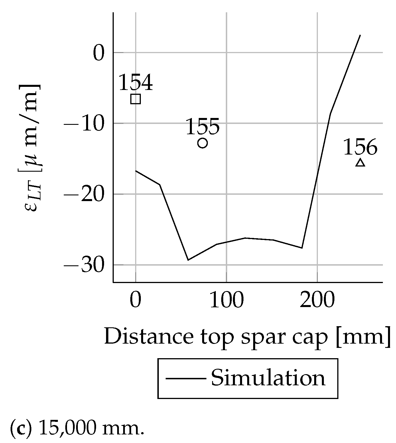
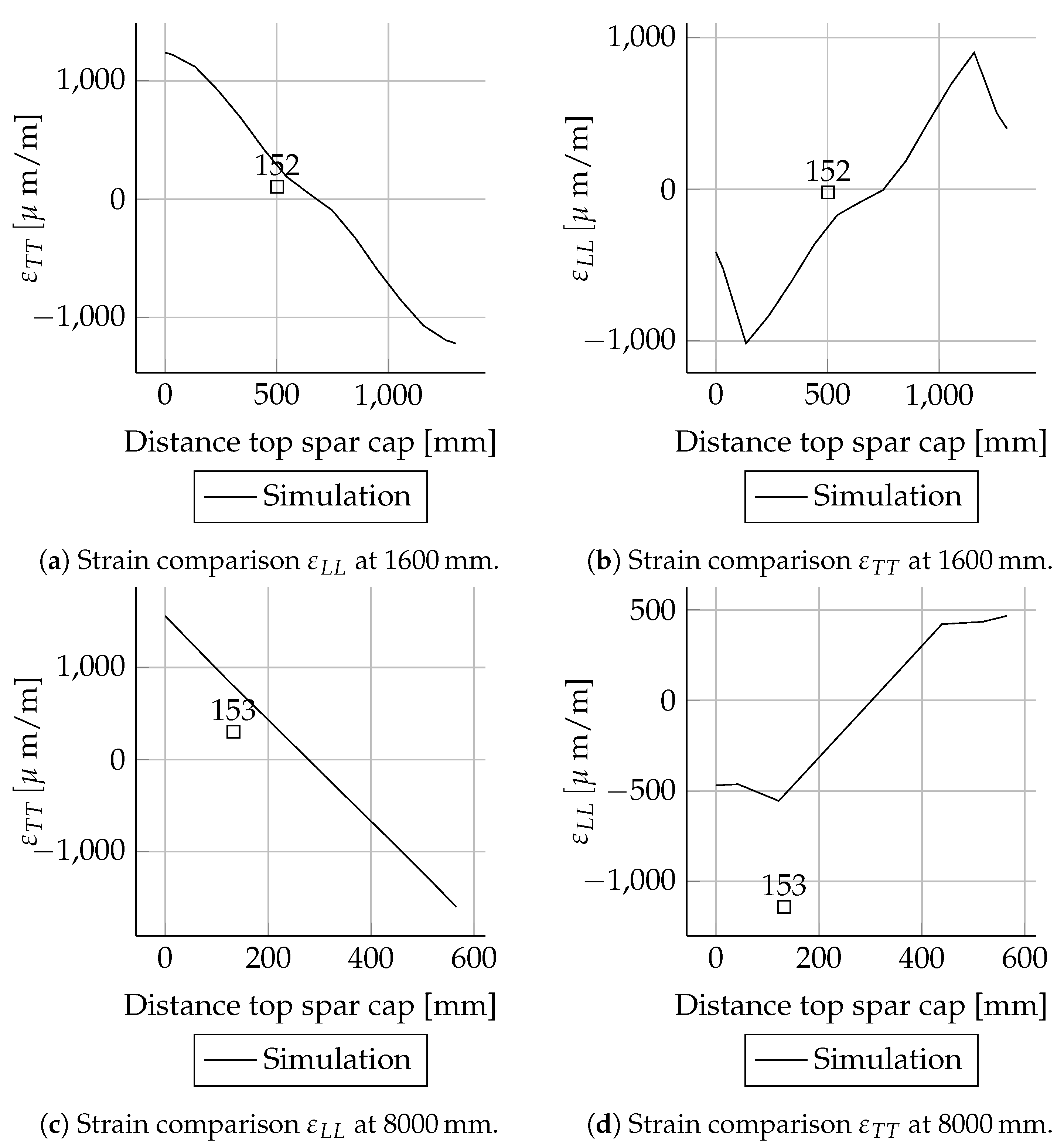
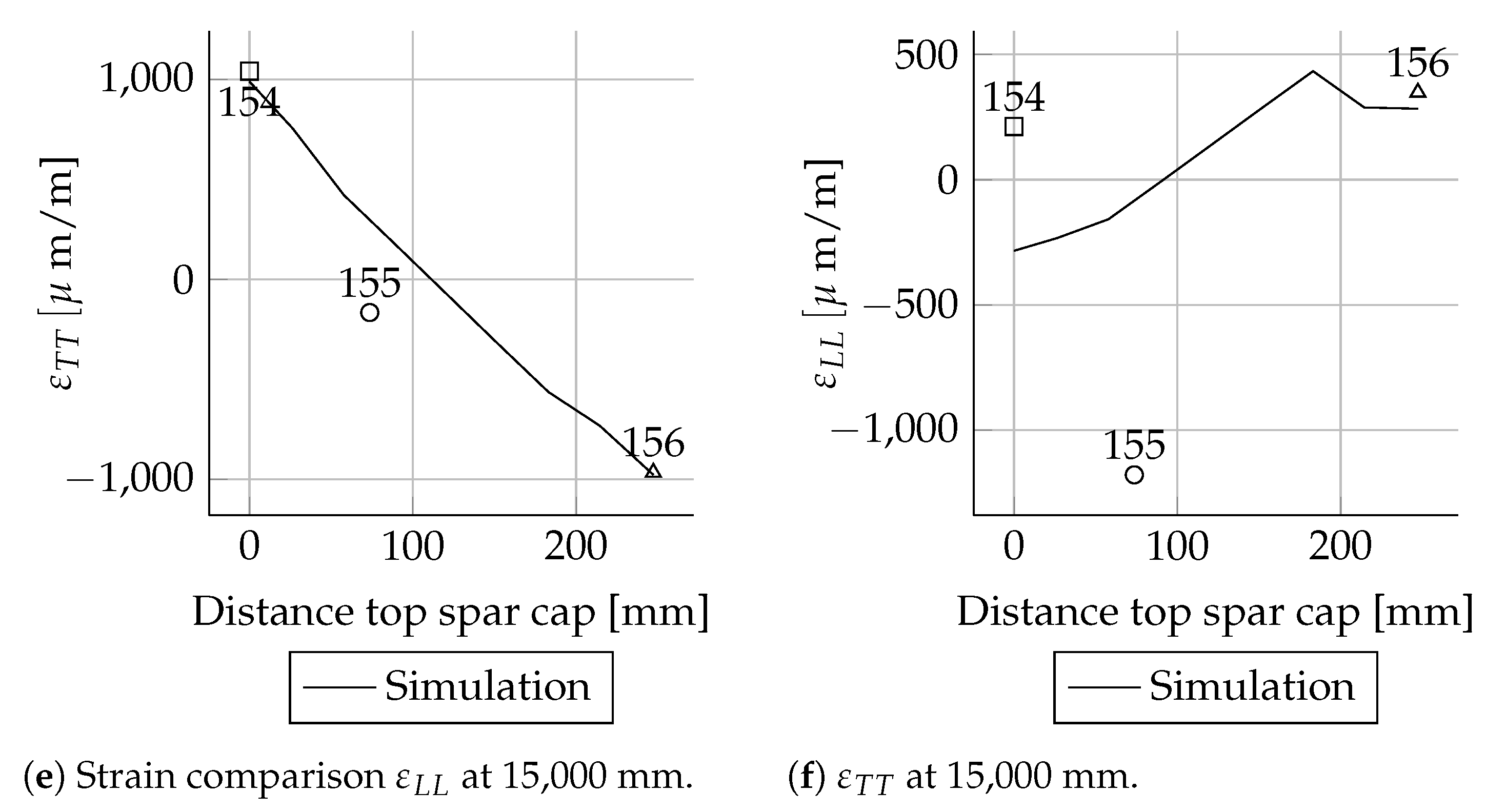
For three positions (1600, 8000 and 15,000 mm) the spar caps were instrumented with additional strain gauge rosettes. The components of a strain gauge rosette ${\epsilon }_a$, ${\epsilon }_b$ and ${\epsilon }_c$ illustrated in Figure 10 had to be transformed to the strain components in local laminate coordinates (L—longitudinal in $0^{°}$ direction; T—transversal in ${90}^{°}$ direction) ${\epsilon }_{LL}$, ${\epsilon }_{TT}$ and ${\epsilon }_{LT}$ [15].

For $\alpha ={45}^{°}$, $\beta ={45}^{°}$ and the engineering shear strain defined as ${\gamma }_{LT}={\epsilon }_{LT}+{\epsilon }_{TL}=2{\epsilon }_{LT}$ we get

$$\begin{array}{cc}\hfill {\epsilon }_{LL}& ={\epsilon }_a\hfill \\ \hfill {\epsilon }_{TT}& ={\epsilon }_c\hfill \\ \hfill {\epsilon }_{LT}& ={\epsilon }_b-\frac{{\epsilon }_a+{\epsilon }_c}{2}\hfill \end{array}$$

(2)

The sensors used for ${\epsilon }_a$, ${\epsilon }_b$ and ${\epsilon }_c$ are given in

Table A2. List of sensor combinations to extract the shear strain based on Equation (2).

Position [mm]	Number	${\mathit{\epsilon }}_{\mathit{a}}$	${\mathit{\epsilon }}_{\mathit{b}}$	${\mathit{\epsilon }}_{\mathit{c}}$
1600	152	008_Z01600_SW_TE_+45	007_Z01600_SW_TE_00	009_Z01600_SW_TE_-45
8000	153	115_Z08000_SW_TE_+45	114_Z08000_SW_TE_00	116_Z08000_SW_TE_-45
15,000	154	141_Z15000_SS_SC_+45	140_Z15000_SS_SC_00	142_Z15000_SS_SC_-45
15,000	155	144_Z15000_SW_TE_+45	143_Z15000_SW_TE_00	145_Z15000_SW_TE_-45
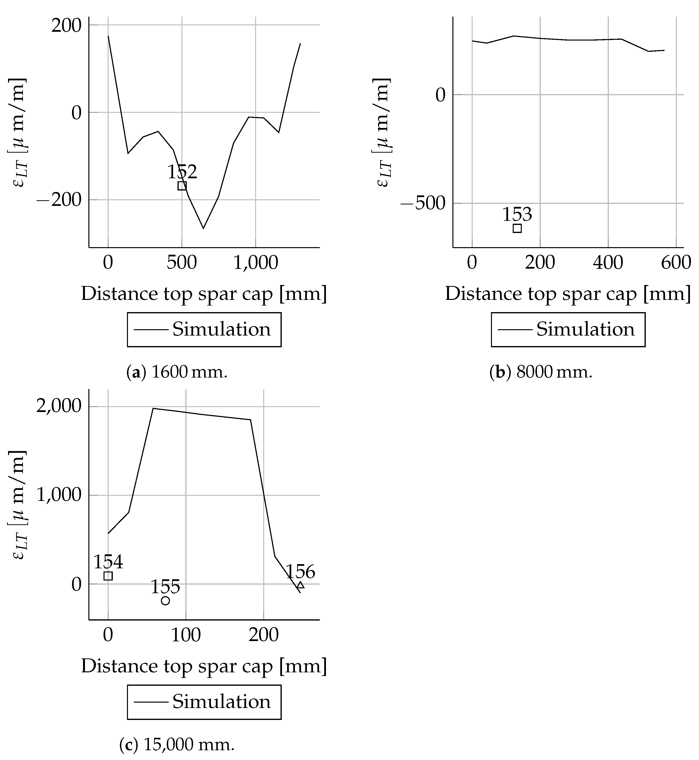
15,000	156	135_Z15000_PS_SC_+45	134_Z15000_PS_SC_00	136_Z15000_PS_SC_-45

. These measurements are not considered for validation because of poor instrumentation.

Mxmax Results

The results for the load case Mxmax (cf. Figure 4a) are shown in Appendix D.1. Due to the orientation of the rotor blade and the loading in edgewise direction, it can be expected that the mechanical strains at leading and trailing edge are higher compared to the spar cap strains. Both the simulation and the experiment fulfilled that expectation; cf. Figure A2 for the mechanical strains at the spar caps and Figure A3, Figure A4, Figure A5, Figure A6, Figure A7, Figure A8, Figure A9, Figure A10, Figure A11 and Figure A12 for the mechanical strains of the leading and trailing edges.

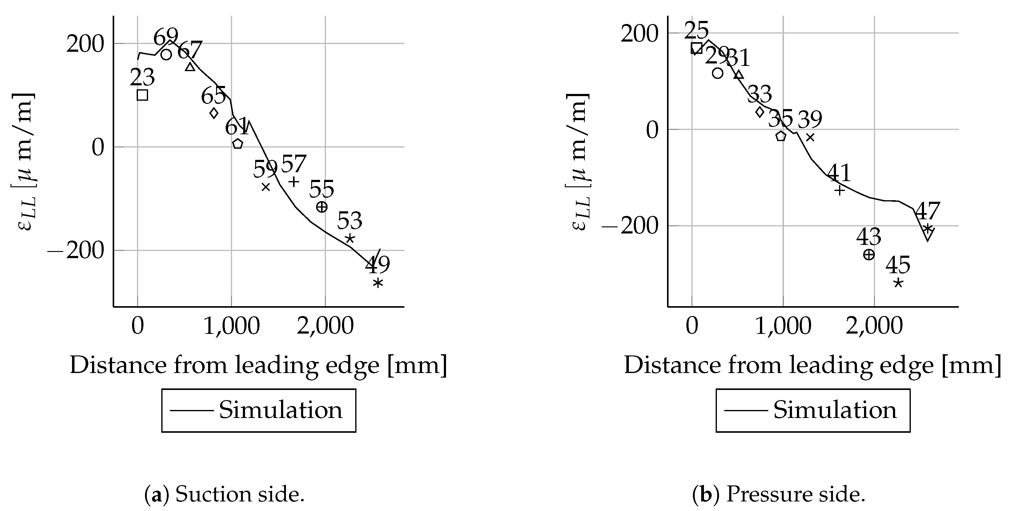
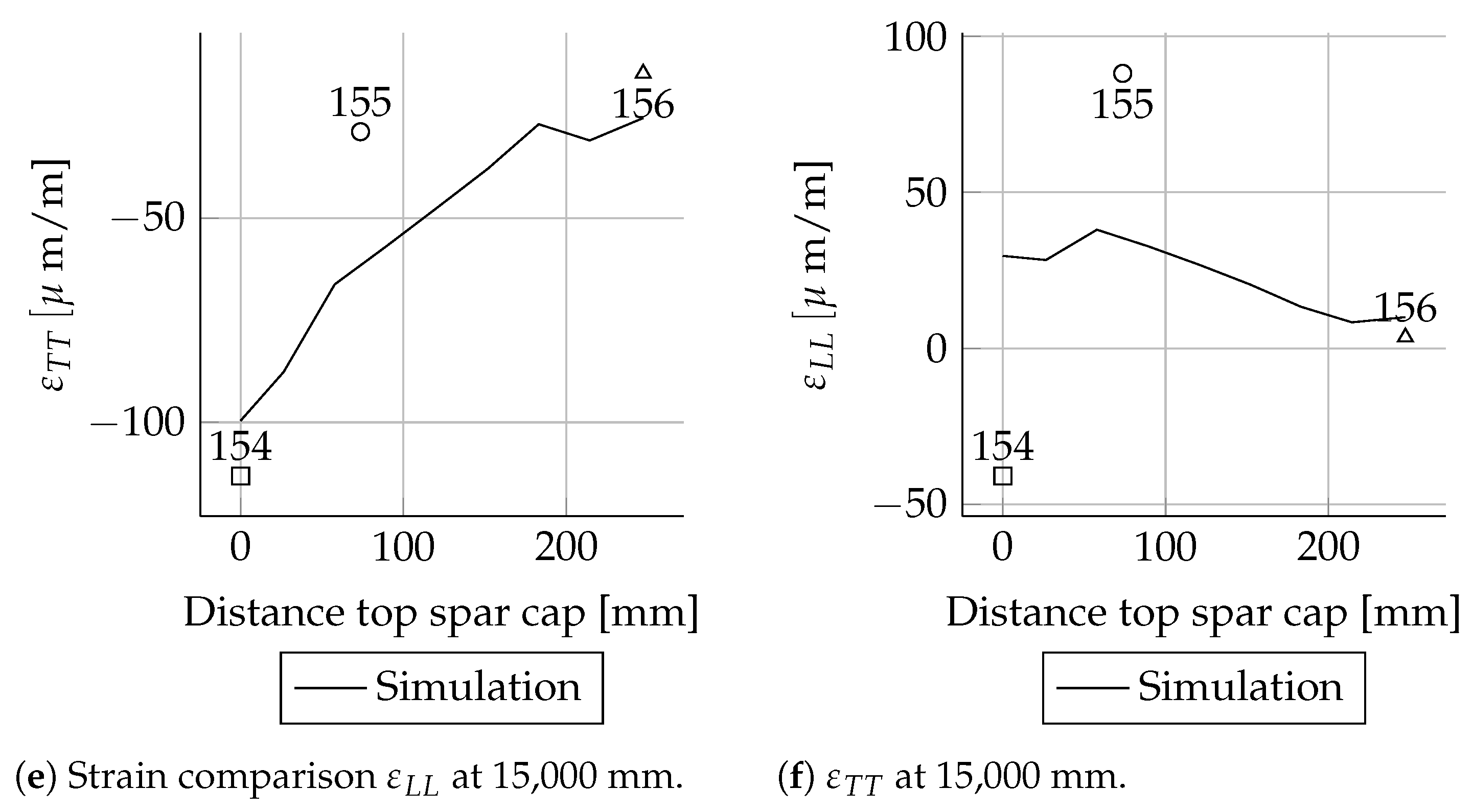
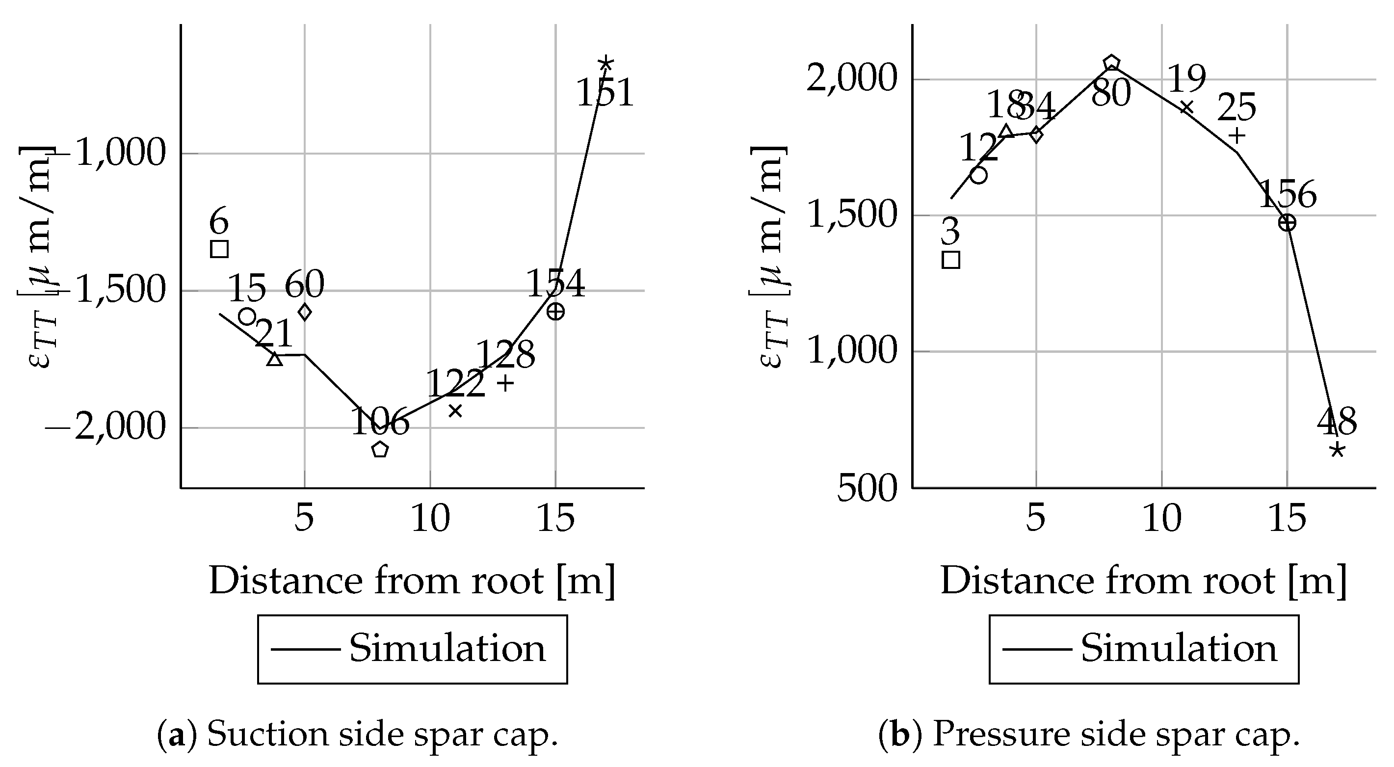
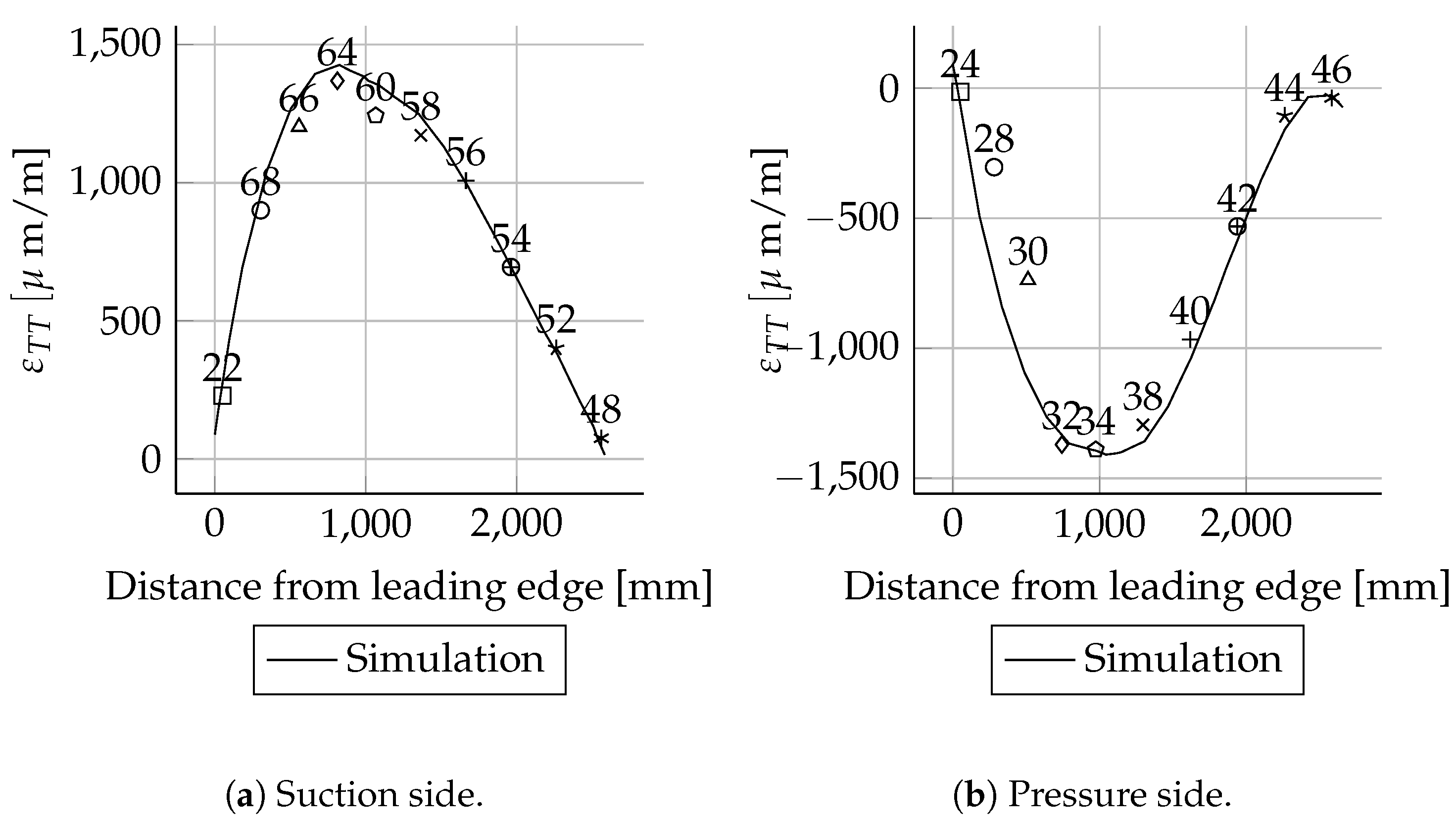
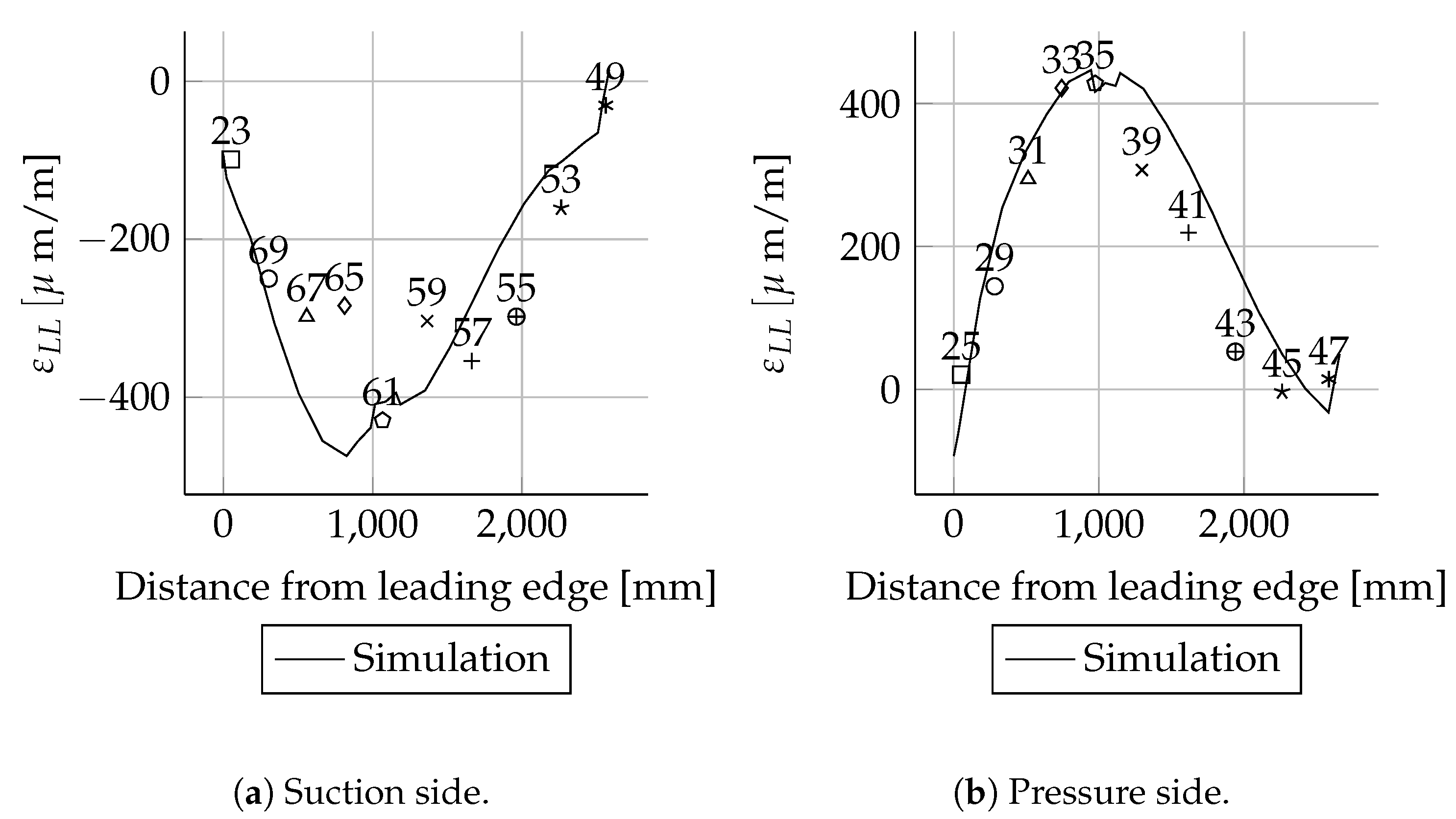
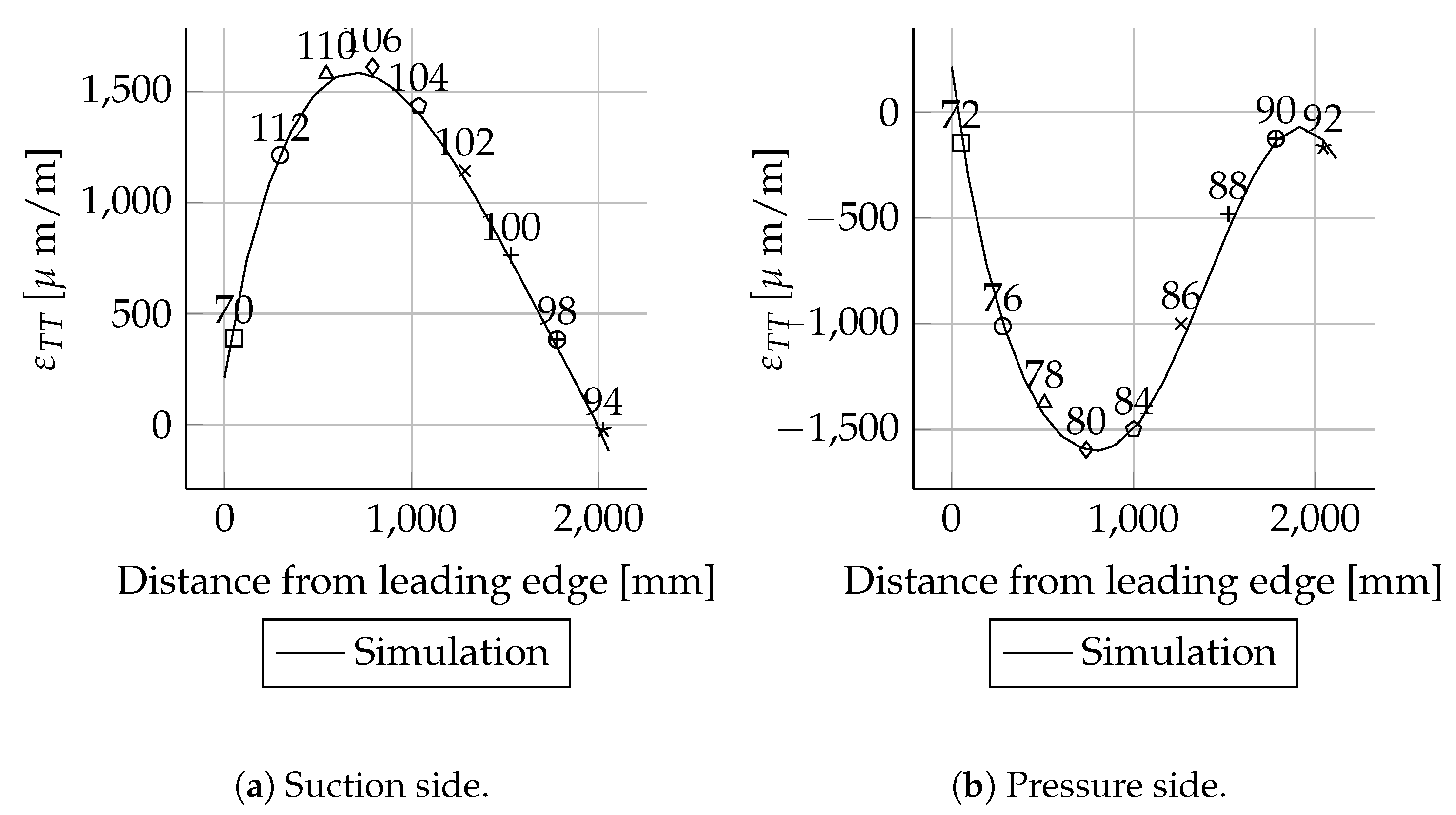
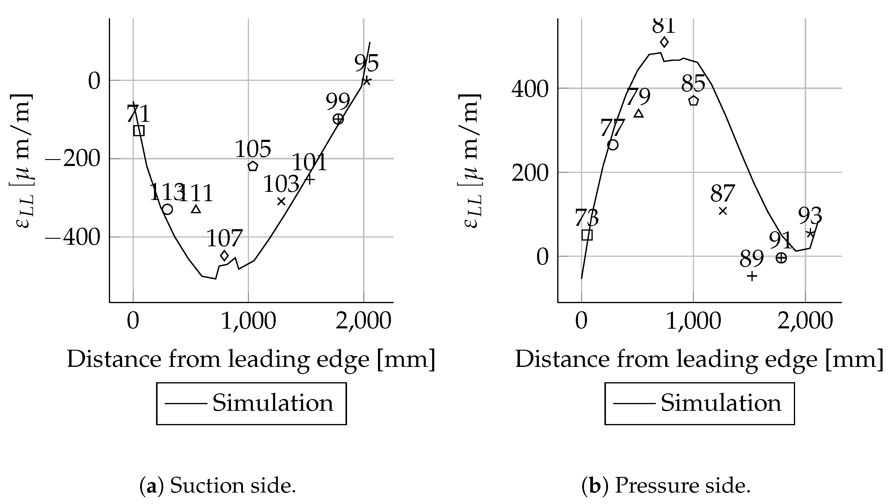
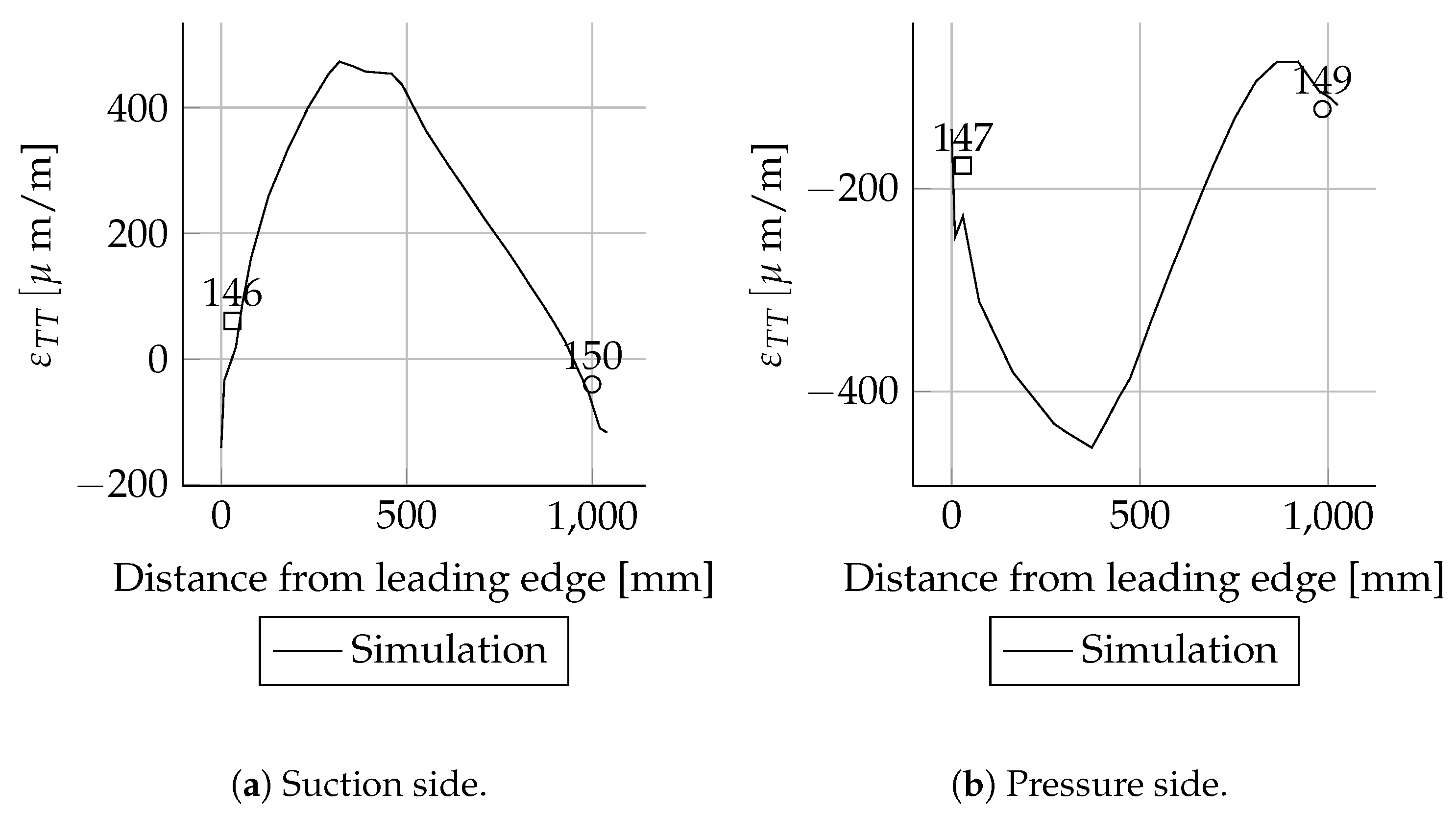
The absolute deviations were small for most positions. As expected, the relative deviations were higher in areas with small mechanical strains than in areas with larger mechanical strains. This behaviour can be seen very well when comparing the mechanical strains of the suction side spar cap with the pressure side spar cap. The deviations of the strains were less than 20 $\mathsf{\mu }$$\mathrm{m}$$\mathrm{m}$. These are in the range of absolute error values for strain gauges. Therefore, the deviations are relatively high. The mechanical strains of the suction side match well between simulations and experiments. In the case of the pressure side, there are bigger differences close to the root.

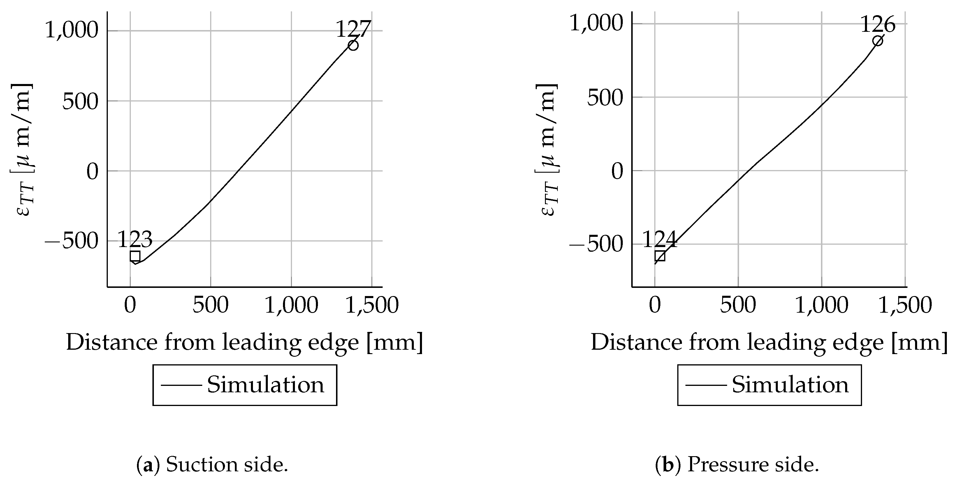
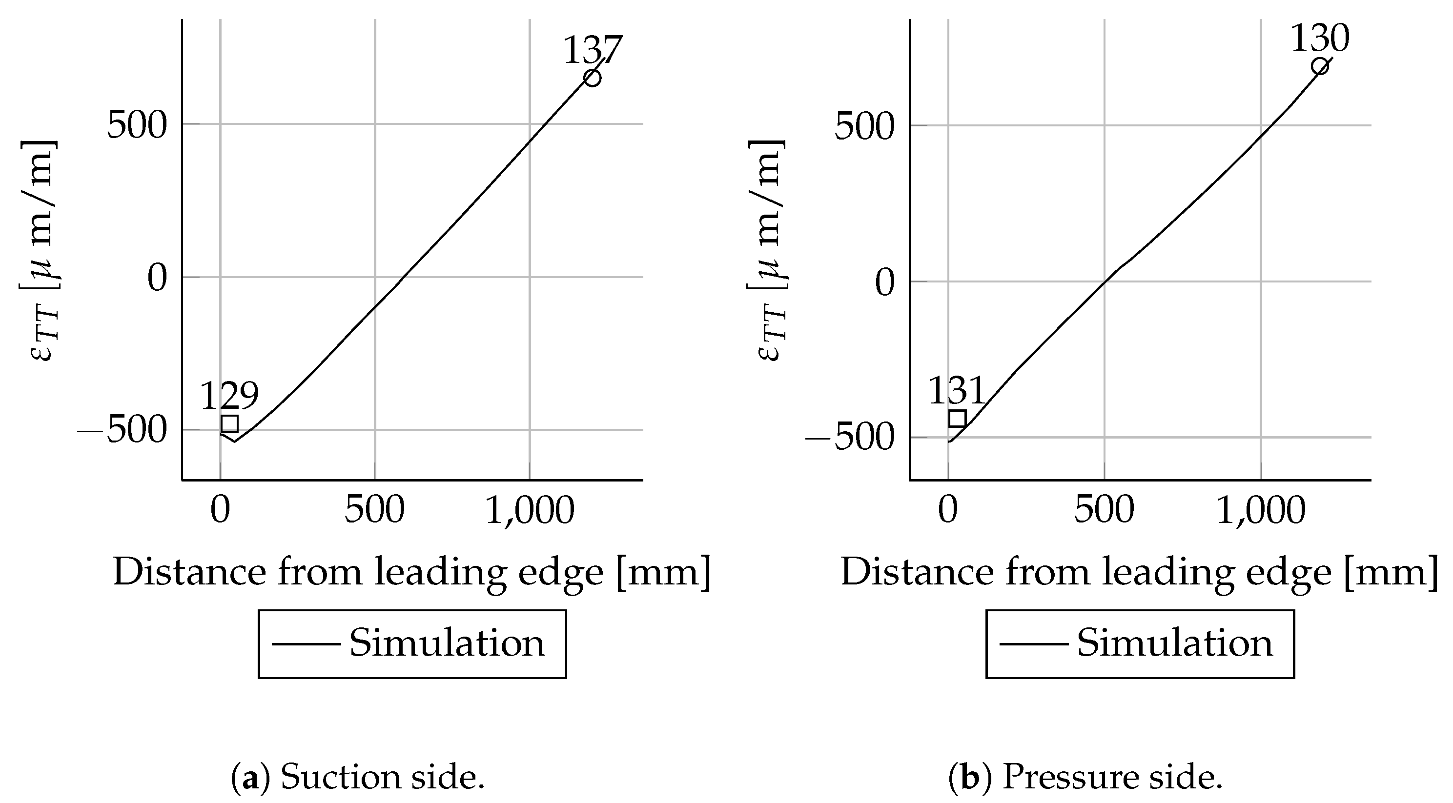
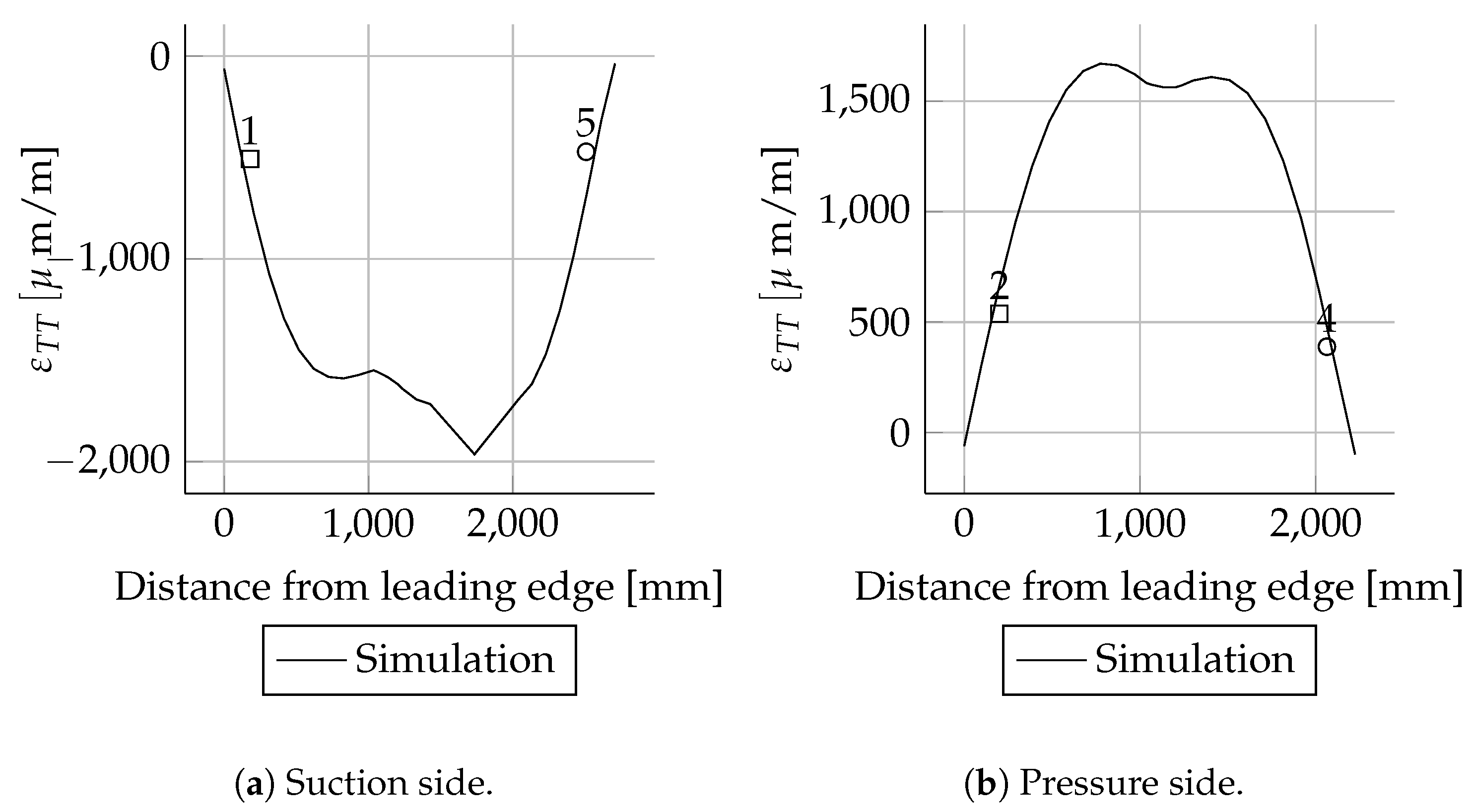
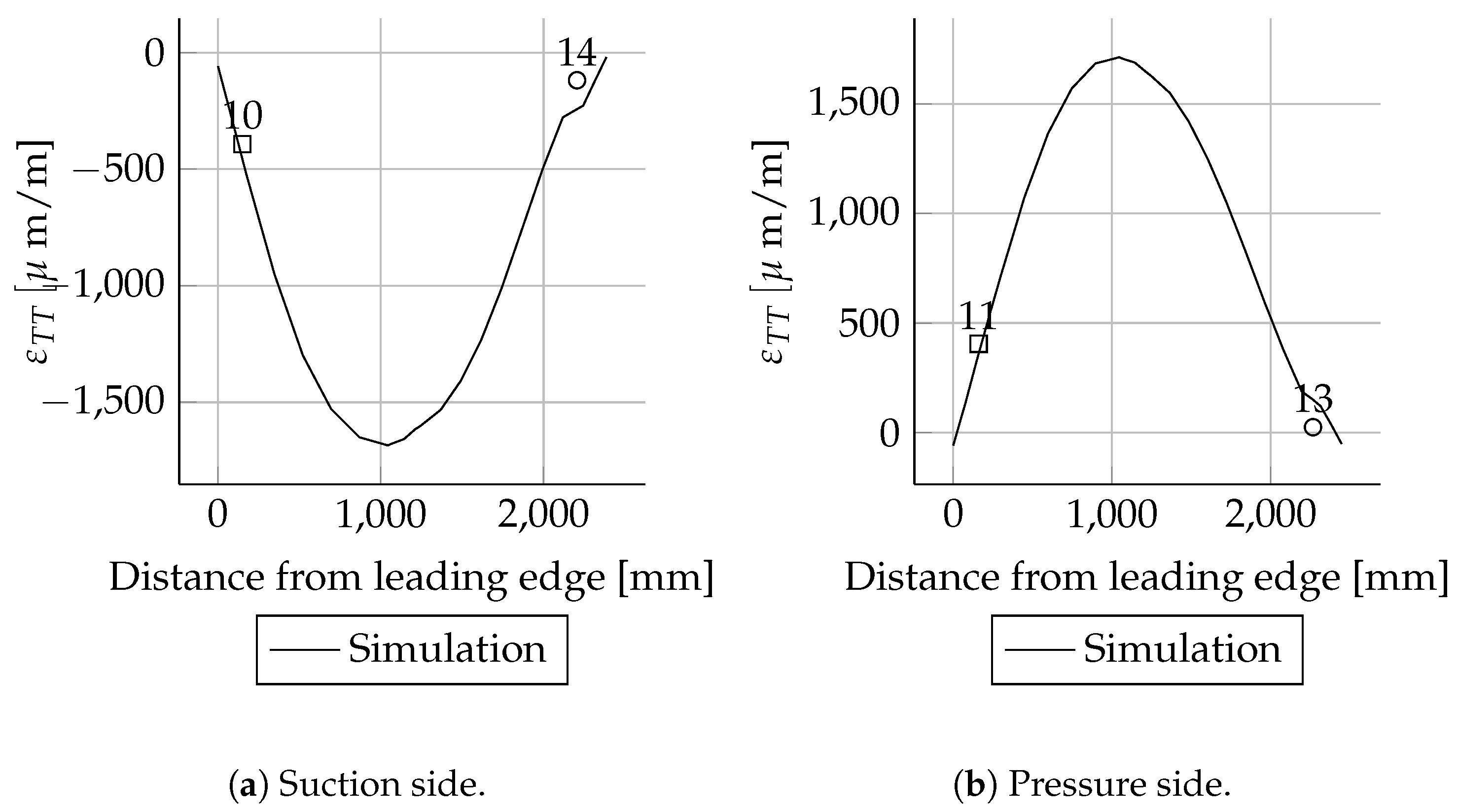
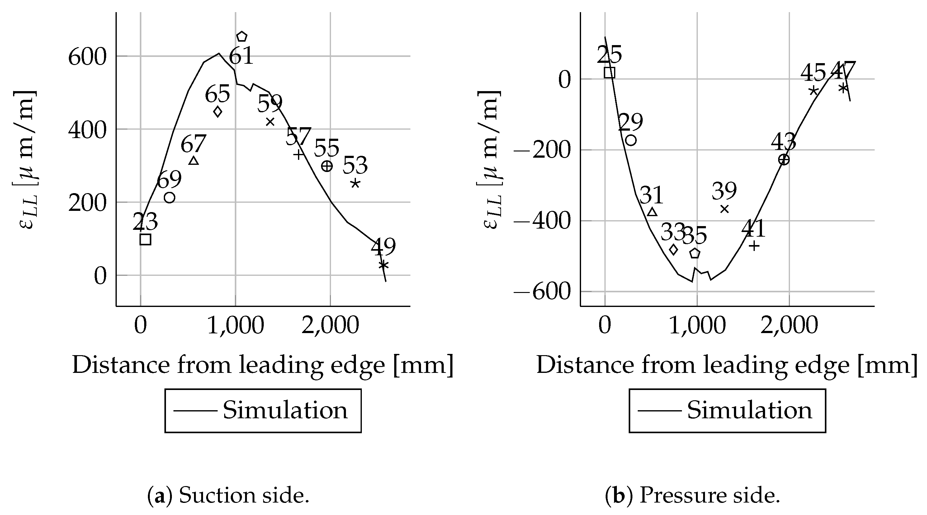
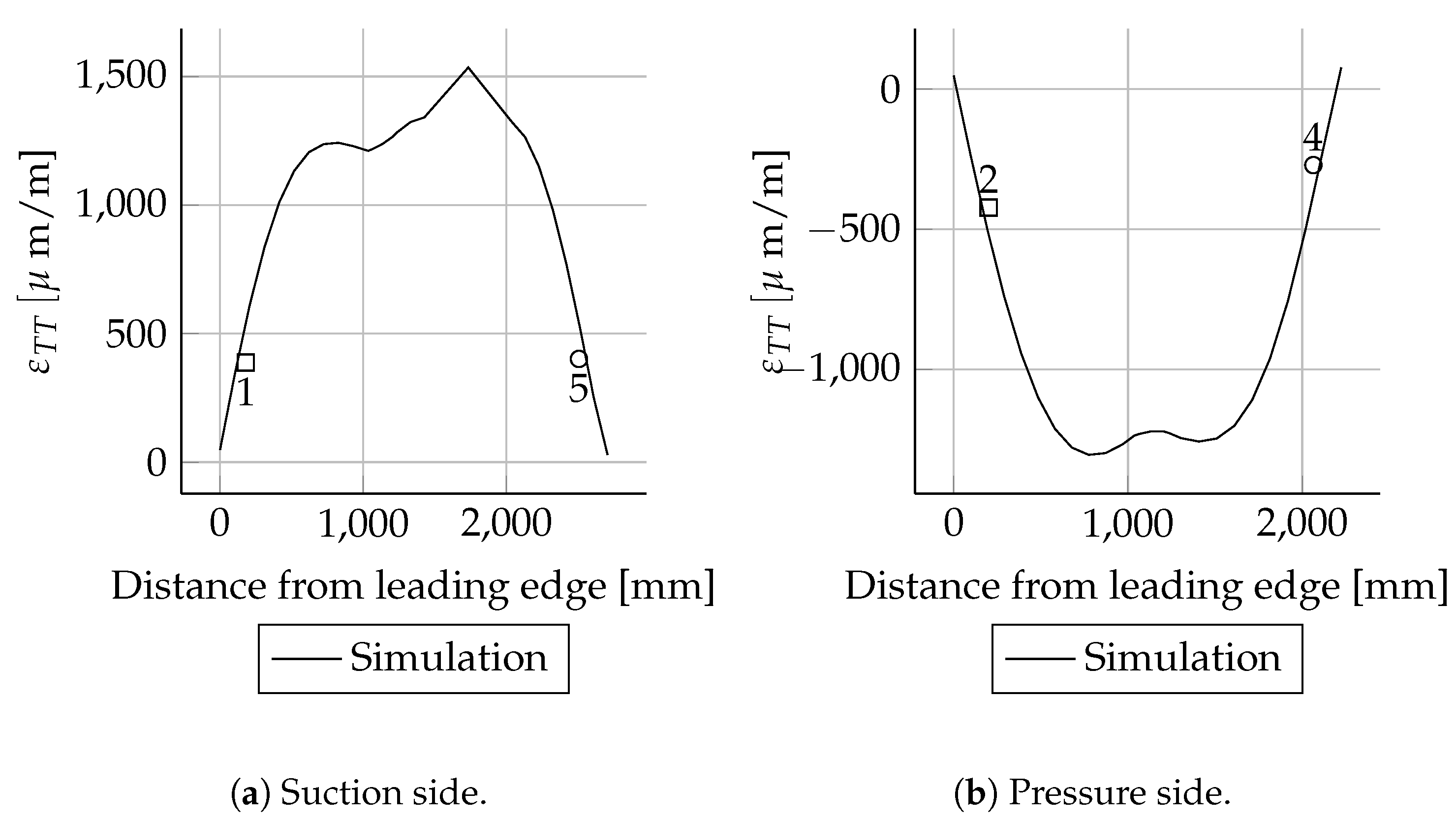
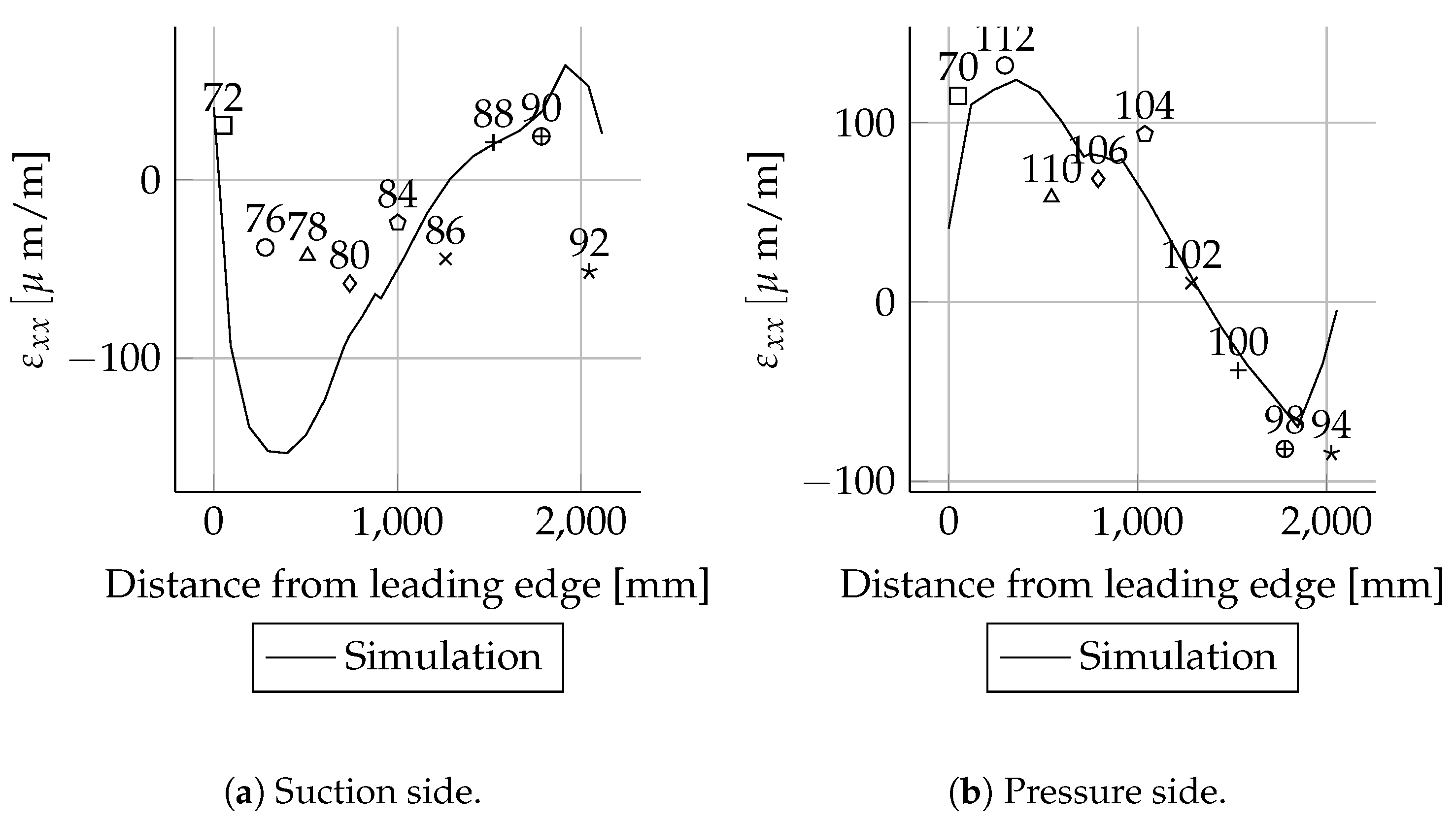
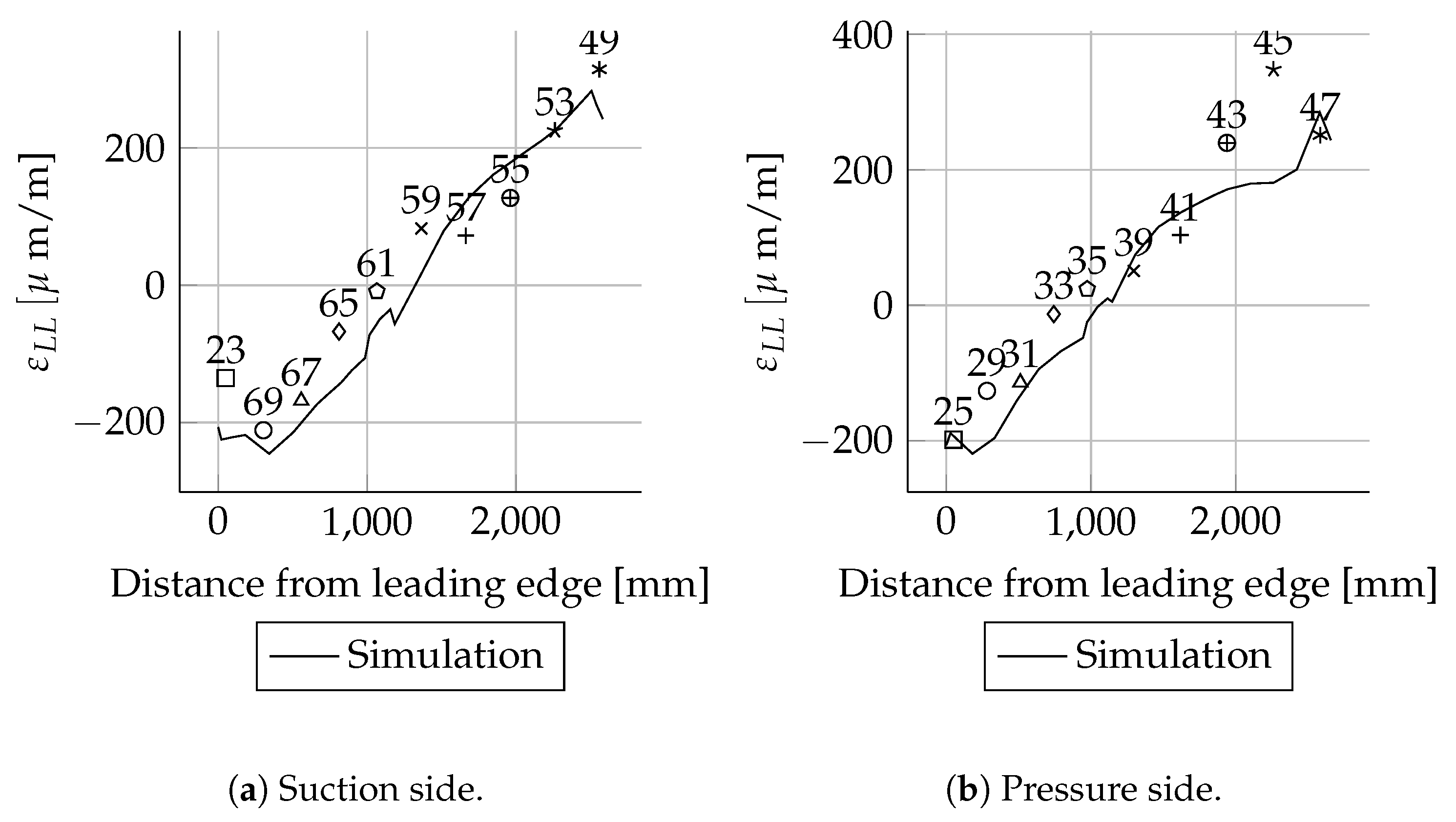
The comparison of the mechanical strains between the experimental and numerical results of the heavily instrumented cross-sections at $L=$ 5000 and $L=$ 8000 $\mathrm{m}$$\mathrm{m}$ are shown in Figure A5, Figure A6, Figure A7 and Figure A8. Both the simulated ${\epsilon }_{LL}$ (cf. Figure A5a) and ${\epsilon }_{TT}$ (cf. Figure A6a) strain distributions at the suction side are in very good agreement with the experimental results at $L=$ 5000 $\mathrm{m}$$\mathrm{m}$. 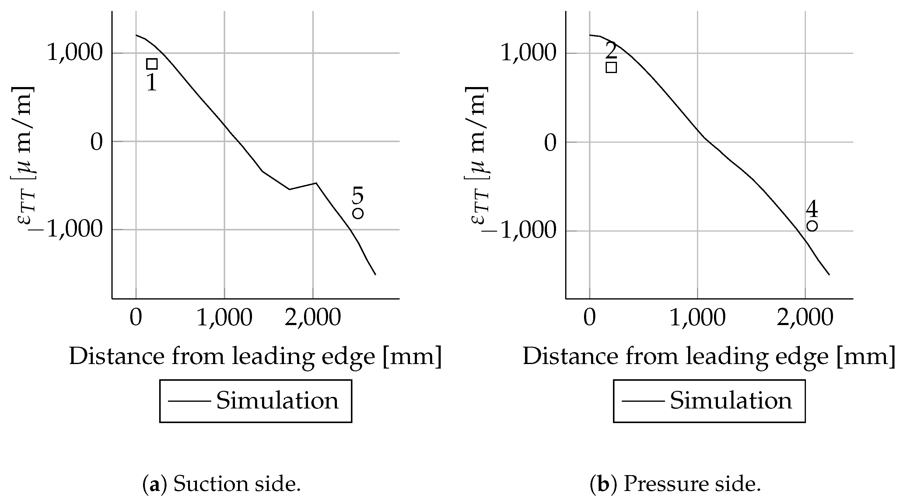For the results of ${\epsilon }_{LL}$ at the pressure side (cf. Figure A5b), the mechanical strain distribution between 0 and 800 $\mathrm{m}$$\mathrm{m}$ from the leading edge differs between the experiments and the simulations. It is not clear where this non-linearity came from, because the suction side did not show such behaviour. For ${\epsilon }_{TT}$ at the pressure side, this distribution error did not occur. However, the strain between 1800 and 2200 $\mathrm{m}$$\mathrm{m}$ was underestimated by the simulation (cf. Figure A6b).

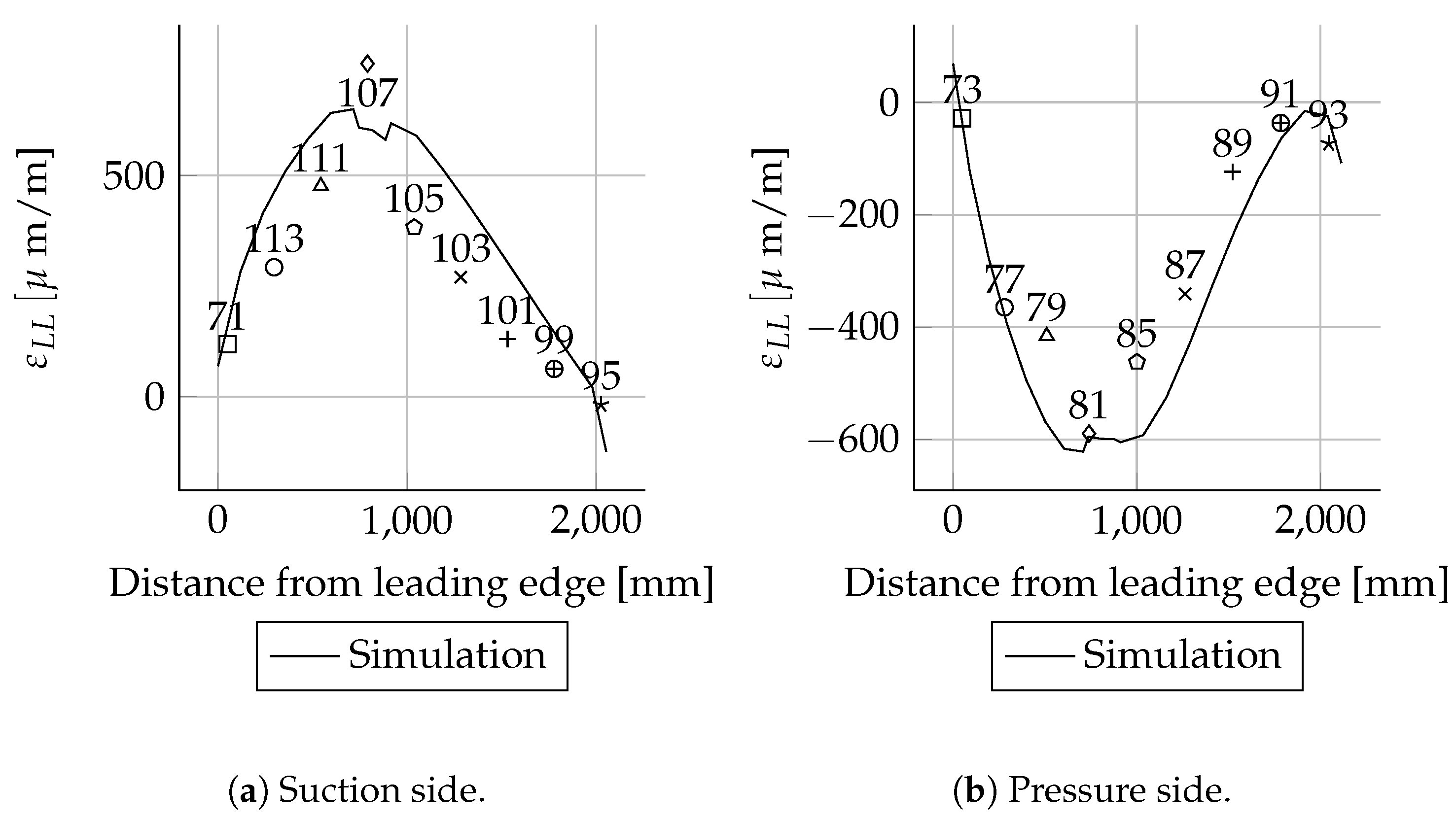
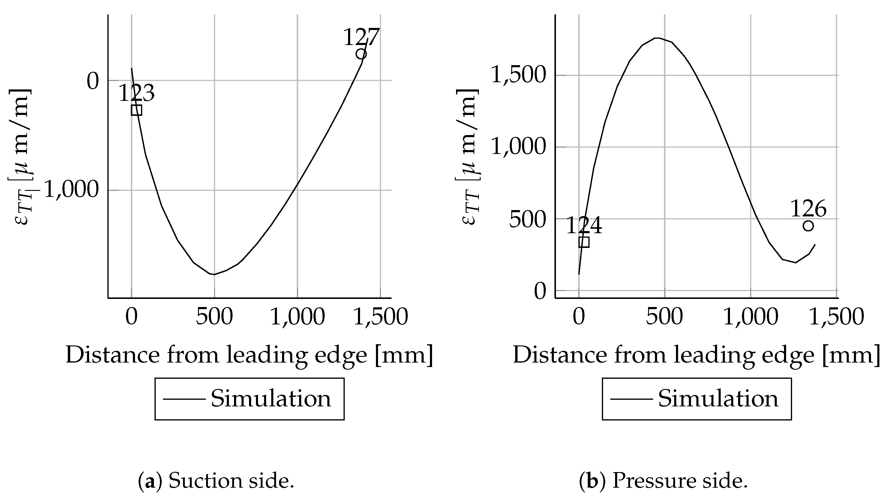
For $L=8000 \mathrm{m}\mathrm{m}$ the simulated ${\epsilon }_{TT}$ suction side (cf. Figure A7a) and pressure side (cf. Figure A7b) strain distribution values are in very good agreement with the experiment. The simulated ${\epsilon }_{TT}$ strains for the suction side match also with experiments (cf. Figure A8). For the pressure side the experiment shows a weak non-linear strain distribution, and the strain distribution of the numerical results is nearly linear (cf. Figure A8b).

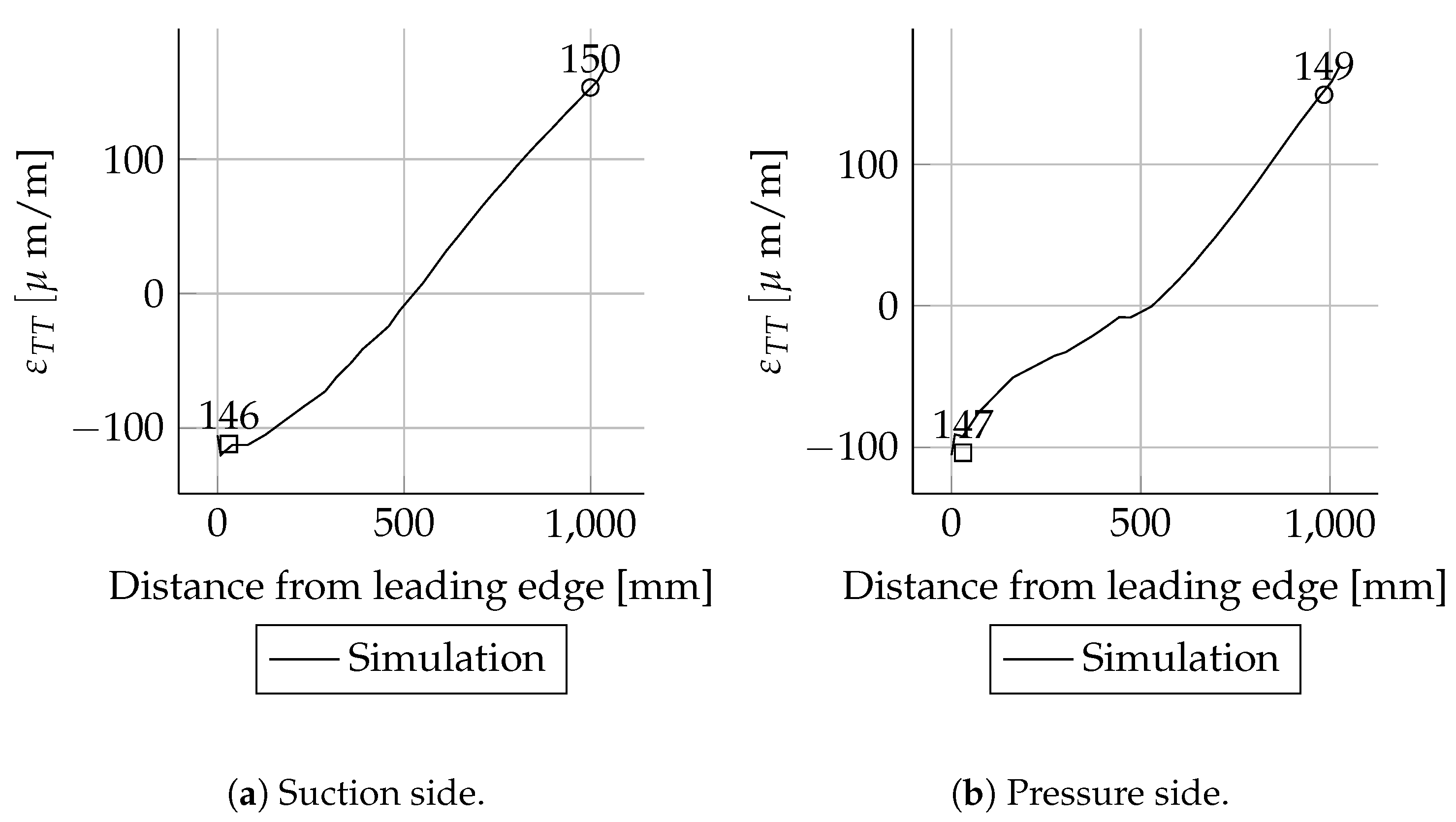
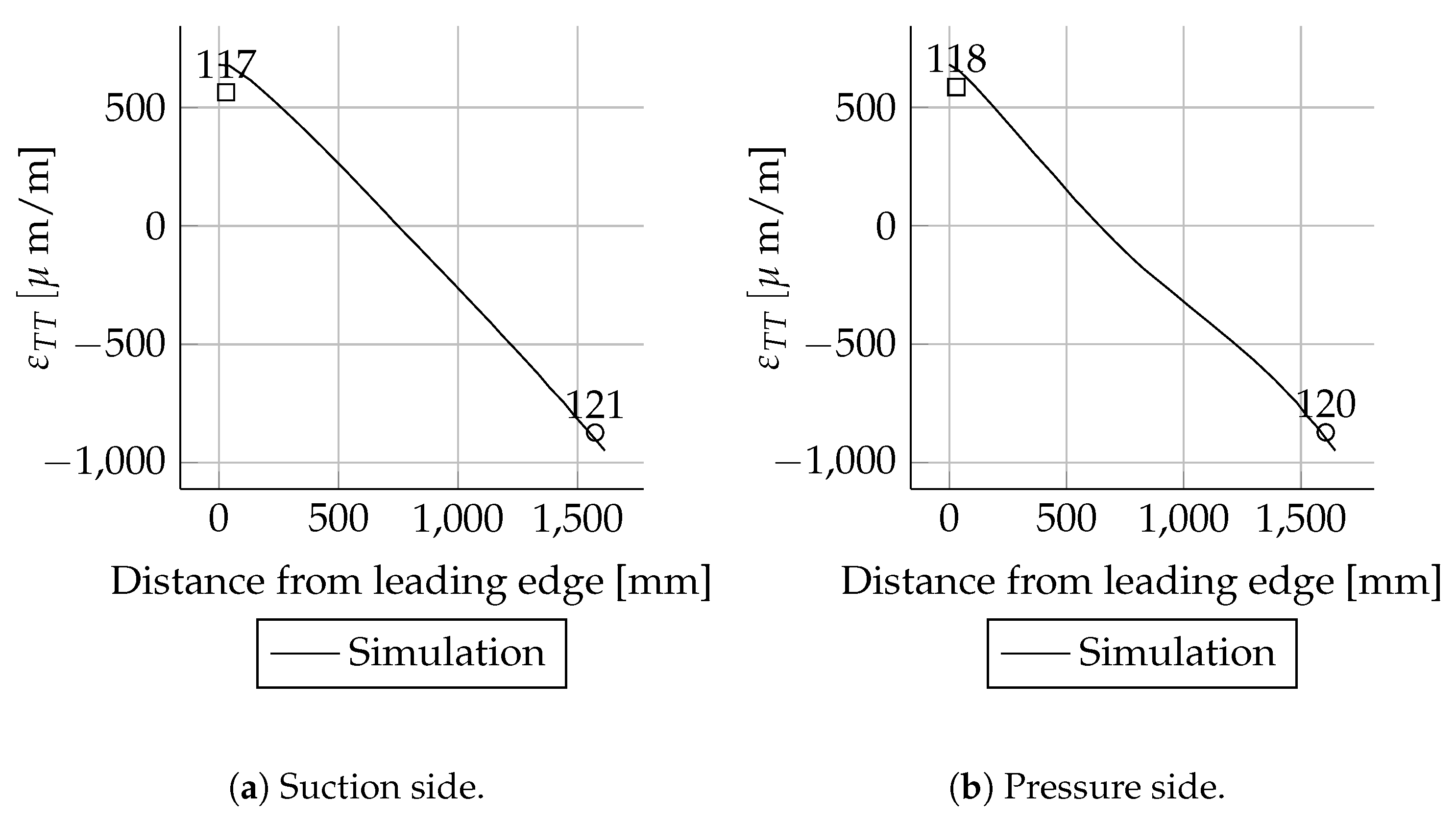
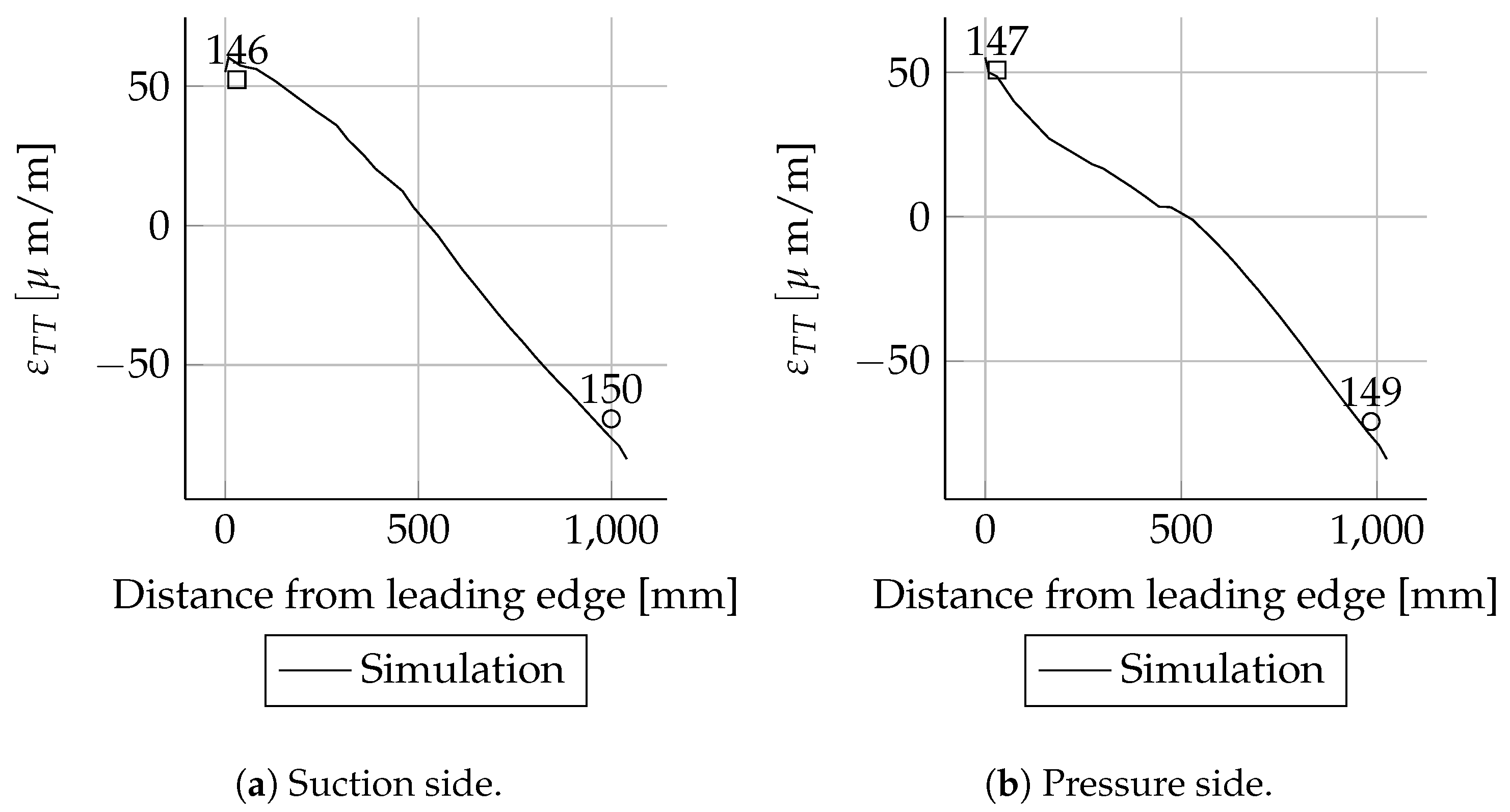
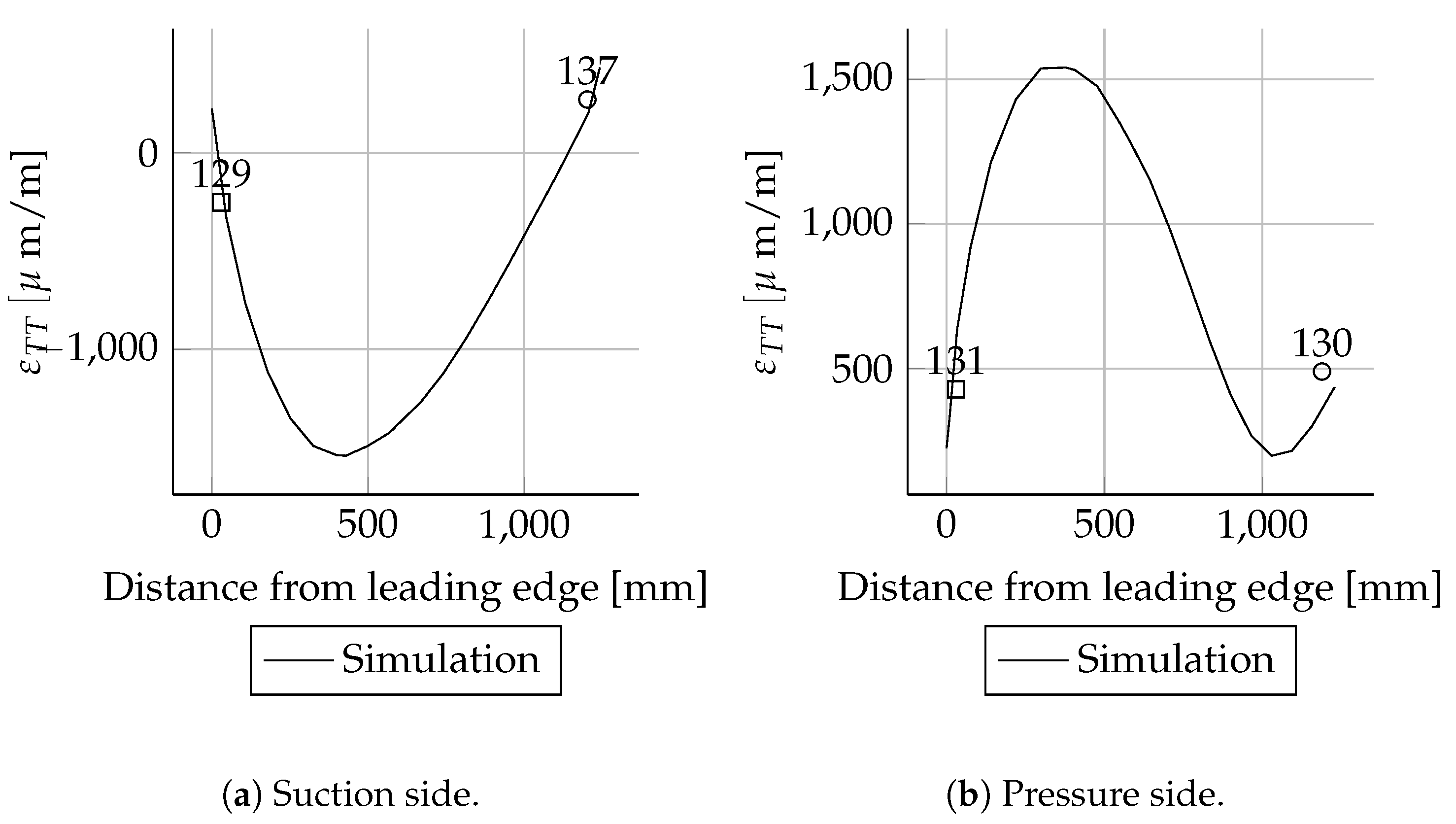
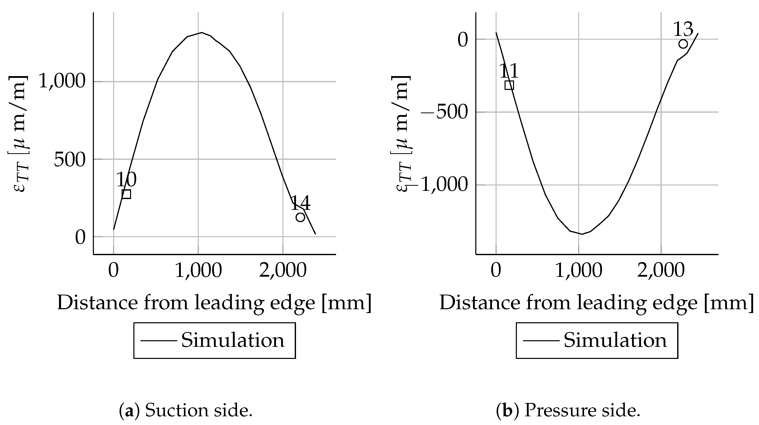
All measured values ${\epsilon }_{TT}$ for the cross-sections at $L=$ 1600, 2700, 11,000, 13,000, 15,000 and 17,000 mm are in good agreement with the simulations. In these cross-sections only the leading and trailing edges were instrumented with strain gauges. Therefore, the cross-sectional circumferential strain distribution is unknown.

Discussion of Mxmin, Mymax and Mymin Results in Relation to Mxmax

The results for the other three load cases are only discussed briefly. The overall behaviour is equal to the Mxmax load case. The results for Mxmin (cf. Figure 4b) are shown in Appendix D.2. As in the Mxmax load case, the Mxmin simulation and the experiment showed the highest strains at leading and trailing edges, as expected; cf. Figure A15 for the mechanical strains of the spar caps and Figure A16, Figure A17, Figure A18, Figure A19, Figure A20, Figure A21, Figure A22, Figure A23, Figure A24 and Figure A25 for the mechanical strains of the leading and trailing edge.

When comparing the load cases Mxmax and Mxmin for the spar caps, a switch in signs for the ${\epsilon }_{LL}$ strain values can be seen; cf. Figure A2a and Figure A15a. This was expected because the rotor blade was rotated by 180° between the two load cases. The overall quality of the numerical result is comparable to the Mxmax load case.

Due to the orientation of the rotor blade in Mymax and Mymin load cases the mechanical strains at the spar caps were higher compared to those at the leading and trailing edges. Both the simulation and the experiment showed this behaviour; cf. Figure A28 and Figure A41 for the mechanical strains of the spar caps and Figure A29, Figure A30, Figure A31, Figure A32, Figure A33, Figure A34, Figure A35, Figure A36, Figure A37 and Figure A38 and Figure A42, Figure A43, Figure A44, Figure A45, Figure A46, Figure A47, Figure A48, Figure A49, Figure A50 and Figure A51 for the mechanical strains of the leading and trailing edges.

For the three load cases, Mxmin, Mymax and Mymin, the absolute deviations were small for most sensor positions. As expected, the relative deviations were higher in areas with small strains than in areas with larger strains. This behaviour can be seen very clearly when comparing the suction side spar cap strains with the pressure side spar cap strain. These are the absolute values for the pressure side. Therefore, the deviations are relatively high. The suction side course matches well in the simulations and experiments. In the case of the pressure side, there are bigger differences close to the root. Besides some exceptions, all measured values ${\epsilon }_{LL}$ and ${\epsilon }_{TT}$ are in good agreement with the simulations.

4.1.4. Torsion—Displacements

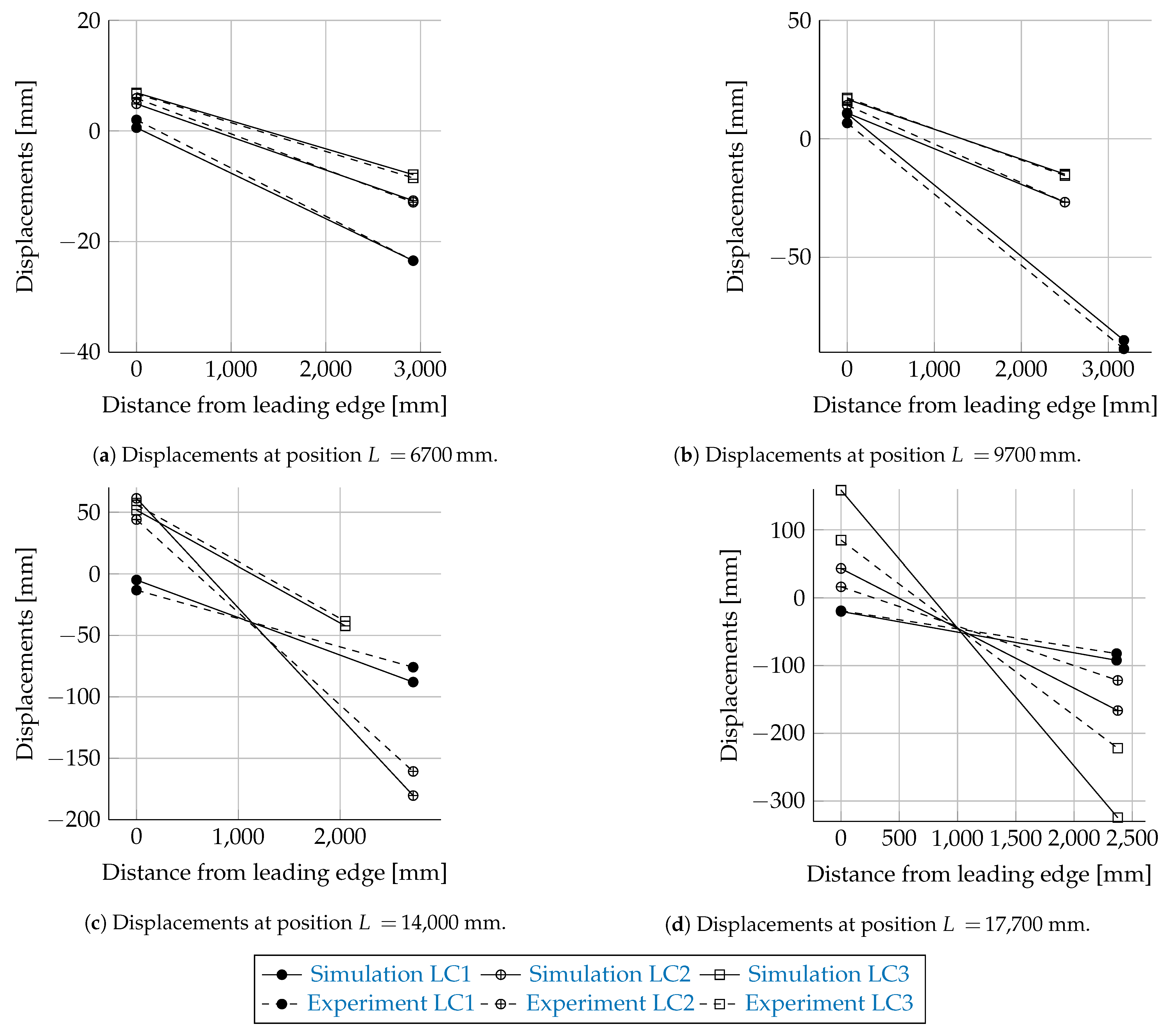
The comparisons of the torsion stiffness measurement (see Section 2.1.2) results and the numerical results are illustrated in Figure 11a–d. Three scenarios (LC1, LC2 and LC3) were measured and simulated. The load vectors for the load cases are given in Table 2. The scenario LC1 is in good agreement for all measurement positions. In this scenario, the error is dominated by the load introduction point $L=$ 9700 $\mathrm{m}$$\mathrm{m}$. As this error is small, the outer radial cross-section errors are small as well.

For scenario LC2 the error is bigger compared to LC1 for the cross-sections $L=$14,000 and $L=$17,700 mm. The numerical model is softer compared to the tested rotor blade, because the angle of rotation (inclination of the curve) is larger.

For scenario LC3 the largest error occurred at $L=$17,700 mm, where the load was introduced. The conclusion is that the rotor blade model was modelled too flexibly at the outer third of the rotor blade. The torsion angles at various positions are given in

Table 6. Torsion angles at various positions.

Position [mm]	LC1 [${}^{°}$]		LC2 [${}^{°}$]		LC3 [${}^{°}$]
	Exp.	Sim.	Exp.	Sim.	Exp.	Sim.
6700	−0.55	−0.64	$-0.36$	−0.46	−0.29	−0.39
9700	−1.71	−1.74	−0.94	−1.29	−0.75	−1.08
14,000	−1.32	−1.74	−4.32	−5.08	−2.64	−4.25
17,700	−1.52	−1.74	−3.3	−5.09	−7.42	−11.78

. It must be noted that for the LC1 load case all angles determined at positions $L>$ 9700 $\mathrm{m}$$\mathrm{m}$ have the same value. The reason is that no additional load was applied further away and no additional torsion deformation was induced.

4.1.5. Torsion—Strains

The strain distributions for the intensively instrumented cross-sections $L=$ 5000 and $L=$ 8000 $\mathrm{m}$$\mathrm{m}$ are given in Appendix D.6 for all three load cases LC1LC3. Most of the numerical results are not in good agreement with the experimental data. Generally speaking, most of the strains were lower than 100 $\mathsf{\mu }$$\mathrm{m}$/$\mathrm{m}$. As in the bending cases, these small strains were more sensitive against minor orientation and placement errors. For larger strains above 100 $\mathsf{\mu }$$\mathrm{m}$/$\mathrm{m}$, the curves are in better agreement and fit best for Figure A54b and Figure A56a,b for the first load case LC_1. For LC_3, Figure A62b and Figure A64b show good agreement between simulation and measurements.

4.2. Validation of the Mass Distribution

The mass of the first produced rotor blade (blade 1) was measured before testing at the test bench. The masses of the other three rotor blades (blade 2, 3 and 4) were measured after the finish. The reference finite element model did not include specific parts, such as

i

Varnishing ( 14 $\mathrm{k}$$\mathrm{g}$);

ii

Mounting bolts ( $74.1$ $\mathrm{k}$$\mathrm{g}$);

iii

Torsion sensor ( $4.8$ $\mathrm{k}$$\mathrm{g}$);

iv

Blade tip ( $2.2$ $\mathrm{k}$$\mathrm{g}$);

v

Trimming mass in balancing chamber ( 6 $\mathrm{k}$$\mathrm{g}$);

vi

Lightning protection cables ( $24.3$ $\mathrm{k}$$\mathrm{g}$);

vii

Reflector system ($110.3$ $\mathrm{k}$$\mathrm{g}$).

The mass of rotor blade 1 has to be reduced by $119.5$ $\mathrm{k}$$\mathrm{g}$, because the rotor blade was not finished (excluding points i, iv and v). The masses of rotor blades 2–4 were measured after the finish, and their mass has to be reduced by $135.7$ $\mathrm{k}$$\mathrm{g}$ to be comparable with the finite element model. The mass and the centre of mass of the reference rotor blade in comparison to the measured four wind turbine blades are given in

Table 7. Mass distribution and centre of mass.

Type	Reference FE Blade	Reference FE Blade with Bolts	Blade 1	Avg. Blade 2–4
Mass [kg]	1745.4	-	1673.5 ± 45 ${}^1$	1795.3 ${}^2$
Centre of mass [mm]	6759.0	6483.8	6580 ± 200 ${}^3$	6070 ${}^3$

¹ 119.5 kg extra mass has been subtracted from the measured mass. ² 135.7 kg extra mass has been subtracted from the measured mass. ³ Measured with bolts.

. Blade 1 was measured before mounting to the test bench at test facility (no finish). Blades 2–4 were measured at the finisher company. The extra masses were subtracted from the measured values, because they were not included in the reference model. The masses of the model and the built rotor blades had differences of 4.1% for blade 1 and 2.8% for the blades 2–4’s average mass.

The centre of mass measurement of the finite element model and the measurements are in the same order. The effects of the bolts on the centre of mass were tested by including them. It can be seen that the centre of mass was in good agreement with rotor blade 1 with an error of 2.7% without the bolts and 1.4% with bolts. For the finished rotor blades 2–3, the error was 11.4% without the bolts and 6.8% with bolts, respectively.

4.3. Section-Wise Centre of Mass

Blade 1 was cut into sections, as shown in Figure 12. For each section the mass and the centre of mass was measured.

The comparison between the model and the measured results is given in

Table 8. Section-wise measured centre of mass in global coordinates mass per length.

Section	Measurement	Model	Measurement	Model	Measurement	Model	Measurement Mass	Model Mass
[m]	z [m]	z [m]	x [m]	x [m]	y [m]	y [m]	[kg/m]	[kg/m]
0–0.9	0.3	0.2	0.0	0.0	0.086	0.0	391	355
0.9–2.0	1.4	1.4	0.0	0.0	0.0	0.0	130	103
2.0–3.0	2.4	2.4	0.0	0.0	0.075	0.188	117	131
3.0–3.5	3.2	3.25	0.0	0.0	0.131	0.211	119	119
3.5–4.0	3.7	3.74	0.0	0.0	0.162	0.221	112	134
4.0–5.2	4.5	4.60	0.0	0.0	0.218	0.220	104	105
5.2–6.5	5.7	5.84	0.0	0.0	0.229	0.227	94	103
6.5–8.5	7.4	7.48	0.0	0.0	0.184	0.210	84	96
8.5–9.5	8.9	8.99	0.0	0.0	0.146	0.191	75	84
9.5–10.5	9.8	9.99	0.0	0.0	0.131	0.181	72	77
10.5–11.5	10.8	10.99	0.0	−0.05	0.123	0.166	68	73
11.5–12.5	11.9	11.99	−0.1	−0.08	0.114	0.155	62	67
12.5–16.0	14.0	14.13	−0.21	−0.21	0.109	0.152	53	59
16.0–16.5	16.1	16.24	−0.38	−0.40	0.1	0.157	50	44
16.5–17.5	-	16.99	-	−0.49	-	0.173	-	44
17.5–19.0	18.0	18.10	−0.63	−0.65	0.2	0.27	31	24
19.0–20.0	19.4	19.38	−0.87	−0.87	0.43	0.45	15	10

. The coordinates are given in global rotor blade coordinates. The results of the numerical model and the measurements are in agreement. The main discrepancy was present due to manufacturing problems at rotor blade 1. As shown in Figure 12a the adhesive joint between the spar cap and the shear web flange was not filled. Therefore, the mass distributions between the numerical model and the real rotor blade were different. It must be noted that the section 16.5–$17.5$ $\mathrm{m}$ was not measured because the part was missing.

4.4. Validation of Eigendynamics

4.4.1. Solver

As linear eigenvalue solver the Lanczos method [16] was used to perform all modal analyses.

4.4.2. Eigendynamics

Two configurations were analysed and measured. A clamped configuration and a free–free configuration. In this paper the eigenmodes were not compared with a Modal Assurance Criterion (MAC) criterion [17]. The data of the eigenfrequencies and eigenmodes are taken from [11], where more detailed analysis of the modes and the experimental setup can be found.

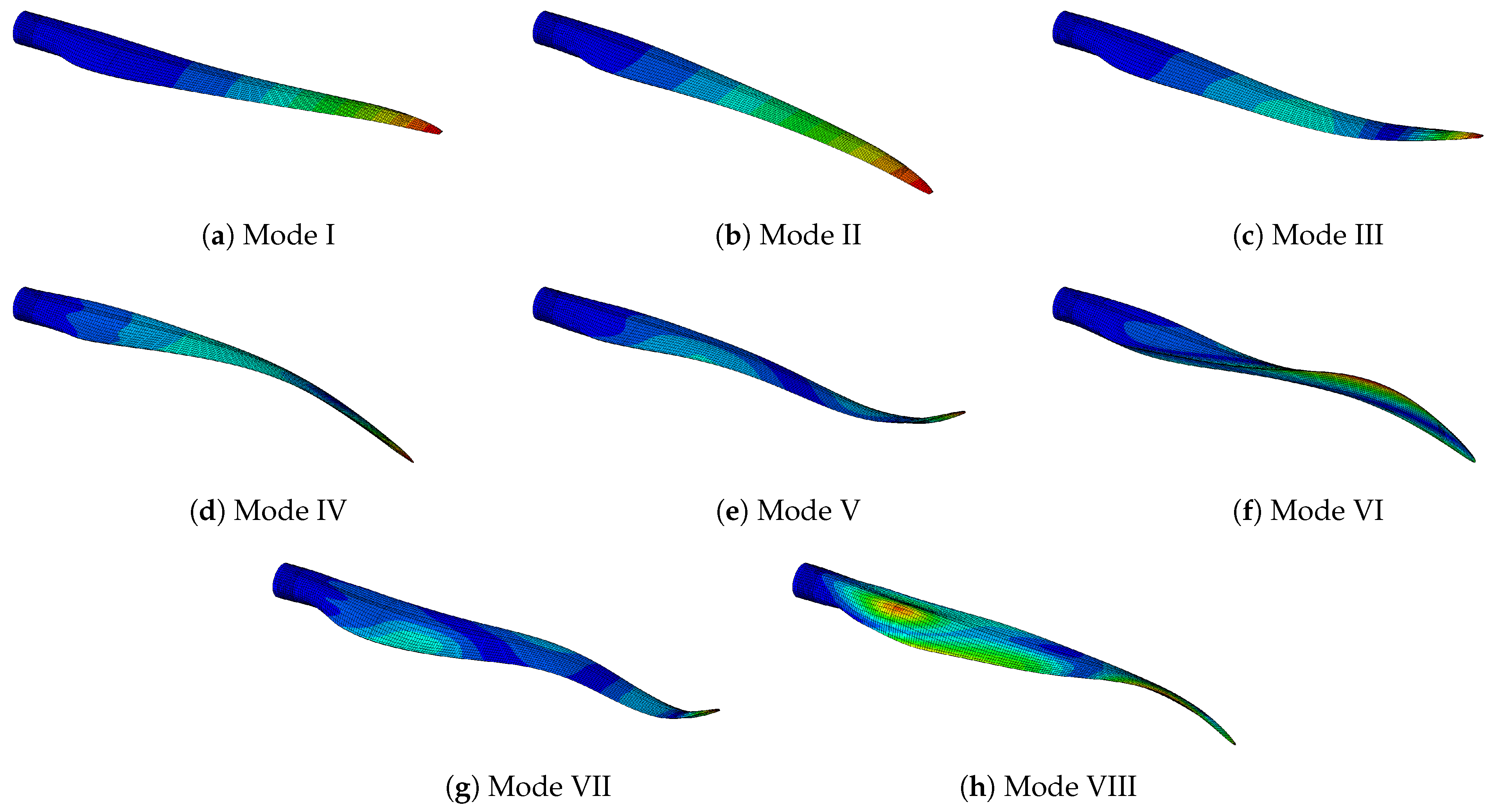
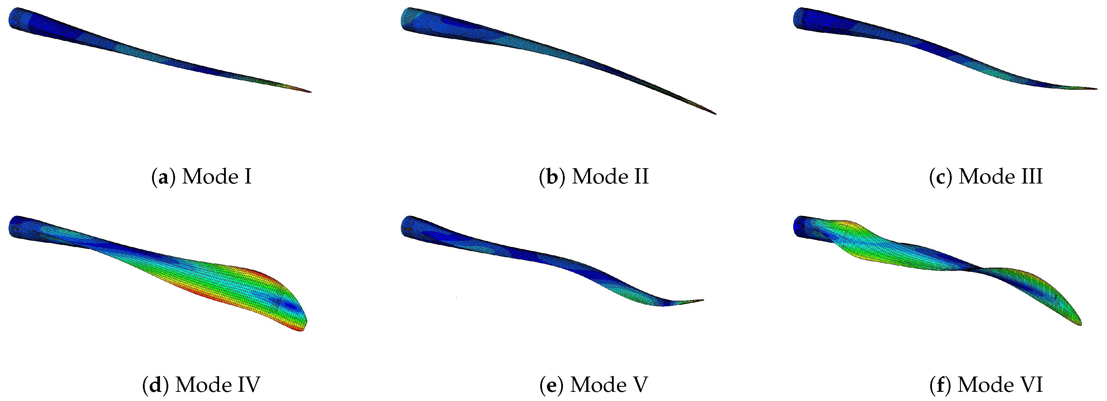
The first 8 eigenfrequencies of the clamped rotor blade are given in

Table 9. Eigenfrequencies of the clamped rotor blade simulated in Abaqus.

Number	Type	Reference Model	Design Model	Experiments	Error R/D	Error R/E
		[Hz]	[Hz]	[Hz]	[%]	[%]
1	Bending flapwise	2.33	2.41	2.2	−3.3	5.9
2	Bending edgewise	3.09	3.43	3.07	−9.9	0.65
3	Bending flapwise	6.85	7.4	6.84	−7.4	0.15
4	Bending edgewise	10.38	11.49	10.86	−9.6	−4.4
5	Bending flapwise	13.28	14.25	13.57	−6.8	−2.14
6	Torsion	16.45	18.78	17.82	−12.4	−7.69
7	Bending flapwise	20.70	21.99	21.66	−5.8	−4.43
8	Bending flapwise	21.25	-	22.37	-	−5.01

. The results of the reference model are compared to the design model [18] (R/D) and the experimental data (R/E). The comparison between the simpler design model lead to errors lower 10% except the torsion mode. As the frequency error was too large for the analysis some of the masses excluded for the mass comparison were added to the model; see Section 4.2. This includes the torsion sensor (iii), wind turbine blade tip (iv), trimming mass in balancing chamber (v) and the reflector system (vii). The bolts does not influence the clamped rotor blade and were not in place for the free–free experiment. The varnishing was not done for the actual rotor blade tested in the test bench. The mass of the lightning protection system was excluded.

The errors between the reference model and experiment without any model updating for all bending eigenmodes is lower than 6%. However with an error greater 5% it would not be conform to certification requirements. For the first flapwise bending mode the difference can be found due to lower tip masses in the finite element model compared to the real rotor blade; cf. Table 8. This leads to a reduction in the eigenfrequencies. The first torsion mode has a difference of −7.6% and it is assumed that the stiffness of the root section is underestimated by the finite element model. The eigenmodes are shown in Figure 13.

For the free–free configuration the first 6 non-rigid body eigenfrequencies are shown in

Table 10. Eigenfrequencies in free–free configuration of the rotor blade simulated in Abaqus.

Number	Type	Reference Model [Hz]	Experiments [Hz]	Error R/E [%]
1	Bending flapwise	5.07	4.8	5.63
2	Bending edgewise	9.97	10.3	−3.2
3	Bending flapwise	12.03	11.99	0.33
4	Torsion	16.9	16.85	0.3
5	Bending flapwise	20.89	20.9	0.01
6	Torsion	25.95	27.98	−7.26

. Analysis results of the design model do not exist and are therefore not compared. The eigenmodes are shown in Figure 14. Except for the second torsion mode all errors are lower than 10%. It must be noted that the first torsion mode has an error of 0.3%. This is an indication that the root area has been modelled with insufficient stiffness or the mass distribution is incorrect as stated for the clamped configuration [10].

Comparing both analysis it can be seen, that the torsion frequencies differ stronger for the clamped configuration. The reason might be in a stiffer root section of the real rotor blade. This leads for the clamped configuration to higher frequencies compared to the free–free configuration. The mass distribution for the torsion modes seems to be okay. Differences of the center of gravity between the finite element model and the real rotor blade would not have a massive impact, because the pre bend over compensate this effect.

5. Discussion

The general findings of the study will be discussed below. For the static loads, it can be seen that the global deformations are in good agreement between the simulation and the experiment. This applies to all bending and torsion load cases. For the torsional loads, the largest deviation is in the outer area of the rotor blade. There are two main reasons. First, the introduction of a pure torsional load is difficult. Second, minor deviations due to manufacturing have a culmunative effect on the errors in the direction of the blade tip.

The error between the simulation and experiment of the mechanical strains for all load cases are usually larger compared to the errors in the displacements. The reason for this can be found in the positioning of the strain gauges and in manufacturing deviations. The position of the strain gauges refers to a local coordinate system measured on the blade. The origin is the nose of the rotor blade for the instrumented profile. The finite element model refers to the aerodynamic shape. The real manufactured blade without finish does not correspond to this everywhere. This means that the distance from the nose to a specific sensor can differ in the range of centimeters. Thus, there are certain differences between real positioning and model-side positioning, because a pre finished blade was tested.

As stated manufacturing errors influence the strain measurements as well. The fibre placement usually does not correspond exactly to the orientation assumed in the finite element model. This can lead to errors in the strain measurement due to the locally different stiffness.

The argumentation on the effects of production-related deviations is supported by the mass distribution. There, it can be seen from the measurement that there are deviations in the centers of gravity. It is to be expected that these are in the same order of magnitude for the stiffnesses. This, of course, affects the inherent dynamics of the rotor blade. There, especially the lower natural frequencies are strongly subjected to errors and would fail the certification. To improve the results, the manufacturing deviations would have to be taken into account in the FEM model. Depending on the available database, this can be achieved by using measurement data from the real rotor blade or by automatic model updating.

Two very important issues were identified during the validation process

• Experimental and computational engineers do not speak exactly the same language. Therefore, a close communication is key, because a lot of information which is not important for the experimental engineer is very important for the computational engineer, vice versa.
• A good documentation of the experiment with many fotos are very important. This holds especially for seemingly trivial information.

6. Conclusions

The paper presents a finite element model of a 20 $\mathrm{m}$ wind turbine blade and its validation. The finite element model was created using manufacturing specifications. The validation was based on mass distribution data and static and modal test data. The static test data were composed of displacement and strain measurements. The validation indicated that the difference between simulated and measured displacements for all bending tests was less than 10%. For the torsion tests, the resulting rotor blade rotations were in good agreement for most of the tests. The largest differences were seen in the third torsion test, where the load was applied in the outer area.

However, except for the spar caps, simulated strains were in good agreement with the measured strains. The reason for that was a faulty instrumentation of the experimental setup. The natural frequencies matched in some cases with an error below 5% and would conform to certification requirements. In other cases (first flapwise mode; first torsion mode) the error was above that, which does not work with the certification requirements. Further investigation of, e.g., clamping and mass distribution impacts, has to be done. The mass distribution also matches the experimental data. The finite element model was translated into Abaqus, Ansys and Nastran, and is provided as a reference model. The dataset includes also the measurement data used, and python scripts as easy-access solutions for other researchers [7].

References

- Serrano-Gonzalez, J.; Lacal-Arantegui, R. Technological evolution of onshore wind turbines—A market-based analysis. Wind Energy 2016, 19, 2171–2187. [Google Scholar] [CrossRef]
- Zalkind, D.S.; Ananda, G.K.; Chetan, M.; Martin, D.P.; Bay, C.J.; Johnson, K.E.; Loth, E.; Griffith, D.T.; Selig, M.S.; Pao, L.Y. System-level design studies for large rotors. Wind Energy Sci. 2019, 4, 595–618. [Google Scholar] [CrossRef]
- Veers, P.; Dykes, K.; Lantz, E.; Barth, S.; Bottasso, C.L.; Carlson, O.; Clifton, A.; Green, J.; Green, P.; Holttinen, H.; et al. Grand challenges in the science of wind energy. Science 2019. [Google Scholar] [CrossRef] [PubMed]
- Zhou, H.; Dou, H.; Qin, L.; Chen, Y.; Ni, Y.; Ko, J. A review of full-scale structural testing of wind turbine blades. Renew. Sustain. Energy Rev. 2014, 33. [Google Scholar] [CrossRef]
- Peeters, M.; Santo, G.; Degroote, J.; Paepegem, W.V. Comparison of Shell and Solid Finite Element Models for the Static Certification Tests of a 43 m Wind Turbine Blade. Energies 2018, 11, 1346. [Google Scholar] [CrossRef]
- Fingersh, L.; Johnson, K. Controls Advanced Research Turbine (CART) Commissioning and Baseline Data Collection; Technical Report; National Renewable Energy Laboratory: Denver, CO, USA, 2002. [Google Scholar]
- Willberg, C. Smartblades 2 Finite Element Reference Rotorblade Model. 2020. Available online: https://zenodo.org/record/3628356#.YILQpVARWMo (accessed on 22 April 2021).
- Haller, B.; Noever-Castelos, P. Full Scale Blade Test of a 20 m Wind Turbine Blade within the SmartBlades2 Project. 2021. Available online: https://zenodo.org/record/4605409#.YILPVlARWMo (accessed on 22 April 2021).
- IEC 61400-5:2020. Wind Energy Generation Systems—Part 5: Wind Turbine Blades; Standard; International Electrotechnical Commission: Genf, Switzerland, 2020. [Google Scholar]
- Knebusch, J.; Gundlach, J.; Govers, Y. A systematic investigation of common gradient based model updating approaches applied to high-fidelity test-data of a wind turbine rotor blade. In Proceedings of the EASD Procedia, EURODYN 2020—XI International Conference on Structural Dynamics, Athens, Greece, 23–26 November 2020; pp. 2159–2174. [Google Scholar] [CrossRef]
- Gundlach, J.; Govers, Y. Experimental modal analysis of aeroelastic tailored rotor blades in different boundary conditions. IOP Conf. Ser. J. Phys. Conf. Ser. 2019. [Google Scholar] [CrossRef]
- Heydlauff, W. Materialspezifikation der Faserverbundwerkstoffe für das Rotorblatt IWES20.0—Testbench Version—Rev. 2.0; Technical Report; Aero Dynamik Consult—Ingenieurgesellschaft mbH: Neuhausen auf den Fildern, Germany, 2018. [Google Scholar]
- Jones, R.M. Mechanics of Composite Materials; Tayler & Francis Inc.: Milton Park, UK, 1999. [Google Scholar]
- Jensen, F.M. Ultimate Strength of a Large wind Turbine Blade; Risø DTU: Roskilde, Denmark, 2008; ISBN 978-87-550-3634-5. [Google Scholar]
- Keil, S. Technology and Practical Use of Strain Gages with Particular Consideration of Stress Analysis Using Strain Gages: With Particular Consideration of Stress Analysis Using Strain Gages; Wilhelm Ernst & Sohn, Verlag für Architektur und technische Wissenschaften GmbH & Co. KG: Berlin, Germany, 2017. [Google Scholar] [CrossRef]
- Parlett, B.N.; Nour-Omid, B. Towards a black box Lanczos program. Comput. Phys. Commun. 1989, 53, 169–179. [Google Scholar] [CrossRef]
- Pastor, M.; Binda, M.; Harcarik, T. Modal Assurance Criterion. Procedia Eng. 2012, 48, 543–548. [Google Scholar] [CrossRef]
- Heydlauff, W. Stress Analysis and FE-Calculation of the Rotorblade IWES20.0—Revision 13; Technical Report; Aero Dynamik Consult—Ingenieurgesellschaft mbH: Neuhausen auf den Fildern, Germany, 2017. [Google Scholar]
Figure 1.
Experimental setup for load case Mymax by Fraunhofer IWES [
8].
Figure 2.
Top view of positions of strain gauges and definition of the load frames (LF 1–4) [
Figure 3.
The root jig of the test bench [
10].
Figure 4.
Rotor blade orientation for all bending and torsion load cases. (a) Blade orientation during load case Mxmax. (b) Blade orientation during load case Mxmin. (c) Blade orientation during load case Mymax and torsion tests. (d) Blade orientation during load case Mymin.
Figure 5.
Finite element model of the 20 rotor blade.
Figure 6.
Reference planes and stacking directions.
Figure 7.
Suction side of the rotor blade to illustrate assumptions made at the trailing edge (black circle).
Figure 8.
Visualisation of the shell and solid element distribution in a cross-section. (a) Visualisation of the shell and solid element distribution. (b) Visualisation of the virtual thickness of the shell elements.
Figure 9.
Displacements for all bending load cases.
Figure 10.
Definition of a strain gauge rosette.
Figure 11.
Displacements for all torsion load cases.
Figure 12.
Comparison of as-built structure and finite element model. (a) Cross-section of the wind turbine rotor blade after cutting. (b) Cross-section of the wind turbine blade in the finite element model.
Figure 13.
Eigenmodes of the clamped rotor blade simulated in Abaqus.
Figure 14.
Eigenmodes of the free–free configuration of the wind turbine blade simulated in Abaqus.