Article

Weather-Driven Scenario Analysis for Decommissioning Coal Power Plants in High PV Penetration Grids

by
Samuel Matthew G. Dumlao
* and
Keiichi N. Ishihara
Department of Socio-Environmental Energy Science, Graduate School of Energy Science, Kyoto University, Yoshidahonmachi, Sakyo-ku, Kyoto 606-8501, Japan
*
Author to whom correspondence should be addressed.
Energies 2021, 14(9), 2389; https://doi.org/10.3390/en14092389
Submission received: 29 March 2021 / Revised: 16 April 2021 / Accepted: 19 April 2021 / Published: 22 April 2021
(This article belongs to the Special Issue Energy for Sustainable Future)

Abstract

:
Despite coal being one of the major contributors of CO 2 , it remains a cheap and stable source of electricity. However, several countries have turned to solar energy in their goal to “green” their energy generation. Solar energy has the potential to displace coal with support from natural gas. In this study, an hourly power flow analysis was conducted to understand the potential, limitations, and implications of using solar energy as a driver for decommissioning coal power plants. To ensure the results’ robustness, the study presents a straightforward weather-driven scenario analysis that utilizes historical weather and electricity demand to generate representative scenarios. This approach was tested in Japan’s southernmost region, since it represents a regional grid with high PV penetration and a fleet of coal plants older than 40 years. The results revealed that solar power could decommission 3.5 GW of the 7 GW coal capacity in Kyushu. It was discovered that beyond 12 GW, solar power could not reduce the minimum coal capacity, but it could still reduce coal generation. By increasing the solar capacity from 10 GW to 20 GW and the LNG quota from 10 TWh to 28 TWh, solar and LNG electricty generation could reduce the emissions by 37%, but the cost will increase by 5.6%. Results also show various ways to reduce emissions, making the balance between cost and CO 2 a policy decision. The results emphasized that investing in solar power alone will not be enough, and another source of energy is necessary, especially for summer and winter. The weather-driven approach highlighted the importance of weather in the analysis, as it affected the results to varying degrees. The approach, with minor changes, could easily be replicated in other nations or regions provided that historical hourly temperature, irradiance, and demand data are available.

1. Introduction

In 2013, signatories to the Paris Agreement committed to submit a national climate plan to mitigate climate change by reducing greenhouse gas emissions. Subsequently, one of the United Nations’ Sustainable Development Goals, established in 2015, is focused on affordable and clean energy. These two global initiatives have motivated several nations to promote renewable energy sources such as wind, solar, and biomass into their energy mix. As a result, several “green energy transition” initiatives are ongoing in countries such as Germany and Denmark, and subnational jurisdictions such as California, Scotland, and South Australia [1]. Besides these major players, more than 150 countries have national targets for renewable energy in the power sector [2].
The Japanese government recently reiterated its commitment to the projected energy mix for 2030, where fossil fuel-based generation will be reduced to 46%, and renewable energy will comprise 22–24%, of which solar energy will have a 7% contribution [3]. There was a recent influx of solar PV installation mainly driven by the FIT program. The Kyushu region, located on Japan’s western tip, is one of the country’s leading regions in solar PV generation. Relative to the rest of the country, the region has higher solar power potential and cheaper land, which has driven solar power investments. As of early 2021, the region has a total installed capacity of 10 GW, and additional plants, which will increase this capacity further to roughly 16 GW [4] by around 2027, are already approved. The share of solar PV generation has been steadily increasing in the region. In 2017, 2018, and 2019, solar PV generation accounted for 8.5%, 9.2%, and 10.1% of the total yearly generation, respectively. The International Energy Agency (IEA) classifies the impact of variable renewable energy (VRE) on the energy system’s operation into four phases. Japan, as a country, is already in phase 2 where there is a minor to moderate impact on the system operation, whereas Kyushu, as a region, was categorized as phase 3, where VRE determines the operation pattern of the system [5]. This further shows that Kyushu is leading the country in terms of solar PV penetration and is already facing issues ahead of the rest of the country. Kyushu’s situation lends itself as a viable case study in exploring the potential impact of solar energy in reducing CO 2 emissions by replacing traditional energy sources with solar energy.
Coal remains to be the cheapest and most economically stable source of electricity for many countries. However, it is also one of the major contributors of CO 2 , which leads to global warming. Among the G7 countries, Germany (by 2038 [6]), France (by 2023 [7]), the United Kingdom (by 2024 [7]), Italy (by 2025 [7]), and Canada (by 2030 [8]) have presented their coal phase-out plans. Other European Union member countries have also developed their phase-out plans within the next two decades, and Austria and Belgium have already phased-out their coal plants [7]. Nonetheless, removing coal is a significant roadblock to the green energy transition in many countries, and as countries install increasing amounts of renewable energy, it might be time to consider reducing coal in the energy mix. Solar photovoltaics (PV) can be a green alternative to coal. However, the generation profile of solar energy is different from that of coal, which complicates the process of replacing coal with solar energy. Simultaneously, the variability of solar power requires another flexible source. Liquefied petroleum gas (LNG), given its flexibility, is often used to balance the VRE. Given these intertwined variables, it is necessary to understand the potential, limitations, and implications of using solar energy to replace coal, which are currently unclear.
Many countries see LNG as a bridge to a clean energy future that will pave the way for less coal in the energy mix [9]. It is still a fossil fuel, but it produces less CO 2 , which is acceptable for now until a superior technology is available. Due to many countries’ tendency to rely on LNG to reduce their CO 2 emissions, the demand for LNG has steadily been increasing, which threatens its supply and price. Shell reported in their LNG Outlook 2020 that global demand for LNG increased by 12.5% to 359 million tons in 2019, which they attributed mainly to the role of LNG in the low-carbon energy transition [10]. It has been reported that the price of LNG increased in October 2020 in anticipation of a colder winter in East Asia [11]. This shows the volatility of LNG’s supply and price on the global market, which presents another factor for consideration in the analysis, since solar energy production needs LNG to a certain extent.
Aside from the potential CO 2 reduction benefits, reducing coal capacity could also reduce solar curtailment experienced by grids with high PV penetration. Kyushu started to suffer from curtailment in October 2018, which was explored in a previous study [12]. Several studies have also explored this recent issue in Kyushu. Bunodiere and Lee [13] explored several scenarios to mitigate solar curtailment in Kyushu using a logic-based forecasting method and concluded that reducing the region’s nuclear capacity will reduce curtailment. However, in their approach, they considered coal and LNG as thermal generators as a whole due to data limitations. A coal station behaves like a nuclear plant, since these two technologies are considered baseload generators. By treating coal as separate from LNG and as a baseload generator, it could also be said that coal could reduce curtailment. Although Japan initially used their pump hydro energy storage (PHES) to improve the flexibility of nuclear power plants [14], it is now used to store excess solar electricity generation. Li et al. [15] conducted a techno-economic assessment of large-scale PV integration with PHES and concluded that the PHES could effectively absorb some of the surplus PV production and could maintain low generation cost by using the surplus production. Since the available data regarding power generation in the region aggregate coal and LNG together, the understanding of coal generation in the energy balance is limited.
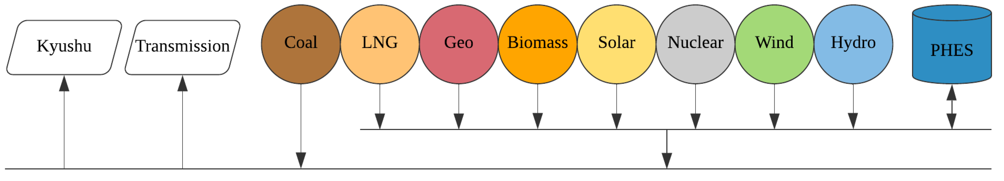
In order to fully understand the optimal conditions for coal, solar, and LNG production, it is necessary to conduct a power flow analysis to evaluate the impact of investing in more solar PV for driving coal decommissioning. This analysis will provide additional information about the energy balance, including information about solar power generation and curtailment, which are difficult to estimate. By gathering the generators’ capacity and generation profiles and the demand profiles, the optimization can calculate the hourly energy balance and minimize the necessary coal capacity and generation. This insight provides the necessary understanding of the potential and limitations of solar energy in regard to replacing coal. However, to ensure the robustness of the analysis and the recommendation, the demand and solar power generation’s stochasticity must be considered. It will be challenging to recommission a decommissioned plant due to an unforeseen circumstance; thus, careful analysis is necessary to account for potential variations.
Replacing part of coal’s electricity production with solar electricity production, coupled with LNG electricity production, is a subset of the generation expansion planning (GEP) problem. Koltsaklis and Dagoumas [16] wrote a review article exploring the state-of-the-art generation expansion planning where they listed seven challenges to the GEP problem. One of the mentioned challenges is rooted in the risks involved in GEP. They enumerated several potential sources of risks and categorized them according to economic, political, regulatory, environmental, technical, social, and climate categories. Ioannou et al. [17] reviewed the risk-based methods for sustainable energy system planning and categorized the risks in the same manner. They identified seven risk-based methods: mean-variance portfolio theory, real option analysis, Monte Carlo simulation, stochastic optimization technique, multi-criteria decision analysis, and scenario analysis.
Santos et al. [18] conducted a study to identify uncertainties in the electricity system and demonstrated the corresponding impacts on the energy mix through scenario analysis. Their results highlighted that climate uncertainty represents primary risk sources for VRE, since it dictates the system’s power generation. A review on the energy sector vulnerability to climate change [19] summarizes the authors’ contributions on climate and energy, and they noted that climate change could affect variables that influence electricity generation from photovoltaics and concentrated solar power. The review highlighted that global solar radiation has increased in southeastern Europe [20] and decreased in Canada [21]. They also highlighted that power output calculations should account for air temperature, since it impacts the solar cell’s efficiency [19].
Ioannou et al. [17] noted that energy planning has extensively used stochastic optimization techniques, and the stakeholder’s motivation mainly drives the constraints. They also mentioned that the Monte Carlo simulation has many advantages, but it requires considerable data inputs to create probability density functions. Alternatively, scenario analysis evaluates the risks by creating potential future developments that range from the worst-case to the best-case scenario, which could then cover all the possible risks in the analysis. As highlighted by several authors [18,19,20,21], climate, and by extension weather, must be considered in modeling solar energy generation. Factors such as the changing solar irradiance and ambient temperature could influence solar panels’ variability and efficiency.
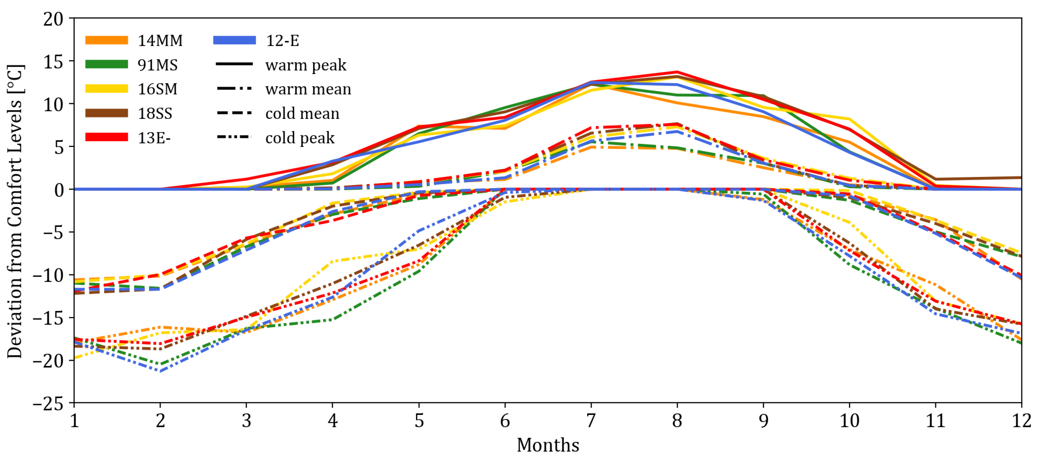
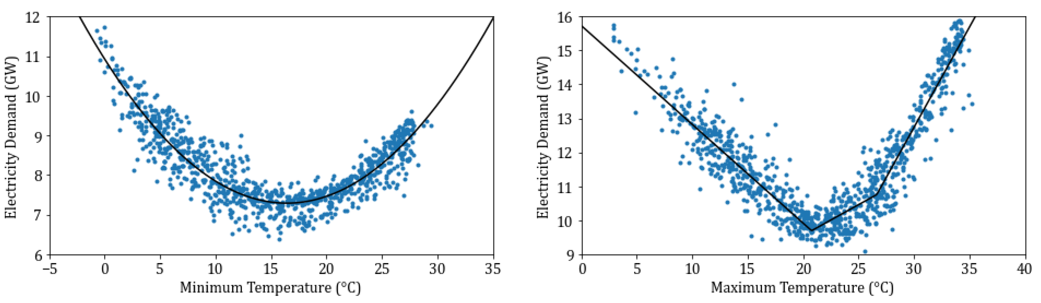
By carefully identifying the test cases, scenario analysis is sufficient for ensuring the robustness of the analysis. The initial problem is then rooted in creating the scenarios representing the worst case, the best case, and the cases in between. The weather data analysis can provide the representative years that fit the scenario targets, such as warm summers, colder winters, extreme summers, and extreme winters. Although such data are limited, datasets could be synthesized based on the historical relationship between temperature and demand. Solar generation could be calculated from the irradiance and ambient temperature data. The robustness of the analysis and recommendation can be addressed by combining scenario analysis and past weather data.
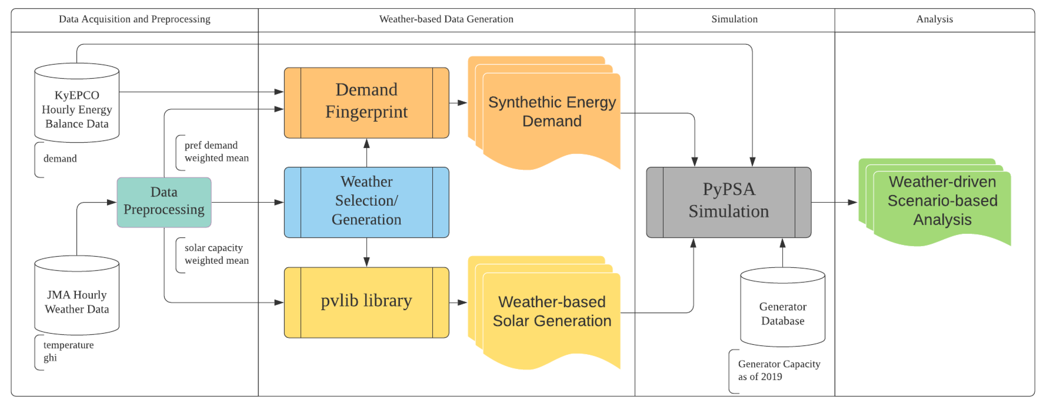
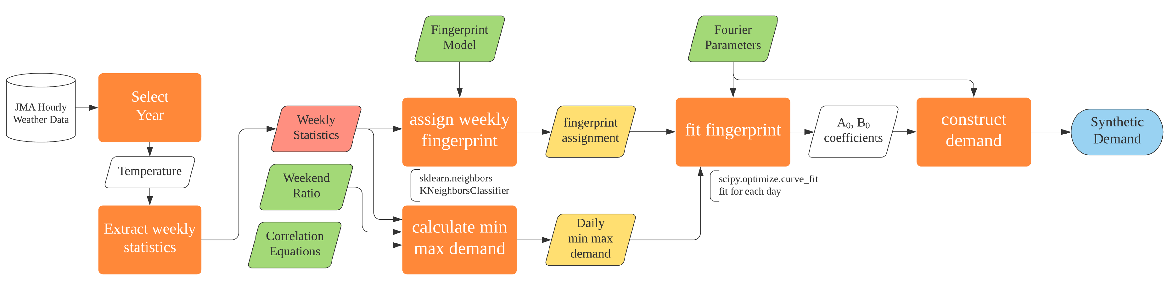
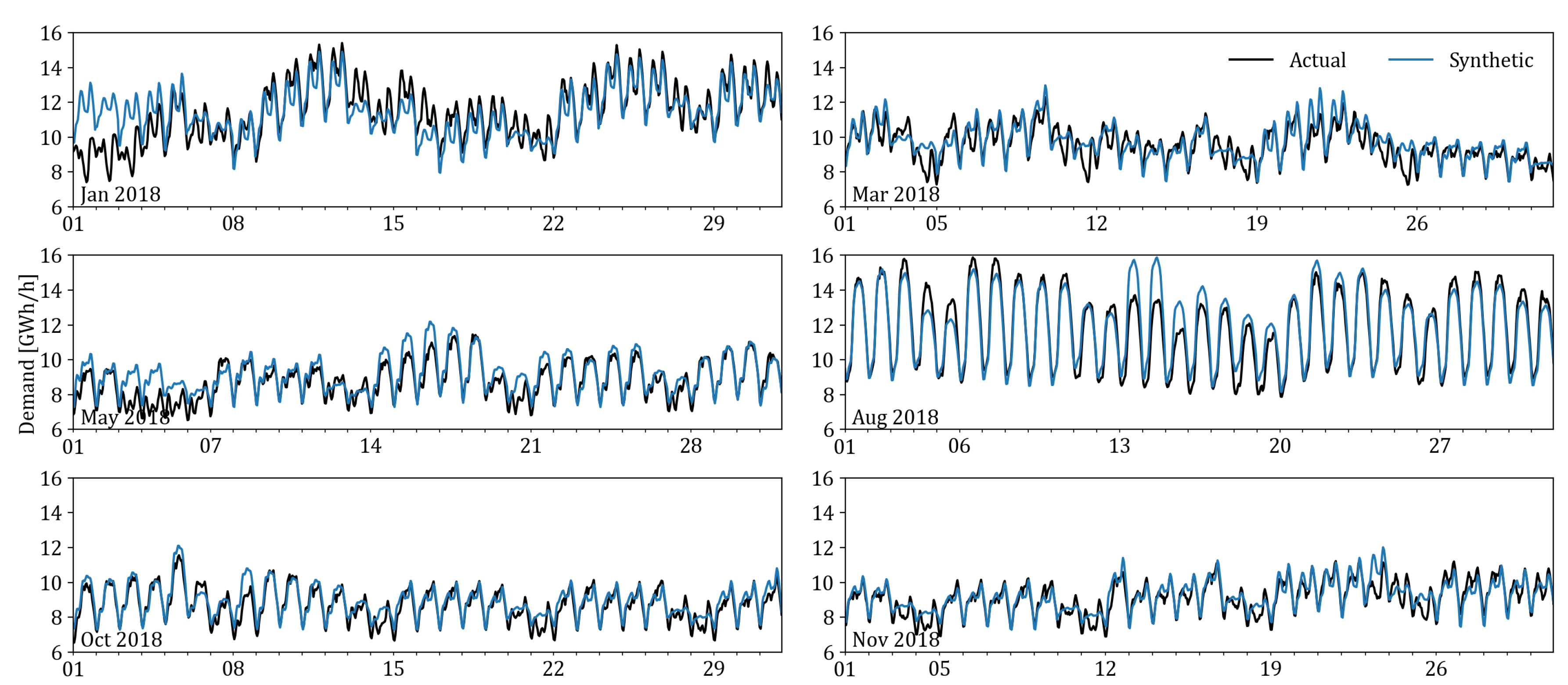
Therefore, in this study, an hourly power flow analysis was conducted to understand the potential, limitations, and implications of using solar energy as a driver for decommissioning coal power plants. Understanding these factors can provide the necessary recommendations and precautions for energy planners. Since LNG scarcity is anticipated, LNG quota is one of the primary constraints. In order to ensure the robustness of the results, this study presents a straightforward weather-driven scenario generation that utilizes historical weather and electricity demand data processed through machine learning algorithms to generate scenarios that account for weather variations. Through the weather-driven approach, the study aims to reveal the impact of yearly variations in the factors that must be considered for long-term planning that reduce CO 2 emissions while ensuring grid reliability. The Kyushu region in Japan was used as a case study since (a) it is continuously increasing its solar capacity, (b) it has a fleet of coal power plants older than 40 years old ready for decommissioning, and (c) it has enough LNG power plant capacity to support the initial transition.
The code for the weather-driven approach used in this study is available through a public GitHub repository [22], where most of the code and diagrams used in this paper are documented in jupyter notebooks. The approach, with minor changes, could easily be replicated in other nations or regions provided that historical hourly temperature, irradiance, and demand data are available.
Section 2 discusses the methodology for the weather-driven approach, including data and data processing, weather-based data generation, and hourly simulation. The results are then presented in Section 3, and the implications are discussed in Section 4. Finally, the conclusions are drawn in Section 5.

2. Methodology

The overview of the proposed weather-driven approach can be seen in Figure 1, where it is divided into four stages. First, data were collected from Kyushu Electric Power Company (KyEPCO) [4] and Japan Meteorological Agency (JMA) [23] and were pre-processed to fit the intended applications. The weather-based data generation has three components. A weather selection metric was designed based on comfort-levels to identify the years that could represent the scenarios in the region. The p v l i b Python library [24] was used to calculate the photovoltaic systems’ generation under various weather conditions. A demand fingerprint was developed to generate synthetic demand for the selected years. These synthetic data were then used as input to the hourly power flow optimization done in Python for Power System Analysis (PyPSA) [25]. Finally, the simulation results were analyzed.

2.1. Data and Data Pre-Processing

2.1.1. Energy Demand

The energy data were collected from Kyushu Electric Company [4], where the hourly information about generation, transmission, and demand is published since April 2016. The data also include curtailment information for both solar and wind power. Transmission and pump hydro energy storage (PHES) could be positive or negative. For transmission, negative values represent energy export while positive values indicate electricity import. For PHES, negative and positive values represent the charging and generation phases, respectively. Although the data until December 2020 are already published, only data until March 2019 were used in the study since this represents four full fiscal years.
As seen in Figure 1, the energy data are used in both the demand fingerprint and simulation phase. Only the demand data were necessary for the demand fingerprint, while the other hourly data were used as parameters for the other generations and PHES.

2.1.2. Temperature and Irradiance

The temperature and irradiance data were collected from the Japan Meteorological Agency (JMA) [23], where the hourly weather data are published since 1946. For this study, 30 years of data were collected from 1990 to 2019 to serve as reference weather scenarios. A representative temperature was collected from each of the major cities’ weather stations, as shown in Table 1.
In order to represent the mean temperature and mean irradiance in the region, solar-capacity-weighted mean and monthly-demand-weighted mean were used for the solar generation calculation and demand generation, respectively. Using the consolidated data from [26], Table 2 shows the shares of the solar PV installation in Kyushu since 2012 and the shares in 2019 were used as the reference for the solar-capacity-weighted mean temperature and irradiance. The Ministry of Economy, Trade, and Industry (METI) publishes each prefecture’s monthly energy demand since April 2016 [27]. Table 3 shows the mean of each prefecture’s shares from 2016 until 2019. These values were used to calculate the monthly-demand-weighted temperature mean used in the demand fingerprint.
The solar capacity ratio was used for the solar power generation calculation because the power generation’s distribution is influenced by the distribution of the capacity. It is necessary to use this weighted mean because the temperature where more solar panels are installed should have a more significant representation in the temperature used in the solar generation calculation. However, the temperature where there is greater demand should have more influence on the temperature used for demand calculations.

2.2. Weather-Based Data Generation

2.2.1. Representative Weather Selection

Since the scenarios are weather-driven, it is necessary to identify the years representing the various scenarios in the region. With this in mind, a metric system was created based on the notion that comfortable temperature levels are between 18 and 22 °C. Under 18 °C, people will start using their heaters, and above 22 °C, they will start using their air-conditioners.
Therefore, the metric system considers the mean and peak deviations per month from these values. Since the focus is to cover extreme cases, the years were ranked based on the summer-warmness and winter-coldness. Based on the rankings, six years were selected, as seen in Table 4. The frequency of occurrence was calculated based on the highest R 2 compared to the representative year from 1990 to 2019. The legends are used mainly in the figures in the results section.
It can be seen in Figure 2 that around August, 2013 has the highest peak and mean positive temperature deviation, while around February, 2012 has the highest peak and mean negative temperature deviation as intended by the sampling. 2014 has the lowest deviation overall since it is the lowest in summer and in the winter. The other representative years fall between these extreme cases.

2.2.2. Weather-Based Solar Generation

The weather-based solar power generation calculation was mainly based on the TMY to power tutorial written by the developers of p v l i b [28]. Since the approach requires both the direct-normal irradiance (DNI) and diffuse horizontal irradiance (DHI), and JMA only provides the global horizontal irradiance (GHI), the built-in function p v l i b . i r r a d i a n c e . e r b s was used to estimate the DNI and DHI. The Erbs model [29] estimates the diffused fraction of GHI to calculate DHI and uses the solar zenith to calculate DNI. By providing the timezone, longitude, latitude, and altitude data along with the hourly GHI data from JMA, the DNI and DHI were calculated using p v l i b ’s built-in functions. Besides the irradiance data, the power generation calculation also requires temperature data to account for the impact of temperature on solar cells’ efficiency. The solar-capacity-weighted mean was used for both the GHI and temperature since the solar power generation distribution is proportional to the generation capacity of each prefecture. Subsequently, the power generation values of a 208 W Kyocera Solar Panel and an ABB Micro 250 W micro-inverter were calculated using p v l i b . p v s y s t e m . s a p m and p v l i b . i n v e r t e r . s a n d i a . The resulting hourly annual generation was scaled by 208 W to represent the maximum power output for PyPSA.

2.2.3. Demand Fingerprint and Synthetic Demand Generation

Figure 3 shows the creation of the four parameters necessary to generate energy demand. The first two swim lanes in the flowchart show the identification of the cluster. Initially, the goal was to extract a demand shape or fingerprint from the data. Since human behavior through weekly routines greatly influences the demand, the energy demand data were split into weekly samples. The peaks and troughs of the demand patterns were identified to emphasize the demand’s fingerprint. This process entailed moving the peaks and troughs to the following hourly locations: 0, 3, 6, 15, 18, 21, and 24, since it was discovered that the peaks and troughs occur at these times depending on the season. Actual values were selected for 9, 11, 12, and 13, since these values represent the midday demand dip that occurs due to the Japanese lunch hour, which is noticeable yearlong. After the alignment, since the goal was to extract the fingerprint, the demand’s magnitude was scaled using z-transform. The resulting scaled value was then used as input to an FFT transform to extract the frequency components that comprise the fingerprint. Only the daily variations (multiples of 7 Hz) were selected as features for the clustering algorithm to reduce the noise. These feature values were scaled using z-transform to reduce the magnitude in the distance calculation.
These features were then clustered using the Kmeans algorithm through the s k l e a r n . c l u s t e r . K m e a n s method of the s k l e a r n Python library. Several values of K were explored, and through experimentation K = 5 was identified as the number of clusters that could explain the data. The clusters’ fingerprints are shown in the inset of Figure 4. Once these clusters were identified, the weekday datasets were combined for each cluster, and another FFT transform was done to extract the Fourier parameters necessary to represent the waveform. Combining the datasets, after clustering, emphasized the pattern for each cluster and removed the noise. As with the pre-clustering data, only the daily variations (different frequencies depending on the sample sizes) were selected.
A classifier must be developed to identify the appropriate fingerprint for each week during the energy demand generation. Through data exploration, the maximum weekly temperature, minimum weekly temperature, and the month of the week were identified as the features that could be used to classify each week. The s k l e a r n . n e i g h b o r s . K n e i g h b o r s C l a s s i f i e r method of s k l e a r n Python library was used with k = 5 to classify the weekly data. By running 80–20 training-test split 1000 times, the classification got an average accuracy score of 83%, with 66% and 95% as the minimum and maximum scores, respectively. This average accuracy score was deemed acceptable and this was used as the fingerprint classifier.
While the first two swim lanes in Figure 3 provided the demand’s fingerprint, the last two provide the minimum and maximum values that stretch or compress the fingerprint. Through data exploration, it was observed that non-holiday weekday temperature and demand have a strong correlation; thus, it was extracted and fitted into known functions. Using s c i p y . o p t i m i z e . c u r v e _ f i t method of the s c i p y Python library, as seen in Figure 5, the minimum temperature and minimum demand were fitted to a quadratic curve with an R 2 of 0.80. The curve fitting for the maximum temperature and maximum demand required a piece-wise linear equation and was similarly fitted with an R 2 of 0.88. The weekend and holiday fitting were explored, but no meaningful functions were derived; thus, a simple weekday-to-weekend ratio was extracted by averaging all the known values. Seasonal variations in the ratio were initially explored, but no meaningful trend was seen; thus, the concept was dropped.
Generating yearly demand based on temperature is shown in Figure 6 where the green input blocks represent the models, values, and functions generated from Figure 3, and the red input block represents the weekly temperature statistics from the selected year. Using these inputs, a fingerprint assignment and the minimum and maximum demand per day were identified. The fingerprint is then fitted to the daily min-max demand using s c i p y . o p t i m i z e . c u r v e _ f i t method and provides the A 0 and B 0 coefficient for the Fourier representation. This is done for all weeks of the year to generate the entire year. Testing this approach with the known values for 2017, 2018, and 2019, the synthetic demand approach could get R 2 of 0.8675, 0.8714, and 0.8177, respectively. A sample of the demand curve can be seen in Figure 7, where the demand were closely synthesized. The problem with holidays (e.g., new year) is noticeable and some weekends are not reproduced accurately. However, the general shape or f i n g e r p r i n t of the demand fits well with the actual values.

2.3. Hourly Simulation and Scenario Analysis

The hourly simulation used Python for the Power System Analysis (PyPSA) Modeling Framework [25]. The PyPSA environment provides a framework for the buses, lines, loads, generators, and storage, units among many other parameters. In this simulation, since Kyushu was modeled as a single point, only one bus was used, and all the loads, generators, and storage units were connected directly to this bus. The single-bus network was constructed based on Figure 8, where the coal generator, the Kyushu demand, and the transmission demand were directly connected to a single bus. The rest of the generators was then connected to a sub-bus, which was then connected to the main bus. Creating the sub-bus ensured that the PHES could not charge from the coal generator, which prevented the optimizer from generating and storing more power from coal for later use. For this study, the synthetic load and solar power generation profile for the representative years (Table 4) were used iteratively during the optimization.
The installed solar capacity was increased by 1 GW increments from 0 GW until 20 GW. The latest known capacities for the other generators as of FY2019 are shown in Table 5, which was consolidated based on various sources [27,30,31]. Although the nuclear, geothermal, and biomass could change within the year, as a baseload, they were fixed to their respective maximum capacities to provide consistency throughout the years under simulation. Hydropower generation was based on the daily dispatch capacity calculated using the total daily dispatch in the 2019 data. The simulator allocated the hourly dispatch based on the optimization. However, minimum and maximum dispatch were still considered based on the actual data. The PHES was treated as both a generator and a load with a maximum transfer capacity of 2.3 GW, a total capacity of 13.8 GWh, and round trip efficiency of 0.70% (0.84% one way).
The optimization aims to minimize the coal capacity while ensuring energy balance. The hourly resolution was used due to the limitation of the available data. Solar energy is preferred as long as the minimum operating output or ramp limit seen in Table 5 for coal and LNG are satisfied. Since LNG might become a future bottleneck, LNG quota (in TWh) is used as a constraint in the simulation. LNG quota ( L N G q u o t a T W h ) is defined as the maximum total annual electricity generation used in the optimization with the maximum generation capacity of 5.25 GW.
Using the recently published resource utilization data from KyEPCO [32], it was determined that the company generated 8 TWh from LNG in 2019 through their 4.625 GW LNG plants. This generation represents 20% LF for the company. An independent power producer owns the other 0.625 GW LNG power plants in the region, which are composed of mixed gas power generators. Assuming these IPP plants are running at a higher LF of 40%, it was determined that the LNG plants generated around 10 TWh in 2019. Using 10 TWh as the base case, the simulation gradually incremented the LNG quota by 20%, 60%, and 100%, yielding 12, 16, 20 TWh LNG quota. A report from Japan’s Ministry of Economy, Trade, and Industry (METI) [33] showed that LNG is more economical than coal at LF < 60%; thus, the scenario analysis also explored 28 TWh (60% LF). Preliminary exploration also showed that increasing the quota further has a minor impact on the emission and cost unless more LNG capacity is installed; thus, this was not explored any further. Additional LNG quota could also increase energy security risk given the LNG market situation.
A summary of the LNG quota scenarios is shown in Table 6. The scenarios ( L N G q u o t a 2 T W h L N G q u o t a 4 T W h ) reflects one way to reach each of the identified quota from the base case ( L N G q u o t a 1 T W h ). For the 12, 16, and 20 TWh scenarios, KyEPCO could increase their efficient power plants’ LF. Increasing it further would require KyEPCO to increase their steam LNG plants’ LF plants and coordinate with the IPP to increase their production.

2.4. Annual Generation Cost and CO 2 Emission Analysis

In 2015, Japan’s Ministry of Economy, Trade, and Industry (METI) [34] reported and modeled the cost of electricity generation for 2014 and 2030. An Advisory Panel to the Foreign Minister on Climate Change (MOFA) [35] citing BloombergNEF presented their estimates on the cost of generation in 2018. Table 7 consolidates these reports along with the values used for the annual cost calculations. Generally, the cost in 2014 was used in the calculations except for wind and solar power, where it was averaged between the 2014 report and the 2030 model. Except for coal, the values are near the estimated values of BloombergNEF.
For the CO 2 emission analysis, the study mainly focuses on the CO 2 emission from fuel consumption, which does not cover the CO 2 emission during construction, maintenance, and disposal of the system. Therefore, the calculation assumes that, during generation, nuclear, geothermal, hydro, solar, and wind power do not generate CO 2 and biomass has net-zero CO 2 emissions. According to Japan’s Ministry of Environment [36], depending on the technology, coal and LNG has a CO 2 emission of 0.95 kgCO2/kWh to 0.83 kgCO2/kWh and 0.51 kgCO2/kWh to 0.36 kgCO2/kWh, respectively. The average emission for coal (0.89 kgCO2/kWh) and LNG (0.44 kgCO2/kWh) were used in the analysis.
Since temperature leads to higher or lower demands, by calculating the levelized cost of generation and levelized CO 2 emissions, the relationship between cost and CO 2 becomes clearer. Although weather variations still have an impact, this impact is less when seen from a levelized perspective. The annual levelized cost of generation was calculated using Equation (1). The hourly simulation provides the annual generation per technology ( G e n e r a t i o n t e c h k W h ). By multiplying the generation per technology to the corresponding cost of electricity generation ( C o s t t e c h J P Y / k W h ), the total cost per year could be calculated. The levelized cost of generation on that particular year can then be calculated by dividing the total annual cost by the total annual generation. Similarly, the levelized CO 2 emission was calculated Equation using (2) and the CO 2 emission per technology ( E m i s s i o n t e c h k G C O 2 2 / k W h ).
l e v e l i z e d c o s t o f g e n e r a t i o n = ( G e n e r a t i o n t e c h k W h ) ( C o s t t e c h J P Y / k W h ) G e n e r a t i o n t e c h k W h
l e v e l i z e d C O 2 e m i s s i o n s = ( G e n e r a t i o n t e c h k W h ) ( E m i s s i o n t e c h k G C O 2 2 / k W h ) G e n e r a t i o n t e c h k W h

3. Results

3.1. Demand and Solar Generation Profiles

3.1.1. Demand Duration Curve

The synthetic demands’ duration curve can be seen in Figure 9, where the demands from 2013 and 2018 are noticeably higher than the rest of the representative years. It can also be seen that 2014 had a lower peak demand, as was intended by the selection of the representative years. Figure 10 focuses on the winter and summer months, and it is noticeable that winter still has a relatively lower demand compared to the peak summer demand in August. From this figure, it can be seen that the peak winter demand was represented well by 2012 in February. At the same time, 2013 represented the extreme case of summer demand in August. The demand barely reached 14 GW at peak for the other months, and most values were under 12 GW. This information is crucial in understanding the limitation of reducing the coal capacity since the generation capacity must be able to handle peak demands. For instance, although winter leads to higher demand, its impact is not as high as that of summer. Nonetheless, this does not translate to higher coal capacity since the generation profile of the other energy sources, in particular solar, also has seasonal variations.

3.1.2. Solar Load Factor

The solar load factor for each month can be seen in Table 8. Since 2016 and 2018 have higher summer demand, August’s higher load factor will be helpful, but the relatively lower load factor for 2013 will be an issue since this year has higher demand. The lower load factor in December could be a potential issue, but since the load factor increases by February, this could accommodate the increase in demand during this peak winter period.

3.2. Coal Decommissioning Potential

Figure 11 shows the minimum coal capacity that could satisfy the demand for each of the 30 scenarios. The impact of yearly variations can be observed through the range of minimum coal capacity for each LNG quota scenario. As the LNG quota increases, the coal capacity could gradually be decommissioned without adding additional LNG capacity.
About 3.5 GW of the 7 GW coal capacity is older than 40 years old and should be decommissioned in the near future. However, based on the simulation results, this will be challenging if the LNG quota is not met. In the near term, where 10 GW of solar energy is already installed, the LNG quota must be at least 16 TWh. In the long term, where 16 GW of solar energy is already installed, the LNG quota must be at least 12 TWh. In both cases, as highlighted in Figure 12, around 400 to 600 MW of standby coal capacity is necessary to account for the yearly variations. As noted in the analysis of the demand duration curve, this standby capacity will be needed during the winter and summer periods, particularly in January, February, August, and September (Figure 10). Nonetheless, Figure 12 clearly shows the limitation for solar power in regard to decommissioning coal power plants beyond 12 GW installed capacity, since the minimum coal capacity no longer decreases despite additional solar generation.

3.3. Coal Generation and Load Factor

Despite the floored impact of solar power on coal decommissioning, it can still reduce the coal generation and load factor. As seen in Figure 13, even beyond 12 GW, the coal generation is constantly decreasing in all LNG quota scenarios. Figure 14 further reveals that the load factor decreases as more solar capacity is installed into the grid. It should be noted that the load factors were computed using the minimum coal capacity as presented in Figure 11, which results in both a decrease in capacity and utilization rate.

3.4. Impact on Solar Curtailment Rate

As a consequence of the optimization that reduced the coal capacity and complementing solar power with a more flexible generator in the form of LNG, the curtailment was reduced to varying degrees. Figure 15 shows the range of curtailment rates based on the yearly variations and annual LNG quotas. Increasing the LNG quota from 12 TWh to 24 TWh, which in turn decreases the coal capacity, could reduce curtailment from 14% down to 3% in the worst-case scenario for the 10 GW installed solar capacity. Beyond the 28 TWh LNG quota, there are minor changes in the curtailment reduction. However, it could also be noted that the 20 TWh LNG quota can reduce the curtailment from 14% down to 3%. The curtailment reduction becomes more evident as the solar capacity increases. However, beyond 16 GW installed capacity, even with sufficient complementary LNG, solar curtailment will always be greater than 10% at best and 30% at worst.

3.5. Impact on Annual Cost and CO 2 Generation

Figure 16 shows the CO 2 emissions generated due to the fuel consumed by coal and LNG generators.The combination of solar and LNG electricity generation could cut the CO 2 emissions by half when comparing the “No solar + 10 TWh LNG” and “20 GW Solar + 28 TWh LNG” scenarios. The impact of solar power is also readily seen by comparing the values in each LNG quota scenario, which should be attributed to its capability to reduce coal generation even beyond 12 GW.
As seen in Figure 17, since solar power has a higher generation cost than using LNG, its impact on the annual generation cost is more significant. The weather conditions greatly influence the annual generation cost: 2014 and 2013 represented the lowest and highest costs, respectively. The variations in the cost attributed to the LNG scenarios were more evident in 2013 followed by 2018 and 2016 caused by higher coal production during the extreme and severe summers. In the least costly year, the cost ranged from 1.22 to 1.36 trillion JPY (11.48% increase), and in the most costly year, the cost ranged from 1.26 to 1.41 (12% increase) trillion JPY (April 2021: 100 JPY = 0.92 USD = 0.77 EUR).
Using 2016 as the representative, Figure 18 shows the impact of the installed solar capacity and the LNG quota on the levelized cost of generation and levelized CO 2 emissions. Currently, the Kyushu region already has 10 GW of installed solar capacity and generates around 10 TWh from LNG. This reference scenario is annotated as scenario 0 ( S 0 ) in Figure 18 and values for the levelized cost and CO 2 emissions for the various weather conditions are shown in Table 9.
From this reference scenario, the company could further decrease their CO 2 emissions by having more LNG generation, adding more solar capacity, or both, but at the expense of increasing their generation cost. Five potential scenarios are annotated as S 1 to S 5 in Figure 18 and the impacts are tabulated in Table 10 and Table 11. Initially, the LNG generation could be ramped up to 20 TWh to complement the solar capacity increase, as seen in S 1 . This increased the generation cost by an average of 0.63% and decreased the CO 2 emissions by an average of 12.80% to 0.3226 kgCO2/kWh. From S 1 , solar capacity could continuously increase, as seen in S 2 and S 3 , or LNG could increase further as seen in S 3 . The impact of S 2 and S 4 in reducing CO 2 emissions was the same, but the increase in cost was lower for S 4 . S 5 represents the greenest yet feasible scenario that reduces the CO 2 emissions by an average of 37.31% but increases the cost by 5.60%.

4. Discussion

4.1. Potential and Limitations of Solar PV in Coal Decommissioning

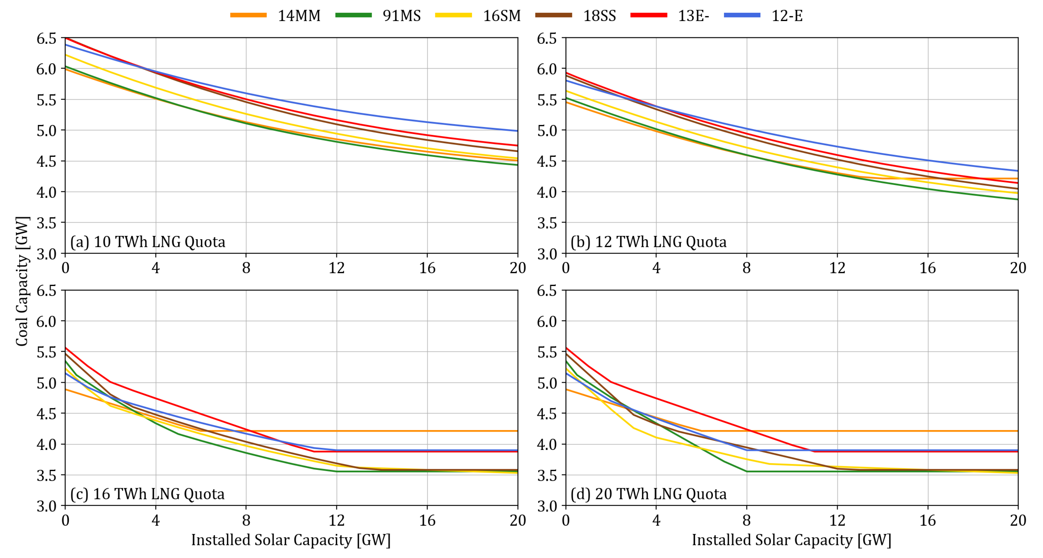
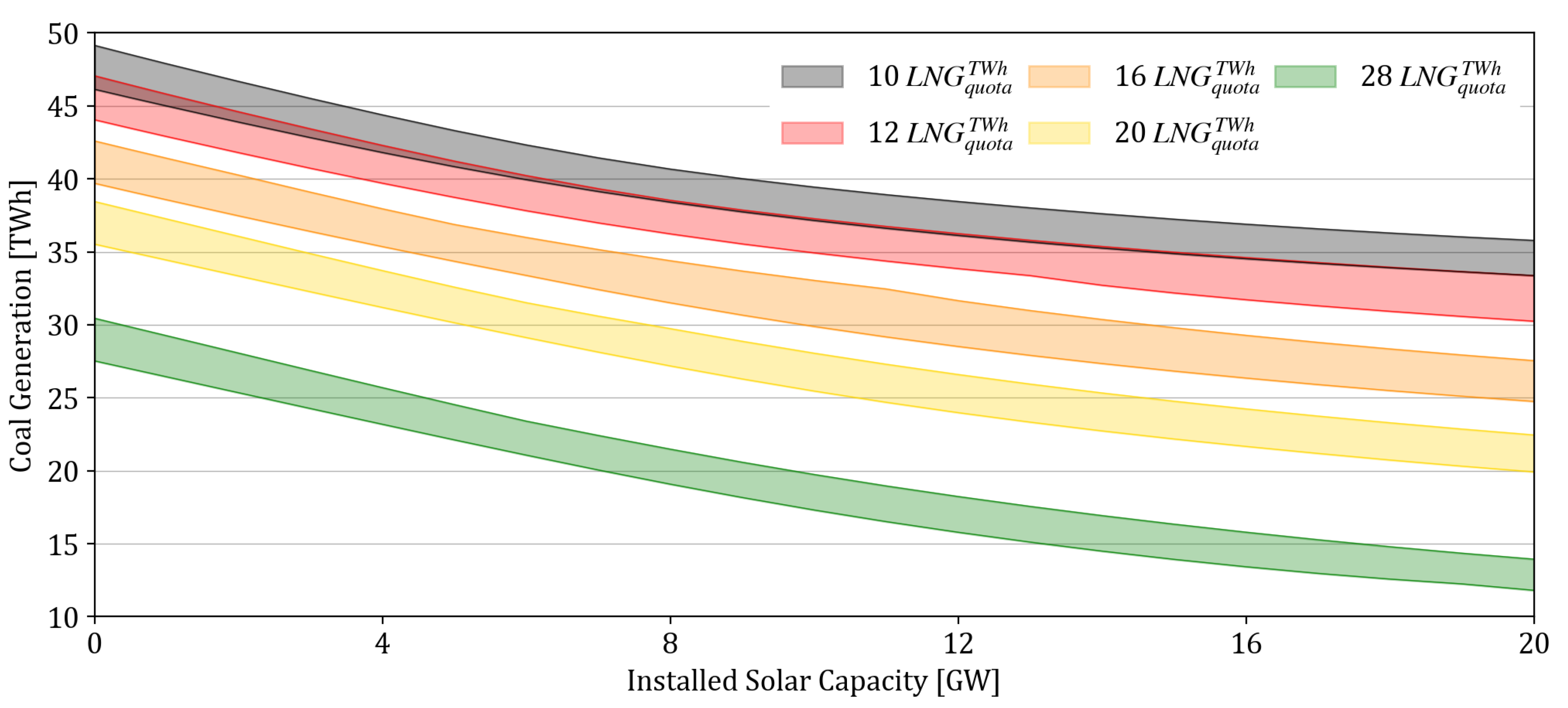
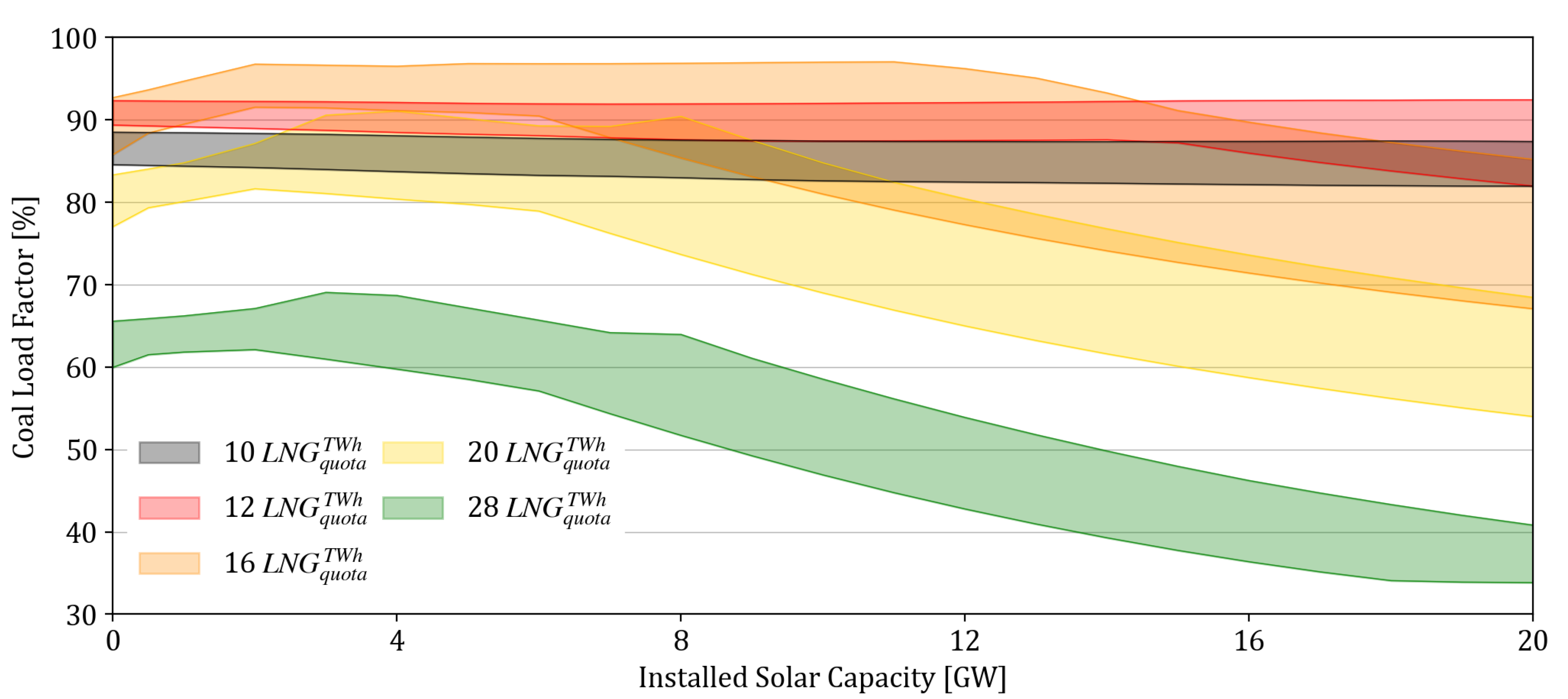
Although it cannot phase-out coal, the results show that solar energy has enough potential to be the driver for coal decommissioning with LNG’s help. It has also been shown that the decommissioning potential is robust against yearly weather-driven demand, and standby-plants could be used for the colder and warmer periods of the year. Although solar power has limitations in reducing coal capacity, it continually decreases the necessary coal generation, thereby reducing the load factor of coal plants and the corresponding CO 2 emissions.
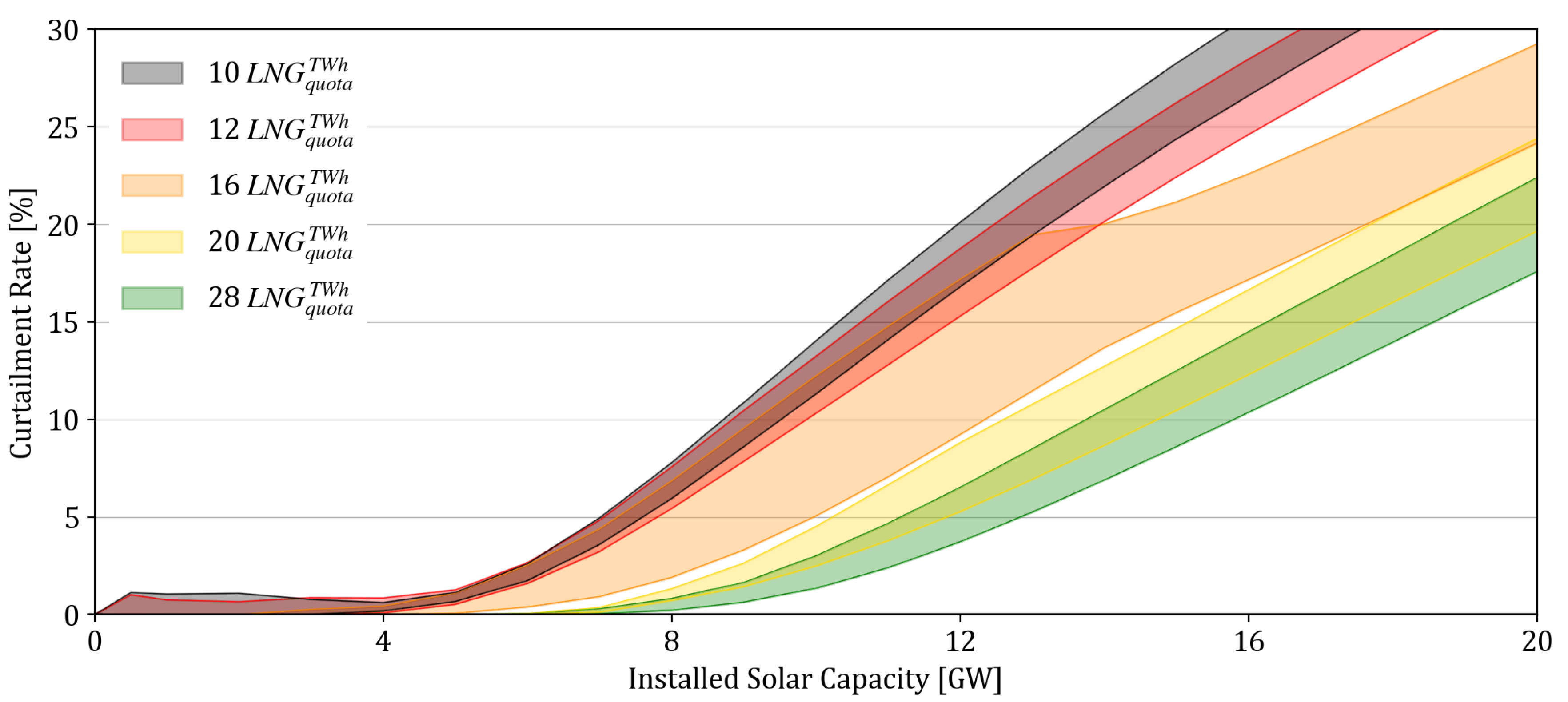
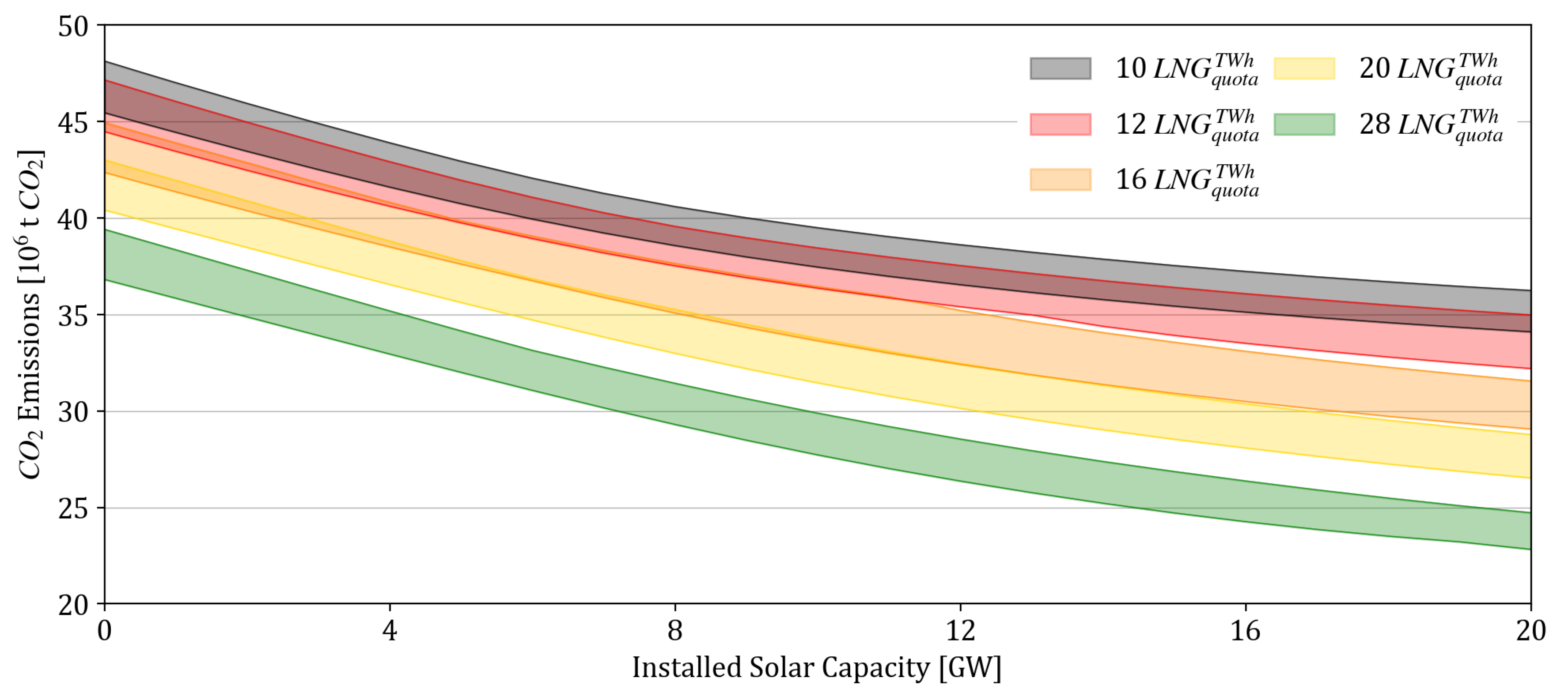
In Kyushu’s case, given the 10 GW solar capacity along with a 16 TWh complementary LNG quota, 3.5 GW of the 7 GW coal power plants could be decommissioned. This configuration is already achievable by increasing the LF of the combined-cycle plants of KyEPCO from 20% to 44%. Beyond 12 GW installed solar capacity, solar power alone has no impact on reducing the coal capacity, but it could still reduce coal generation. Compared to the reference scenario, it was shown that CO 2 emissions could be reduced by 27% through 20 GW of solar power and a 20 TWh annual LNG quota. The reduction could reach 37% if all the LNG plants in the region are utilized at 60% LF. As a related consequence, reducing coal and introducing more LNG reduced solar curtailment. This potential and limitations show that energy planners should take the necessary precautions in adding solar energy to the grid since there is an appropriate balance. Solar can reduce coal capacity, but it alone cannot phase-out coal. As was shown in Kyushu’s case, a thorough analysis of the situation that includes complementary energy sources should be considered in evaluating the potential of solar power in coal decommissioning.

4.2. Implications of Solar PV in Coal Decommissioning

Solar has its drawbacks in the form of cost and dependence on complementary flexible generators. The results show that in countries like Japan, where solar power remains to be more expensive than conventional generators—solar power presents an additional cost. Its dependence on flexible generators, which LNG currently fills, poses a threat to its ability to stand-alone. As the demand for LNG steadily increases, this will threaten its supply and price. The cost of LNG could exacerbate the cost problems of solar.
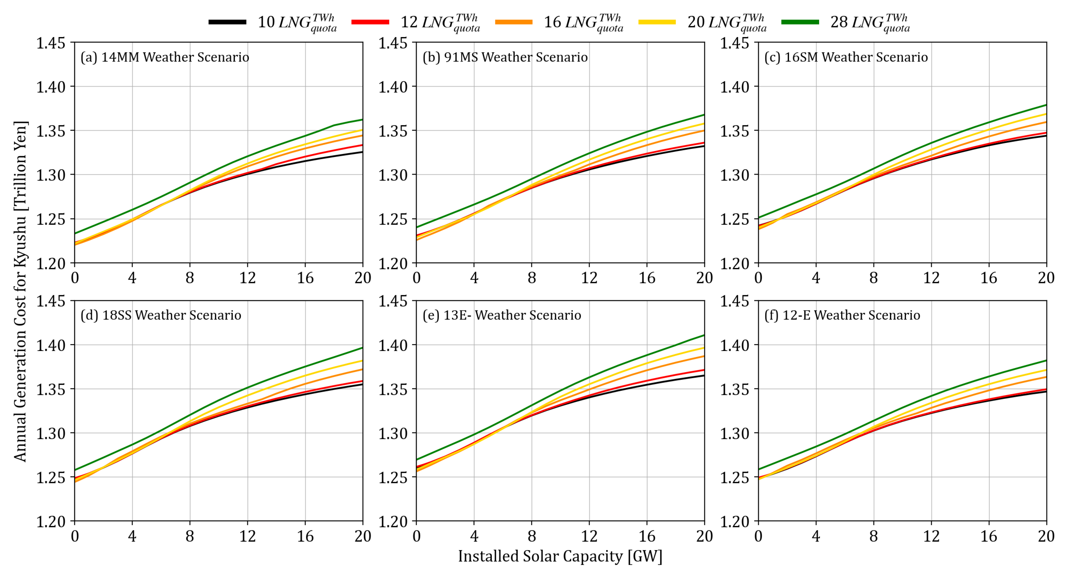
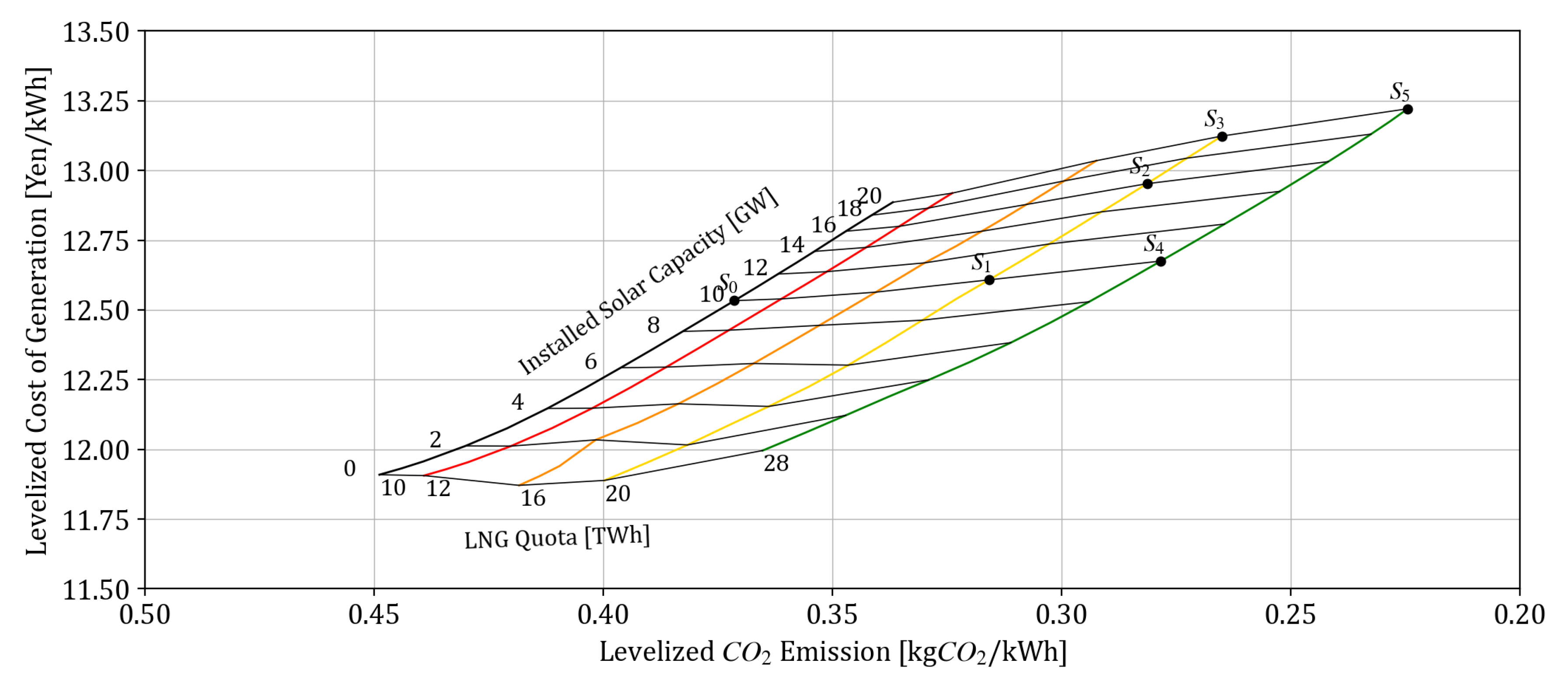
In Kyushu’s case, increasing the solar capacity from 10 GW to 16 GW and 20 GW increases the levelized cost of generation by 3.39% and 4.69%, respectively. Increasing the LNG quota has a minor impact at the moment since the current LNG price is only about 12% higher than coal. In contrast, solar is still almost twice as expensive as coal. Solar prices around the world have been decreasing, and it might decrease in Japan in the future. The impact on CO 2 and cost now becomes a policy decision, and the ratio between these two factors presents several potential combinations between LNG quota and installed solar capacity that could yield identical cost or the same CO 2 targets as seen in S 2 and S 4 . More LNG is necessary when cost is prioritized, but it will lead to more dependence on LNG. Alternatively, by investing more in solar capacity, it could lead the CO 2 reduction efforts and local power generation. This scenario entails lower dependence on both coal and LNG, which are both imported fuels. As with the previous results, the impact of weather on these values is evident, as seen in the variations in the levelized cost and levelized CO 2 emissions.

4.3. Potential Solutions beyond Solar PV

The supply and demand mismatch in winter and summer is one of the major roadblocks in the total phase-out of coal power plants through solar energy. Diurnal storage will be enough to solve the mismatch during summer, but seasonal storage or seasonal generation will be necessary for winter. Since there is still enough excess energy during peak solar production in summer, storage is the straightforward solution once these options become economically feasible. However, since there is less solar energy in winter, there is not enough excess solar energy for diurnal storage to work, which opens an opportunity for seasonal technology. Seasonal storage in the form of power-to-gas (P2G) could store the excess solar in autumn for winter. Combined heat and power (CHP) plants could be operated at a higher capacity in winter if local water heating is established.

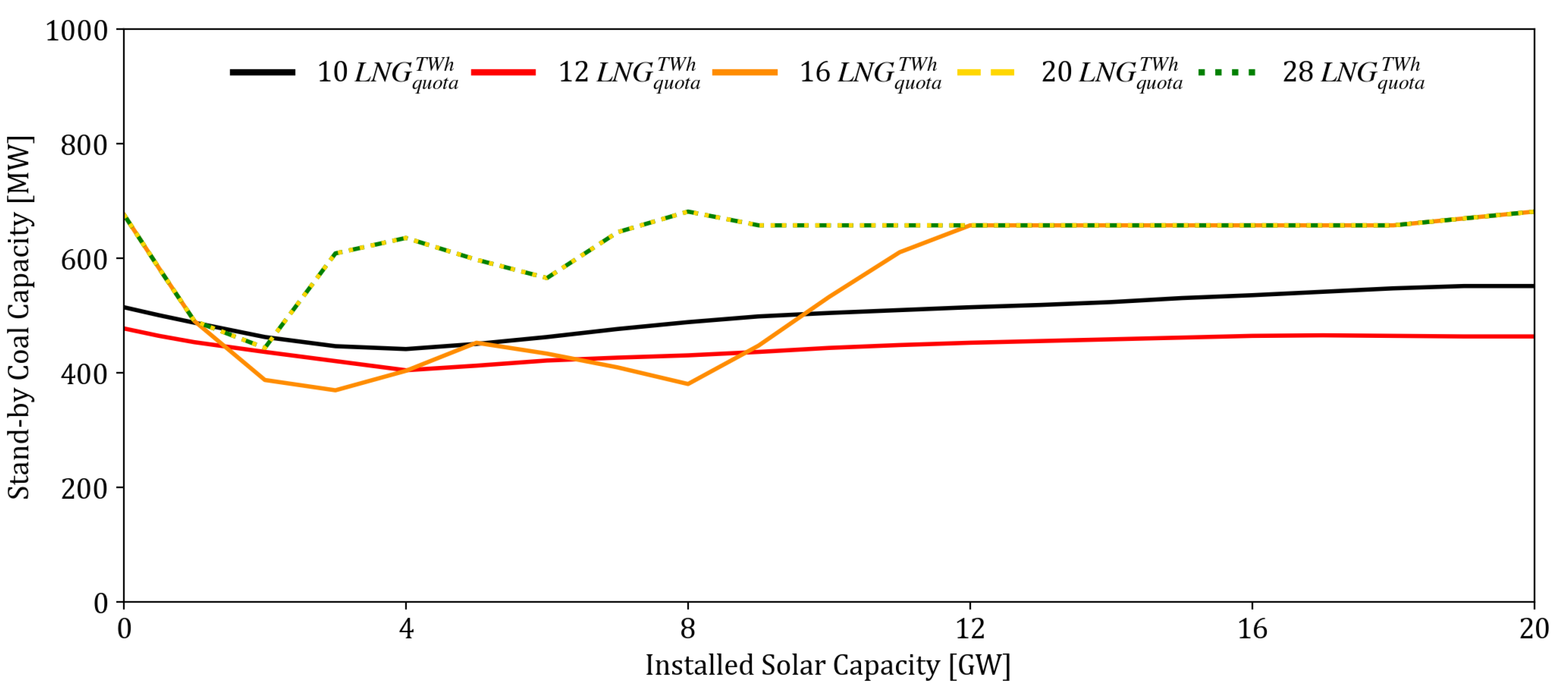
4.4. Impact of Weather on Energy Transition Plans

The stochastic nature of demand and renewable energy sources was the primary motivation for developing the weather-driven approach since energy transition recommendations should consider scenarios that will test the limits of the planned energy mix. The variations are significant at 400 MW to 600 MW coal capacity, as seen from the results. In Japan’s case, this translates to 1–3 coal power plants, but for smaller nations with smaller plants, this could be composed of more than five plants that should be on standby in the event of an extreme weather condition. Coordinating smaller plants will require more dialogue and agreements between the government and plant operators. Consequently, the government could also run standby plants to ensure the reliability of the system. It has also been shown that weather influences the potential for CO 2 reduction and the system’s overall annual generation cost. Beyond coal decommissioning, weather will remain a necessary variable in energy planning since it influences the demand, which is the primary source of stochasticity in the analysis. As more VREs are added to the green energy transition, weather becomes a crucial variable for both wind and solar. Rainfall data could also influence hydropower generation, which was not explored in this study. It could also influence the viability of PHES since this requires sufficient water reservoirs affected by rain and water evaporation. Little is known about wave energy’s potential, but the weather will also influence it since it depends on nature.

4.5. Importance and Limitation of the Proposed Approach

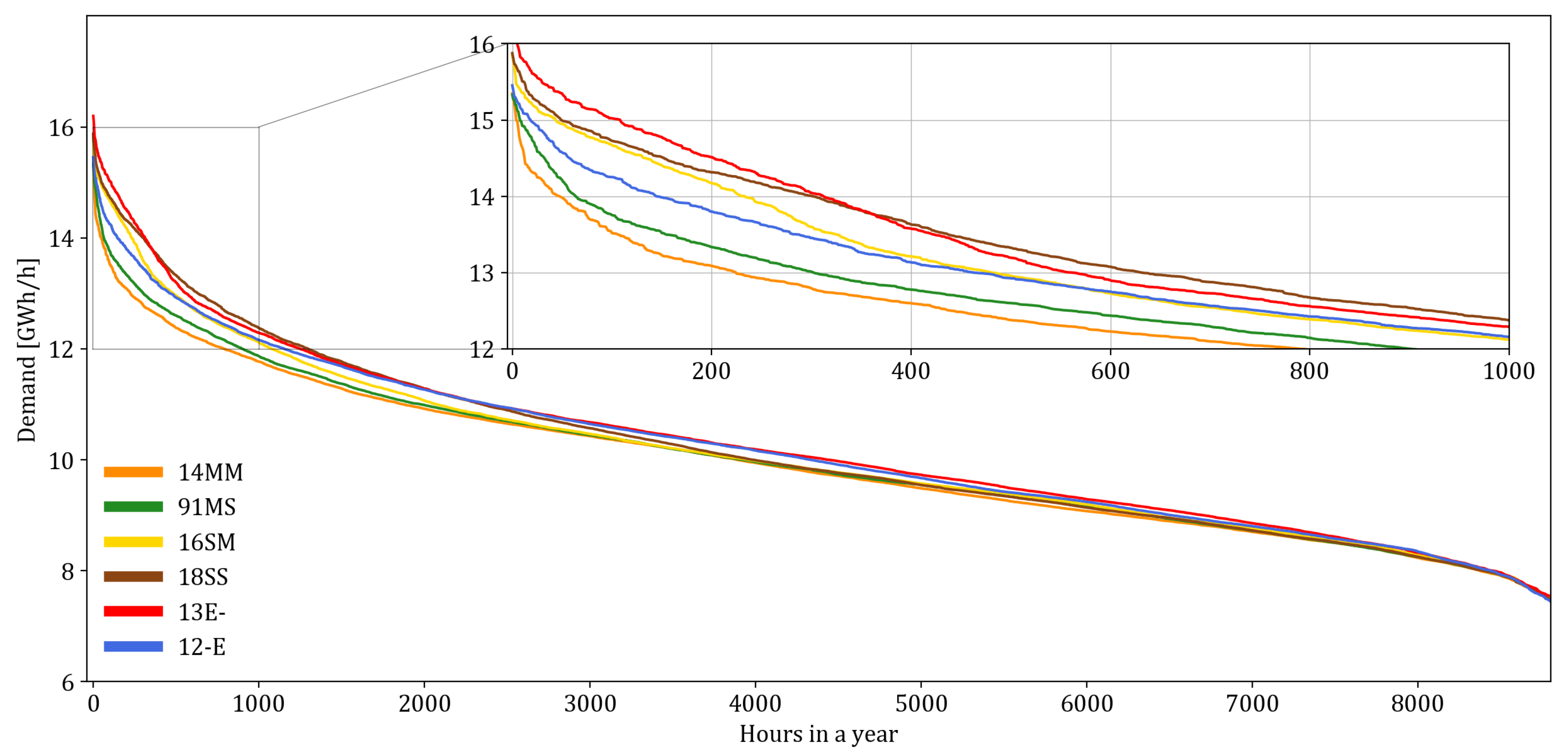
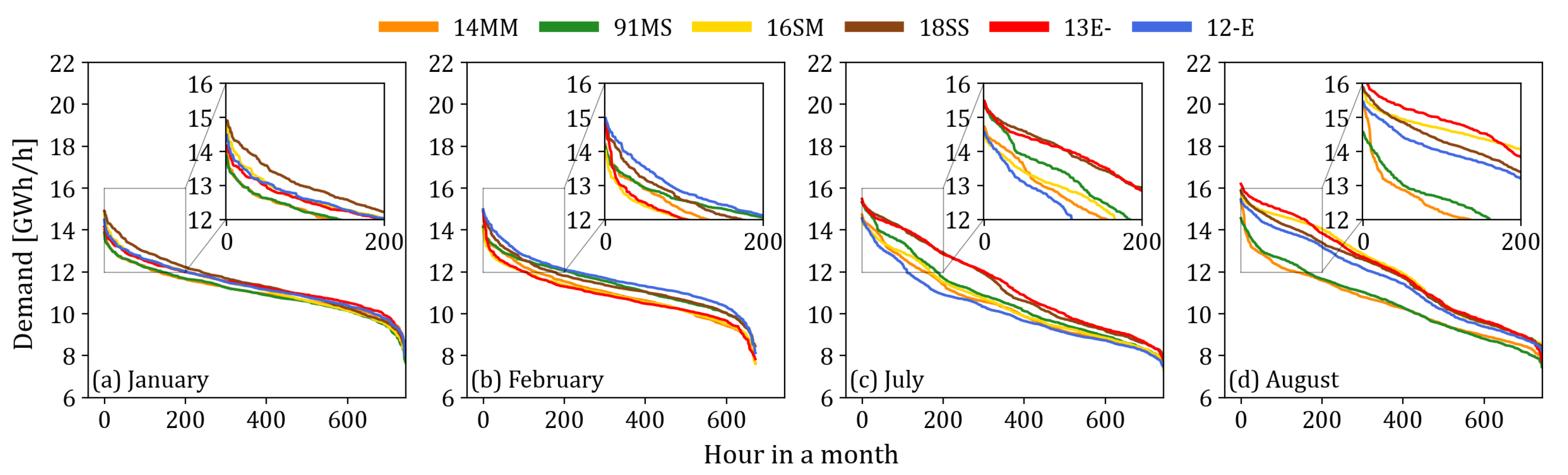
The proposed weather-driven scenario-based analysis revealed the importance of the LNG quota, demand variations, and solar generation through the annual hourly simulation. System reliability could be analyzed using the duration curve, but this does not show the hourly balance, which is greatly influenced by demand and solar generation’s stochasticity. Through careful selection of representative years, the range of potential scenarios was identified and analyzed to ensure robust results. However, the approach is dependent on the yearly assignment and is limited by the probabilistic matching of weekends and holidays to high irradiance days. The former is influenced by human behavior, while the latter is non-deterministic. Thus, although the simulation considered the yearly variations, the probability of a low irradiance day being matched to a high-demand weekday was not covered by the approach. Nonetheless, the approach can be used to provide robust recommendations for green energy transition since it covers the stochastic nature of demand and variable renewable energy. In this study, the approach was used to determine the minimum coal capacity that can ensure the system’s reliability, but it could also be used for energy storage assessments and capacity planning. This study only used a single-bus network, but it could be expanded to a national grid level by representing each region as a bus. The approach can then be used for grid expansion planning.

5. Conclusions

Driven by the idea of transitioning to a green electricity grid, an hourly power flow analysis was conducted to understand the potential, limitations, and implications of using solar energy as a driver for decommissioning coal power plants. The weather-driven scenario analysis ensured the robustness of the results and recommendations. The analysis revealed that solar power could reduce about half of Kyushu’s coal capacity with the aid of LNG. Beyond 12 GW, solar power could not reduce the minimum coal capacity necessary to ensure the system’s reliability, but it could still reduce the coal generation and the overall CO 2 emissions. The reduction in coal capacity comes at a cost, since solar power is still relatively more expensive in Japan. By installing 20 GW of solar PV systems and having 28 TWh of available LNG, the levelized CO 2 emissions could be reduced by 37%, but this would increase the levelized cost of generation by 5.6%. Most of the price increase is owed to the price of solar electricity generation, which remains high in Japan. In Kyushu’s case, this change could be achieved without constructing additional power plants, since the LNG plants are operated at a low LF. However, additional planning is necessary to acquire more LNG. Countries that use LNG plants as peak-load generators share the same potential, and the results show that a minor change in the system could have a significant impact on emission goals.
The results emphasized that solar power with the aid of LNG could partially replace coal capacity, but it alone could not phase-out coal. For energy planners who are only starting to increase their solar capacity, insights from this work could help with understanding the interactions between coal, solar, and LNG electricity generation. For planners in countries with a considerable amount of solar power (>8%), the results from this study could serve as a precaution by highlighting the risks of further increasing the solar power penetration. Although solar power helped solve midday peak power, the problem remains because it simply shifted to periods where there is no solar energy. Summer and winter are challenging periods due to the increase in peak demand. Although it is counterintuitive, solar energy is not enough during summer, or, to be more precise, misaligned since the problem occurs in the late afternoon. Diurnal storage can address the misalignment in summer, but winter presents a more intricate problem, since the solar energy is insufficient. Thus, exploring other technologies that could further complement solar energy is necessary.
The weather-driven approach revealed the importance of weather in the analysis, as it affected the results to varying degrees. In addition, 400–600 MW of standby coal capacity is necessary due to the yearly fluctuations. Coal generation, coal load factor, curtailment rate, and CO 2 emissions vary by 7–18%, 8–27%, 0–5%, and 6–8%, respectively. Identifying the representative year is crucial since it should cover the worst case, best case, and the cases in between. Energy planners and policymakers should consider the weather when analyzing energy plans, as it could provide a range of values that can guide them in making the correct decisions. Since the approach can generate scenarios based on weather data, it could also be used for storage assessment and capacity planning. The approach could also be used for grid expansion planning by increasing the number of buses and modeling multiple demands. These energy planning topics could also benefit from the range of insights generated through the weather-driven approach.

Author Contributions

Conceptualization, S.M.G.D. and K.N.I.; methodology, S.M.G.D.; software, S.M.G.D.; validation, S.M.G.D. and K.N.I.; formal analysis, S.M.G.D.; investigation, S.M.G.D.; resources, K.N.I.; data curation, S.M.G.D.; writing—original draft preparation, S.M.G.D.; writing—review and editing, K.N.I.; visualization, S.M.G.D.; supervision, K.N.I. All authors have read and agreed to the published version of the manuscript.

Funding

This research received no external funding.

Data Availability Statement

The data and code presented in this study are openly available on GitHub at https://github.com/smdumlao/demandfingerprint/tree/main/papers/coaldecommissioning (accessed on 16 April 2021).

Acknowledgments

The authors are grateful for the financial support from the Ministry of Education, Culture, Sports, Science, and Technology of Japan for the doctoral studies of Samuel Matthew Dumlao at Kyoto University. The authors are also grateful to the Ambitious Intelligence Dynamic Acceleration (AIDA) Program of Kyoto University for the financial support.

Conflicts of Interest

The authors declare no conflict of interest.

Abbreviations

The following abbreviations are used in this manuscript:
CCCombined Cycle
CHPCombined Heat and Power
DHIDiffuse Horizontal Irradiance
DNIDirect-Normal Irradiance
GEPGeneration Expansion Planning
GHIGlobal Horizontal Irradiance
IEAInternational Energy Agency
IPPIndependent Power Producer
JMAJapan Meteorological Agency
KyEPCOKyushu Electric Power Company
LNGLiquefied Petroleum Gas
METIMinistry of Economy, Trade, and Industry
MOFAMinistry of Foreign Affairs
P2GPower-to-Gas
PHESPump Hydro Energy Storage
PVSolar Photovoltaics
pvlibpvlib Python Library
PyPSAPython for Power System Analysis
VREVariable Renewable Energy
14MM2014 Mild Summer Mild Winter (Weather Scenario)
91MS1991 Mild Summer Severe Winter (Weather Scenario)
16SM2016 Severe Summer Mild Winter (Weather Scenario)
18SS2018 Severe Summer Severe Winter (Weather Scenario)
13E-2013 Extreme Summer (Weather Scenario)
12-E2012 Extreme Winter (Weather Scenario)
L N G q u o t a T W h LNG Availability (TWh)
S o l a r c a p G W Solar Capacity (GW)
G e n e r a t i o n t e c h k W h Annual Generation (kWh)
C o s t t e c h J P Y / k W h Cost of Electricity Generation (JPY/kWh)
E m i s s i o n t e c h k G C O 2 2 / k W h CO 2 Emission (kgCO2/kWh)

References

  1. Martinot, E. Grid Integration of Renewable Energy. Annu. Rev. Environ. Resour. 2016, 223–254. [Google Scholar] [CrossRef]
  2. REN21. Renewables 2020 Global Status Report. 2020. Available online: https://www.ren21.net/gsr-2020/ (accessed on 8 October 2020).
  3. Japan Ministry of Economy, Trade, and Industry. Japan’s Fifth Strategic Energy Plan (Provisional Translation). 2018. Available online: https://www.enecho.meti.go.jp/en/category/others/basic_plan/5th/pdf/strategic_energy_plan.pdf (accessed on 8 October 2020).
  4. Kyushu Electric Company. Supply and Demand Information (Japanese). 2019. Available online: http://www.kyuden.co.jp/wheeling_disclosure.html (accessed on 20 February 2021).
  5. International Energy Agency. Status of Power System Transformation. 2019. Available online: https://www.iea.org/reports/status-of-power-system-transformation-2019 (accessed on 6 March 2021).
  6. Deutscher Bundestag. Bundestag Passes the Coal Phase-Out Law. 2020. Available online: https://www.bundestag.de/dokumente/textarchiv/2020/kw27-de-kohleausstieg-701804 (accessed on 14 March 2021).
  7. Europe Beyond Coal. Overview: National Coal Phase-Out Announcements in Europe. 2021. Available online: https://beyond-coal.eu/wp-content/uploads/2021/01/Overview-of-national-coal-phase-out-announcements-Europe-Beyond-Coal-January-2021.pdf (accessed on 14 March 2021).
  8. Government of Canada. Coal Phase-Out: The Powering Past Coal Alliance. 2018. Available online: https://www.canada.ca/en/services/environment/weather/climatechange/canada-international-action/coal-phase-out.html (accessed on 14 March 2021).
  9. Kumar, S.; Kwon, H.T.; Choi, K.H.; Cho, J.H.; Lim, W.; Moon, I. Current status and future projections of LNG demand and supplies: A global prospective. Energy Policy 2011, 39, 4097–4104. [Google Scholar] [CrossRef]
  10. Shell Corporation. LNG Outlook 2020. 2020. Available online: https://www.shell.com/energy-and-innovation/natural-gas/liquefied-natural-gas-lng/lng-outlook-2020.html (accessed on 16 March 2021).
  11. Nikkei Asia. Severe Winter Forecast Sparks Recovery in Asia’s LNG Prices. 2020. Available online: https://asia.nikkei.com/Business/Markets/Commodities/Severe-winter-forecast-sparks-recovery-in-Asia-s-LNG-prices (accessed on 16 March 2021).
  12. Dumlao, S.M.G.; Ishihara, K.N. Reproducing solar curtailment with Fourier analysis using Japan dataset. Energy Rep. 2020, 6, 199–205. [Google Scholar] [CrossRef]
  13. Bunodiere, A.; Lee, H.S. Renewable Energy Curtailment: Prediction Using a Logic-Based Forecasting Method and Mitigation Measures in Kyushu, Japan. Energies 2020, 13, 4703. [Google Scholar] [CrossRef]
  14. Guittet, M.; Capezzali, M.; Gaudard, L.; Romerio, F.; Vuille, F.; Avellan, F. Study of the drivers and asset management of pumped-storage power plants historical and geographical perspective. Energy 2016, 111, 560–579. [Google Scholar] [CrossRef]
  15. Li, Y.; Gao, W.; Ruan, Y.; Ushifusa, Y. The performance investigation of increasing share of photovoltaic generation in the public grid with pump hydro storage dispatch system, a case study in Japan. Energy 2018, 164, 811–821. [Google Scholar] [CrossRef]
  16. Koltsaklis, N.E.; Dagoumas, A.S. State-of-the-art generation expansion planning: A review. Appl. Energy 2018, 230, 563–589. [Google Scholar] [CrossRef]
  17. Ioannou, A.; Angus, A.; Brennan, F. Risk-based methods for sustainable energy system planning: A review. Renew. Sustain. Energy Rev. 2017, 74, 602–615. [Google Scholar] [CrossRef]
  18. Santos, M.J.; Ferreira, P.; Araújo, M. A methodology to incorporate risk and uncertainty in electricity power planning. Energy 2016, 115, 1400–1411. [Google Scholar] [CrossRef] [Green Version]
  19. Schaeffer, R.; Szklo, A.S.; de Lucena, A.F.P.; Borba, B.S.M.C.; Nogueira, L.P.P.; Fleming, F.P.; Troccoli, A.; Harrison, M.; Boulahya, M.S. Energy sector vulnerability to climate change: A review. Energy 2012, 38, 1–12. [Google Scholar] [CrossRef]
  20. Bartók, B. Changes in solar energy availability for south-eastern Europe with respect to global warming. Phys. Chem. Earth Parts A/B/C 2010, 35, 63–69. [Google Scholar] [CrossRef]
  21. Cutforth, H.; Judiesch, D. Long-term changes to incoming solar energy on the Canadian Prairie. Agric. For. Meteorol. 2007, 145, 167–175. [Google Scholar] [CrossRef]
  22. Dumlao, S.M.G.; Ishihara, K.N. Supplementary Materials: Weather-Driven Scenario Analysis for Decommissioning Coal Power Plants in High PV Penetration Grid. 2021. Available online: https://github.com/smdumlao/demandfingerprint/tree/main/papers/coaldecommissioning (accessed on 16 April 2021).
  23. Japan Meteorological Agency. Past Regional Weather Data. Available online: http://www.data.jma.go.jp/risk/obsdl/index.php (accessed on 8 January 2021).
  24. Holmgren, W.F.; Hansen, C.W.; Mikofski, M.A. Pvlib python: A python package for modeling solar energy systems. J. Open Source Softw. 2018, 3, 884. [Google Scholar] [CrossRef] [Green Version]
  25. Brown, T.; Hörsch, J.; Schlachtberger, D. PyPSA: Python for Power System Analysis. J. Open Res. Softw. 2018, 6. [Google Scholar] [CrossRef] [Green Version]
  26. Knüpfer, K.; Dumlao, S.M.G.; Esteban, M.; Shibayama, T.; Ishihara, K.N. Analysis of PV Subsidy Schemes, Installed Capacity and Their Electricity Generation in Japan. Energies 2021, 14, 2128. [Google Scholar] [CrossRef]
  27. Agency for Natural Resources and Energy. Electric Power Survey Statistical Data. Available online: https://www.enecho.meti.go.jp/statistics/electric_power/ep002/results_archive.html (accessed on 8 January 2021).
  28. Holmgren, W.; Andrews, R. Pvlib: TMY to Power Tutorial. Available online: https://nbviewer.jupyter.org/github/pvlib/pvlib-python/blob/master/docs/tutorials/tmy_to_power.ipynb (accessed on 8 January 2021).
  29. Erbs, D.; Klein, S.; Duffie, J. Estimation of the diffuse radiation fraction for hourly, daily and monthly-average global radiation. Sol. Energy 1982, 28, 293–302. [Google Scholar] [CrossRef]
  30. Ministry of Land, Infrastructure, Transport and Tourism. Japan Power Plant GIS Data. 2007. Available online: https://nlftp.mlit.go.jp/ksj/jpgis/datalist/KsjTmplt-P03.html (accessed on 8 June 2020).
  31. Japan Beyond Coal. Japan Coal Plant Database. 2020. Available online: https://beyond-coal.jp/map-and-data/ (accessed on 29 September 2020).
  32. Kyushu Electric Power Company. KYUDEN Group Environmental Data Book 2020. 2020. Available online: http://www.kyuden.co.jp/var/rev0/0270/6338/env_data_2020.pdf (accessed on 18 March 2021).
  33. Ministry of Economy, Trade and Industry of Japan. Recent Situation of Thermal Power Generation. 2017. Available online: https://www.meti.go.jp/shingikai/enecho/shoene_shinene/sho_energy/karyoku_hatsuden/pdf/h29_01_04_00.pdf (accessed on 18 March 2021).
  34. Ministry of Economy, Trade and Industry of Japan. Report on Power Generation Costs. 2015. Available online: https://www.enecho.meti.go.jp/committee/council/basic_policy_subcommittee/mitoshi/cost_wg/006/pdf/006_05.pdf (accessed on 10 March 2021).
  35. Advisory Panel to the Foreign Minister on Climate Change. Promote New Diplomacy on Energy through Leading Global Efforts against Climate Change. 2018. Available online: https://www.mofa.go.jp/files/000337158.pdf (accessed on 10 March 2021).
  36. Ministry of Environment of Japan. Evaluation of CO2 Emissions of Thermal Power Generation. 2016. Available online: https://www.env.go.jp/council/06earth/y0613-16/ref06-16.pdf (accessed on 10 March 2020).
Figure 1. The proposed weather-driven scenario-based analysis approach capable of handling weather-related variations in electricity demand and solar energy production.
Energies 14 02389 g001
Figure 2. Temperature deviation of the representative year from the comfortable temperature of 18 °C to 22 °C.
Energies 14 02389 g002
Figure 3. Generating the demand fingerprint based on the demand and temperature data.
Energies 14 02389 g003
Figure 4. The weekly demand clusters of Kyushu from FY2016–2019.
Energies 14 02389 g004
Figure 5. Correlation of Temperature and Demand in Kyushu.
Energies 14 02389 g005
Figure 6. Temperature-dependent demand generation.
Energies 14 02389 g006
Figure 7. Sample demand synthesis for 2018.
Energies 14 02389 g007
Figure 8. Configuration of the single-bus network used in the optimization.
Energies 14 02389 g008
Figure 9. Duration curve of the synthetic demand.
Energies 14 02389 g009
Figure 10. Monthly duration curve of the synthetic demand.
Energies 14 02389 g010
Figure 11. Minimum required coal capacity as installed solar capacity increases, and various LNG quotas.
Energies 14 02389 g011
Figure 12. Standby coal capacity needed to ensure that the electricity grid can still handle weather-driven demand variations.
Energies 14 02389 g012
Figure 13. The coal generation in different LNG quota scenarios.
Energies 14 02389 g013
Figure 14. The coal load factor in different LNG quota scenarios.
Energies 14 02389 g014
Figure 15. Projected curtailment rates assuming the optimal coal capacity was followed, with the corresponding annual LNG quotas.
Energies 14 02389 g015
Figure 16. Range of CO 2 emissions for various scenarios in Kyushu.
Energies 14 02389 g016
Figure 17. Annual generation costs for various scenarios in Kyushu.
Energies 14 02389 g017
Figure 18. Levelized generation cost and CO 2 emissions for the warmer year (16SM) scenario. The CO 2 emissions (abscissa) are formatted in decreasing order to emphasize the trend. S 0 reflects the current situation, and S 1 S 5 are the potential future scenarios.
Energies 14 02389 g018
Table 1. Weather stations in Kyushu.
PrefecturePrefecture No.Precinct CodeBlock Code
Fukuoka408247,807
Saga418547,813
Nagasaki428447,817
Kumamoto438647,819
Oita448347,815
Miyazaki458747,830
Kagoshima468847,827
Table 2. Share of solar power installations (%) in the prefectures.
Prefecture20122013201420152016201720182019
Fukuoka34.8324.9825.1625.1424.6223.8623.0622.26
Saga8.488.047.226.966.986.786.856.50
Nagasaki8.989.679.119.8210.029.669.469.48
Kumamoto15.8713.3114.5214.2614.5014.4614.7514.63
Oita11.4015.0713.2613.0812.5412.0012.5112.34
Miyazaki8.6611.5911.9411.7811.6612.5312.8213.03
Kagoshima11.7717.3418.7918.9619.6820.7220.5521.76
Table 3. Average monthly demand share (%) in Kyushu from 2016 to 2019.
PrefectureJANFEBMARAPRMAYJUNJULAUGSEPOCTNOVDEC
Fukuoka38.2538.2838.1337.6637.3237.2637.4737.6037.2136.8537.2037.79
Saga7.837.998.108.028.028.208.127.797.867.908.047.94
Nagasaki9.559.519.359.429.409.259.289.609.489.239.229.39
Kumamoto13.7613.8213.7313.4213.3713.6413.7813.8313.9113.8113.7213.76
Oita10.6110.6410.7210.9711.1810.9210.5810.2710.3810.8110.9310.94
Miyazaki8.498.278.458.758.778.728.638.548.548.818.738.55
Kagoshima11.5011.4911.5211.7711.9412.0012.1312.3712.6212.6012.1611.63
Table 4. Representative years of different weather scenarios in Kyushu.
SummerWinterRepresentativeLegendFrequency *Comment
MildMild201414MM2Low variability
MildSevere199191MS6Colder year
SevereMild201616SM8Warmer year
SevereSevere201818SS5High variability
Extreme-201313E-5Extreme Summer
-Extreme201212-E4Extreme Winter
* Occurrence in the past 30 years from 1990 to 2019.
Table 5. Generators in Kyushu as of FY2019.
GeneratorPower (MW)Carrier Output min (%)Ramp Limit (%)
Coal7037Coal301
LNG5250Gas1540
Geothermal160Renewable1000
Biomass450Renewable1000
Solar9000Renewable0100
Nuclear4140Non-GHG1000
Wind355Renewable1540
Hydro4000Renewable1540
Table 6. LNG quota scenarios.
LNG Power Plant LNG quota 1 TWh LNG quota 2 TWh LNG quota 3 TWh LNG quota 4 TWh LNG quota 5 TWh
CategoryCapLFGenLFGenLFGenLFGenLFGen
KyEPCO Steam1800203.15203.15203.15203.15609.46
KyEPCO CC2825204.95276.684410.896014.856215.34
IPP625402.19402.19402.19402.19603.29
Total5250 10.29 12.03 16.23 20.19 28.09
Capacity (Cap) in MW; load factor (LF) in %; generation (Gen) in TWh.
Table 7. Cost of electricity generation (JPY/kWh).
TechnologyMETI 2014METI 2030MOFA 2018 *Applied **
Nuclear10.110.1-10.1
Coal12.312.9612.3
LNG13.713.41013.7
Wind21.913.910–22 (15)17.9
Geothermal19.219.2-19.2
Hydro11.011.0-11.0
Biomass12.613.3-12.6
Solar (Comm)24.312.78–36 (17)18.5
Solar (Home)29.412.5--
* Values in parentheses are the average values; ** used in the calculation; as of April 2021: 100 JPY = 0.92 USD = 0.77 EUR.
Table 8. Monthly solar power generation load factor (%) using the irradiance of the representative years.
YearJANFEBMARAPRMAYJUNJULAUGSEPOCTNOVDEC
201413.2811.4714.8914.5917.039.9411.459.0511.3813.8011.6110.15
199112.0912.4411.8912.4911.148.7311.1813.3312.4012.2814.6210.41
20167.9412.4015.3411.8413.5910.6713.7515.9010.529.1812.6411.93
201811.5513.9515.6916.9913.4512.2614.0015.3310.0714.1914.609.19
201311.0313.7714.8416.3416.099.5314.7014.7014.7313.2912.0110.67
201211.029.5613.3117.0114.538.8410.3012.1512.1015.2011.117.20
Mean11.1512.2714.3314.8814.319.9912.5613.4111.8712.9912.779.93
Table 9. Cost and CO 2 emissions of the reference scenario.
14MM91MS16SM18SS13E-12-EMean
Levelized Cost (JPY/kWh)12.546412.526612.533112.581912.582012.516012.5477
Levelized CO 2 (kgCO 2 /kWh)0.36400.36830.37140.36790.37230.37640.3700
As of April 2021: 100 JPY = 0.92 USD = 0.77 EUR.
Table 10. Cost increase from the reference scenario.
ScenariosIncrease in Cost per kWh (%)
NoName Solar cap GW LNG quota TWh 14MM91MS16SM18SS13E-12-EMean
S 1 Increase L N G q u o t a T W h 110200.560.530.600.740.750.590.63
S 2 Increase S o l a r c a p G W 116203.343.383.353.463.613.173.39
S 3 Increase S o l a r c a p G W 220204.614.754.714.754.934.404.69
S 4 Increase L N G q u o t a T W h 210281.201.071.131.341.281.141.19
S 5 Increase both20285.515.525.495.866.005.225.60
Table 11. CO 2 emission decrease from the reference scenario.
ScenariosDecrease in CO 2 Emission per kWh (%)
NoName Solar cap GW LNG quota TWh 14MM91MS16SM18SS13E-12-EMean
S 1 Increase L N G q u o t a T W h 11020−13.50−12.74−12.55−12.91−12.94−12.18−12.80
S 2 Increase S o l a r c a p G W 11620−22.78−22.53−22.10−22.66−22.78−21.02−22.31
S 3 Increase S o l a r c a p G W 22020−27.05−27.18−26.62−27.24−27.29−25.15−26.75
S 4 Increase L N G q u o t a T W h 21028−23.77−23.24−22.93−23.37−23.09−22.27−23.11
S 5 Increase both2028−36.45−38.32−37.84−37.97−37.58−35.70−37.31
Publisher’s Note: MDPI stays neutral with regard to jurisdictional claims in published maps and institutional affiliations.

