Article

Investigating the Converter-Driven Stability of an Offshore HVDC System

1
Institute of High Voltage Equipment and Grids, Digitalization and Energy Economics, RWTH Aachen University, Templergraben 55, 52062 Aachen, Germany
2
DNV, Arnhem Utrechtseweg 310, 6812 AR Arnhem, The Netherlands
*
Author to whom correspondence should be addressed.
Energies 2021, 14(8), 2341; https://doi.org/10.3390/en14082341
Submission received: 23 February 2021 / Revised: 1 April 2021 / Accepted: 18 April 2021 / Published: 20 April 2021
(This article belongs to the Special Issue Hybrid AC/DC Grid)

Abstract

:
Offshore wind farms are increasingly built in the North Sea and the number of HVDC systems transmitting the wind power to shore increases as well. To connect offshore wind farms to adjacent AC transmission systems, onshore and offshore modular multilevel converters transform the transmitted power from AC to DC and vice versa. Additionally, modern wind farms mainly use wind turbines connected to the offshore point of common coupling via voltage source converters. However, converters and their control systems can cause unwanted interactions, referred to as converter-driven stability problems. The resulting instabilities can be predicted by applying an impedance-based analysis in the frequency domain. Considering that the converter models and system data are often confidential and cannot be exchanged in real systems, this paper proposes an enhanced impedance measurement method suitable for black-box applications to investigate the interactions. A frequency response analysis identifies coupling currents depending on the control system. The currents are subsequently added to the impedance models to achieve higher accuracy. The proposed method is applied to assess an offshore HVDC system’s converter-driven stability, using impedance measurements of laboratory converters and a wind turbine converter controller replica. The results show that the onshore modular multilevel converter interacts with AC grids of moderate short-circuit ratios. However, no interactions are identified between the offshore converter and the connected wind farm.

1. Introduction

With the increasing number of High-Voltage Direct Current (HVDC) links integrated into the Alternating Current (AC) transmission system and converters, power electronics relying on complex control systems play a more dominant role in system stability. In particular, remote offshore wind farms are connected by high-voltage cables and rely on HVDC technology due to the high reactive power demand of AC-based systems. Additionally, modern wind farms utilize mainly fully-scaled Voltage Source Converters (VSCs) for the offshore grid connection. VSC and state-of-the-art HVDC converters, such as Modular Multilevel Converters (MMCs), have response times that are significantly faster compared to traditional power system components [1]. Several interactions of converters with the connected AC system or other converters have been reported. For instance, in 2014, the offshore wind farm Bard Offshore 1 had to be shut down due to high oscillations in the grid current and voltage at frequencies other than the grid frequency of 50 Hz [2]. In addition, the 2015-commissioned HVDC INELFE system connecting Spain and France experienced resonances between the HVDC system and the AC grid [3,4]. Furthermore, unexpected oscillations were observed in a weak part of the China Southern Grid’s transmission system after a Static Synchronous Compensator (STATCOM) was put into operation [5].
Consequently, electromagnetic phenomena need to be considered for assessing the stability of modern power systems. Hence, the classical power system stability classification was extended to consider the impact of power electronic interfaced technologies [6]. Whereas this interaction phenomenon is often referred to in the literature as harmonic stability [7,8], the updated stability definition classifies the aforementioned interaction incidents as converter-driven stability with fast interactions [6]. Converter-driven instabilities are mainly caused by the converters’ control system that interacts with the AC grid impedance [6,9]. However, disclosing manufacturer-specific converter control systems is highly improbable due to intellectual property concerns [10], making it challenging to model the converters’ real frequency behavior. In addition, Transmission System Operators (TSOs) are unlikely to share details of their grid models with other parties.
Several methods and approaches exist to investigate converter-driven stability. For example, eigenvalue analyses have the advantage that they can assess stability globally for an entire system. Additionally, participation factors provide additional information about controllers and parameters affecting system stability [11]. However, this requires a state-space model of the entire system, including linearized component models. Therefore, state-space modeling is not applicable when detailed information of the components is not provided. A promising method to investigate converter-driven stability problems is the Impedance-based Stability Criterion (IbSC) that models a system as two subsystems with frequency-dependent impedances and uses classical control theory to assess the stability in the frequency domain [12,13]. The IbSC allows for a direct and straightforward stability assessment. By providing Phase Margins (PMs), it indicates how close a system is to instability [7,14]. It can also be consecutively applied to assess the stability of large-scale systems by defining different interfaces and subsystems [15]. Moreover, due to short computation times, numerous scenarios can be investigated, which would not be possible when using Electromagnetic Transient (EMT) simulations [7,14]. The IbSC requires frequency-dependent impedance models of the system components, which can be derived analytically using small-signal linearization techniques [16,17,18] or numerically on the basis of EMT simulations or measurements using frequency sweep techniques [19,20].
In the literature, stability analyses often utilize analytical impedance models derived based on a white-box approach that implies that the converter structure and the control system’s block diagrams are known [14,21,22,23]. This approach offers excellent insight into the cause of interactions and can be used to investigate the impact of specific controllers and parameters on stability [24]. However, it does not allow for stability analyses of black-boxed systems and is not applicable for industrial applications. Moreover, analytical models are often based on a simplified electrical structure of converters so that the real frequency behavior of components might not be considered [11,25,26]. In addition, the models often neglect control loops, assuming that they are not relevant [16]. To deal with the three-phase nature of the transmission system, authors advocate modeling the impedances in the dq-domain [27,28]. Couplings between phases and frequencies are included in the models using a 2 × 2 impedance matrix. The authors demonstrate that neglecting the coupling can result in false stability predictions [28,29]. However, approaches that rely on impedance representations in the dq-domain require the definition of a common reference angle θ for the dq-domain transformation [30,31,32]. Thus, this approach makes it challenging to use different entities’ impedance models (e.g., converter manufacturer and TSO). They would have to align their models on a reference angle which is not applicable for industrial studies.
As a result, utilized approaches are not aimed at investigating real and industrial systems. They cannot be applied to black-boxed systems such as converter controller replicas, representing the frequency behavior of industrial control systems. Thus, this paper presents an approach to assess the stability of a system, where no detailed information of a converter control system is provided and where the system’s models (e.g., converter and grid impedance) are provided by different entities. The approach builds upon a frequency-sweep approach to assess the converter-driven stability [33,34]. Not requiring full-system knowledge, this approach makes it possible to employ impedance models of a black-boxed system such as a converter controller replica or measurement-based models of physical laboratory converters. Additionally, models can be provided by different entities for the stability assessment. For instance, a converter manufacturer can provide the impedance model to a TSO. The TSO is then able to investigate the converter-driven stability using their grid impedance model. In this paper, the proposed impedance derivation method in [33,34] is extended to include additional coupling currents resulting from the frequency sweep measurements. To determine these additional coupling currents, the spectrum of physical MMC is analyzed using a laboratory system—here referred to as the MMC Test Bench (TB). The derived MMC impedances are used to investigate the stability of an MMC in grid-following control mode and the adjacent AC system, representing the onshore side of an HVDC link. The AC grid impedance is calculated analytically with respect to different Short-Circuit Ratios (SCRs). On the offshore side, the stability of a wind farm and the offshore MMC operating in grid-forming control mode is investigated utilizing the impedance measurement of an offshore Wind Turbine (WT) VSC controller replica. Therefore, this paper contributes to the evaluation of converter-driven stability under realistic conditions by evaluating the stability of an offshore HVDC system, employing laboratory converters and converter control replica systems for the analysis.
The paper is structured as follows: First, the IbSC is presented, and an overview of the impedance derivation approach is given. The IbSC is validated by comparing the stability predictions to the results of an EMT time-domain simulation. Subsequently, Section 3 demonstrates the extended frequency-sweep approach and shows how the additional measurements are incorporated in the impedance models. Section 4 presents the Control Hardware in the Loop (CHiL) TB setup for the WT VSC controller replica impedance measurement. Based on the derived impedance models, the following stability analysis in Section 5 presents and discusses the results of the onshore and offshore test case. Concluding the paper, the main findings are given in Section 6.

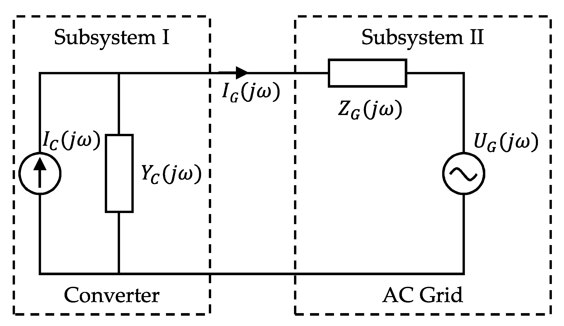
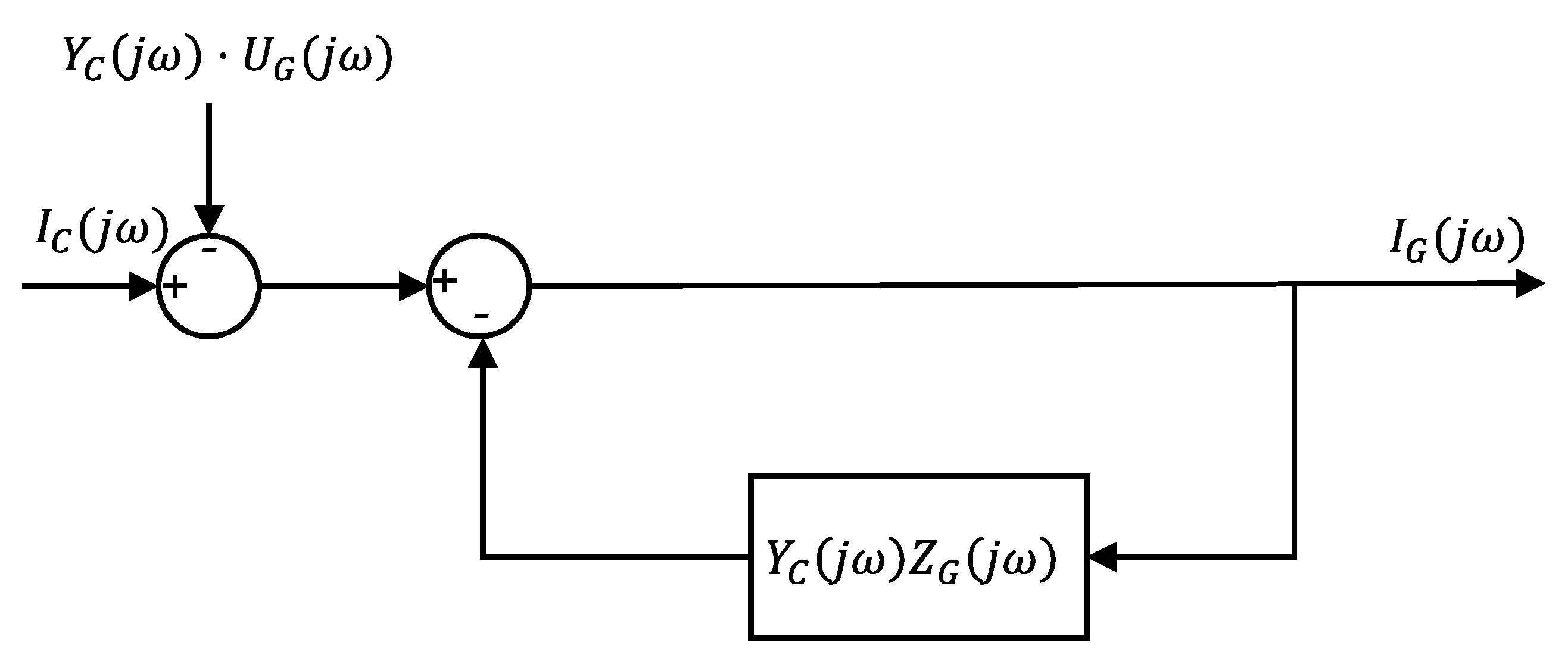
2. Impedance-Based Stability Assessment

2.1. Impedance-Based Stability Criterion

Initially developed for the design of input filters of converters [12,35], the IbSC is a widely used method to assess converter-driven stability in the frequency domain. Because this method avoids time-consuming EMT simulations, it facilitates the analysis of numerous test cases [7,14]. Assuming that a system can be divided into two separate subsystems, the stability can be assessed by classical control theory tools, such as the Nyquist criterion or Bode plots analyzing the loop gain of the system. Figure 1 shows the equivalent circuit diagram of a system divided into two subsystems representing a converter and an AC grid, aiming to assess interactions between the subsystems’ impedances.
The frequency behavior of the subsystems is modeled by the respective admittance Y C ( j ω ) and impedance Z G ( j ω ) with ω = 2 π . Deriving the current to
I G ( j ω ) = I C ( j ω ) 1 1 + Y C ( j ω ) Z G ( j ω ) U g ( j ω ) Y C ( j ω ) 1 + Y C ( j ω ) Z G ( j ω ) ,
which can be rearranged to
I G ( j ω ) = [ I C ( j ω ) U g ( j ω ) · Y C ( j ω ) ] · 1 1 + Y C ( j ω ) · Z G ( j ω )
shows that the system resembles that of a negative feedback loop system, as shown in Figure 2.
As a result, the feedback loop gain Y C ( j ω ) Z G ( j ω ) can be evaluated by the simplified Nyquist criterion to determine the stability of the overall system. Assuming an open-loop stable system that does not contain any right-half plane poles, the system’s stability can be graphically assessed. This assumption implies that both subsystems’ impedances and admittances need to be individually stable. This means that the subsystem with the admittance Y C is stable if it can operate in ideal grid conditions (infinite short-circuit power) and that the subsystem with the impedance Z G is stable in no-load conditions [13]. These conditions are typically fulfilled, since a converter should be able to operate stably in ideal conditions, and the AC grid should be stable when not connected to the converter. In addition to the Nyquist plot, a Bode plot analysis offers a more intuitive stability assessment. By calculating the phase difference of Y C ( j ω ) and Z G ( j ω ) at the magnitude intersection frequencies, the PM can be determined showing how close the system is to instability. However, considering only the PM for stability assessments can lead to false stability predictions in certain situations when the slope of the impedance phase is not evaluated [36]. As a result, additional magnitude and phase conditions should be considered [36] if the results are not verified by additional Nyquist plots.

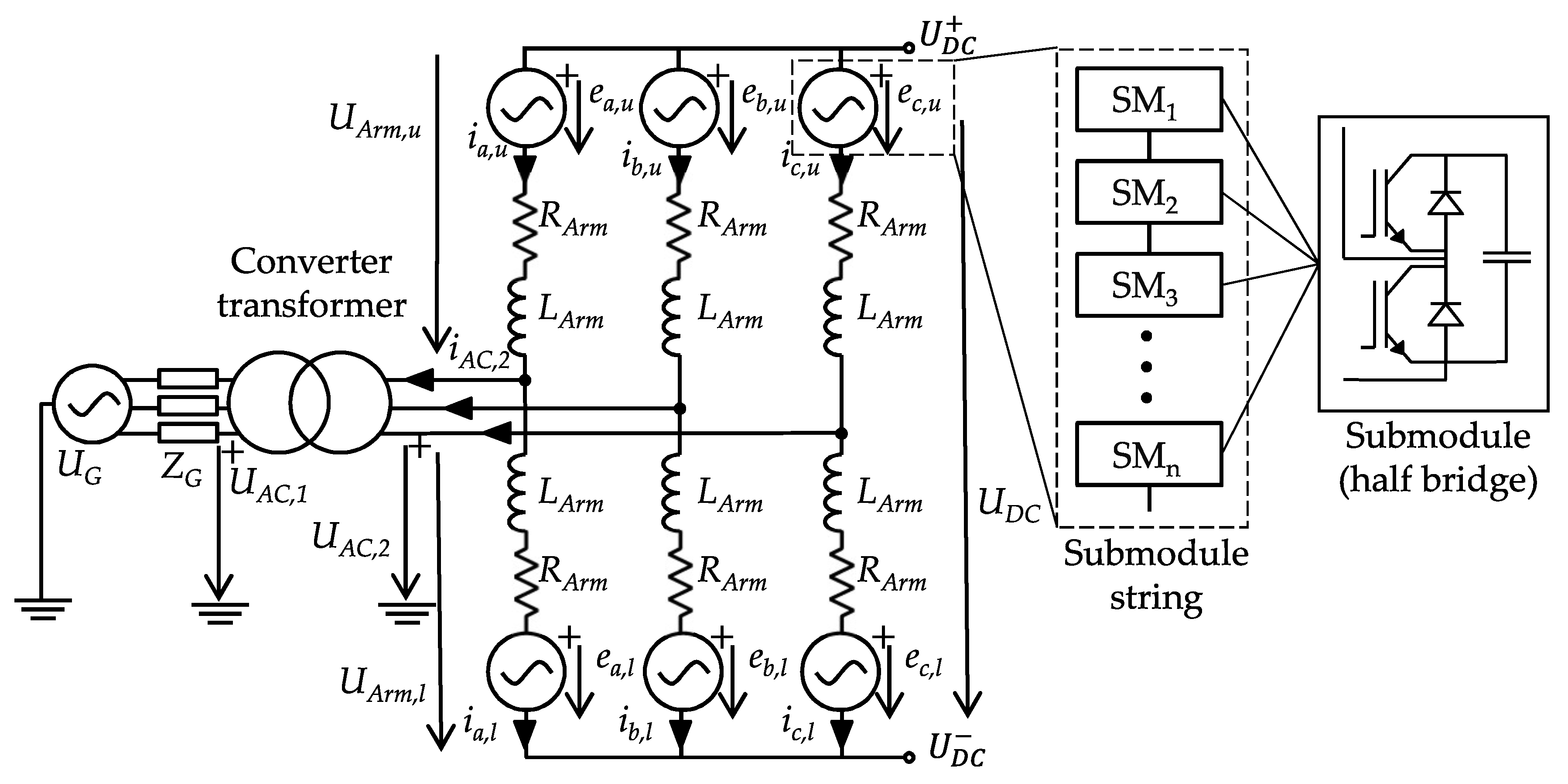
2.2. Impedance Model Derivation

Using the IbSC to assess converter-driven stability requires the derivation of impedance models that represent the frequency behavior of the investigated components and systems. Impedance models are typically derived in the dq-domain [7,29] or in positive and negative sequence [37,38]. As pointed out in Section 1, dq-domain impedances require the definition of a reference angle for the dq-transformation. This means that both subsystems’ impedances have to be aligned on a common angle, typically the grid voltage angle, θ . This contradicts the objective of this work, that the impedance models can be derived independently and exchanged between two different parties without prior harmonization [31]. However, sequence-domain impedance models do not inherently consider couplings between frequencies [28]. Thus, in this work, impedances are derived in the sequence domain that allows for separate positive- and negative-sequence impedance models [37]. To determine the impact of couplings, the frequency spectrum is evaluated for potential coupling frequencies that affect the impedances [39].
Impedance models of active components such as MMC can be derived analytically by deriving transfer functions based on the electrical model and the block diagrams of the converter control system [22,24,26]. While this approach offers insight into the causes and dependencies of different controllers and parameters on the system stability, it requires full knowledge of the converter and its control system. Therefore, analytically-derived impedances cannot be derived when investigating the frequency behavior of black-boxed manufacturer converters such as converter controller replica systems. Thus, a numerical impedance derivation method is developed in [33] and applied to laboratory MMC in [34]. The method can be applied without having access to the control system of the converters. Figure 3 gives an overview of the developed method. The user can define the Measurement Parameters (MPs), M P p e r t , and M P f , that parameterize a measurement series.
The method is separated into the test circuit and the part processing the input and output signals. A Device Under Test (DUT), such as the MMC, is connected to a grid circuit that sets the required operating points for the DUT by providing a grid voltage or current. When deriving the converter impedance, the grid impedance is set to virtually zero so that it does not influence the measurements. The grid impedance is calculated independently using an analytical formula as in (3). Additionally, it can also be measured on the basis of an EMT time-domain model. Figure 4 shows the circuit diagram for deriving the MMCs’ impedances. While measuring the impedance of MMC 1, MMC 2 ensures a stable operation on the Direct Current (DC) side by controlling either the DC voltage or the power flow [34]. Depending on the operation mode, the perturbation source consecutively injects additional small-signal voltages or currents at a frequency f p e r t . The frequency generator provides the frequency series and additional MPs defined by the user. Prior experiments have shown that a magnitude of 5 of the grid voltage or current is a good trade-off for having a perturbation signal that is large enough to be measured but also small enough to not disturb the operation of the converter. The DUT is subjected first to a positive- and then negative-sequence voltage or current in two separate measurement series. The measured voltage U m e a s ( t ) and current I m e a s ( t ) are simultaneously evaluated for the frequencies f e v a l ( t ) by the signal processor to determine the magnitudes | U ( f ( t ) ) | and | I ( f ( t ) ) | and the phase angles U ( f ( t ) ) and I ( f ( t ) ) at f = f e v a l . The evaluated frequencies comprise the applied perturbation frequency f p e r t . Nonetheless, additional frequencies can also be evaluated. The impedance calculator then applies a sequence transformation on the frequency-domain signals. When the system is perturbed in positive sequence, the positive-sequence components of the signals determine the positive-sequence impedance. Likewise, the negative sequence signals determine the negative-sequence impedance for the negative-sequence perturbation. The impedance | Z ( f ( t ) ) | Z ( f ( t ) ) is determined online during the measurements and is therefore time-dependent [33]. The final frequency-dependent impedance | Z D U T ( f ) | Z D U T ( f ) is calculated by taking the average of each time period in which a single perturbation frequency is applied. For this work, the frequency-sweep developed in [33,34] is enhanced by implementing the frequency generator and signal processor on a Field Programmable Gate Array (FPGA), facilitating a time step in the nanosecond range.
In the case of high-voltage components, a more complex test circuit needs to be used. For this purpose, a Power Hardware in the Loop (PHiL) test-setup has been built to measure the impedances of converters in the range of several M W . Additional step-up transformers connect a converter with the 10.5 k V medium voltage grid and a 1.32 M W DC supply directly feeds the DC-link of the DUT [40,41]. For the M W test circuit, a current source perturbation is preferable because a voltage perturbation source would need to absorb all of the current which is injected by the DUT into the test circuit. Thus, a perturbation current is always applied by the power amplifier. However, it is challenging to achieve a sufficiently high bandwidth for a MW-level test circuit, because the power amplifier bandwidth is typically inversely proportional to its rating [41].

2.3. Validation

The impedance-based stability analysis and the impedance derivation method are validated by deriving the impedance of a simulated EMT time-domain MMC model. The stability is assessed for different AC grid impedances with varying short-circuit power S S C , G . Simulating the same system and scenarios in the time-domain verifies the frequency-domain results. Figure 5 shows the system used for the validation. The parameters of the simulated MMC model are given in Table 1.
On the DC side of the MMC, the voltage is held constant to U D C . The simulated MMC model is based on a Type 5 Average Value model, consisting of controlled voltage sources that represent the Submodule (SM) string of each arm [42]. The MMC control system is a cascaded vector control and is designed as an energy-based control, where the energy control loops of the MMC are explicitly implemented [43]. A high-level overview of the control system is given in Figure 6.
The upper-level controls are responsible for controlling the reference values of the dispatch control, provided by the converter operator. When operating in grid-following control mode, the MMC can control the active and reactive power and the DC and AC voltage. Additional current controllers and the Phase-Locked Loop (PLL) synchronize the converter with the AC grid. In grid-forming control mode, the converter directly defines the grid voltage magnitude, frequency, and angle. An oscillator at fixed angular frequency generates the grid frequency instead of the PLL. The upper-level controls then provide the reference arm voltage e A C * and e D C * to the lower-level controls, particularly, the converter control, which ensures a dynamic, but also stable, operation of the converter. For this purpose, the horizontal and vertical balancing controls that the average energy stored in the MMC and the SM is symmetrically distributed among the MMC arms, ensuring an equal, average AC and DC power output. The circulating current control suppresses undesired currents flowing within the converter due to voltage imbalances of the converter arms. Finally, the submodule control determines the semiconductors’ switching states according to the provided reference voltage e * u , l using Pulse-Width Modulation (PWM) or Nearest-Level Modulation (NLM) as potential modulation techniques. The capacitor balancing determines which SM are switched so that the energy of the capacitors is evenly distributed.
The AC grid is modeled as a Thevenin equivalent voltage source U G with the grid impedance
Z G = R G + j 2 π f G L G .
Its parameters are given in Table 2 and depend on the SCR that is defined according to the short-circuit power S S C , G and the converter power P n , M M C with
S C R = S S C , G P n , M M C .
Typically, the SCR is considerate high for S C R 5 , moderate for 3 < S C R < 5 , low for S C R 3 , and very low for S C R 2 [44]. When the MMC’s impedance is derived, an additional perturbation voltage source is added between the grid impedance Z G and the converter transformer.

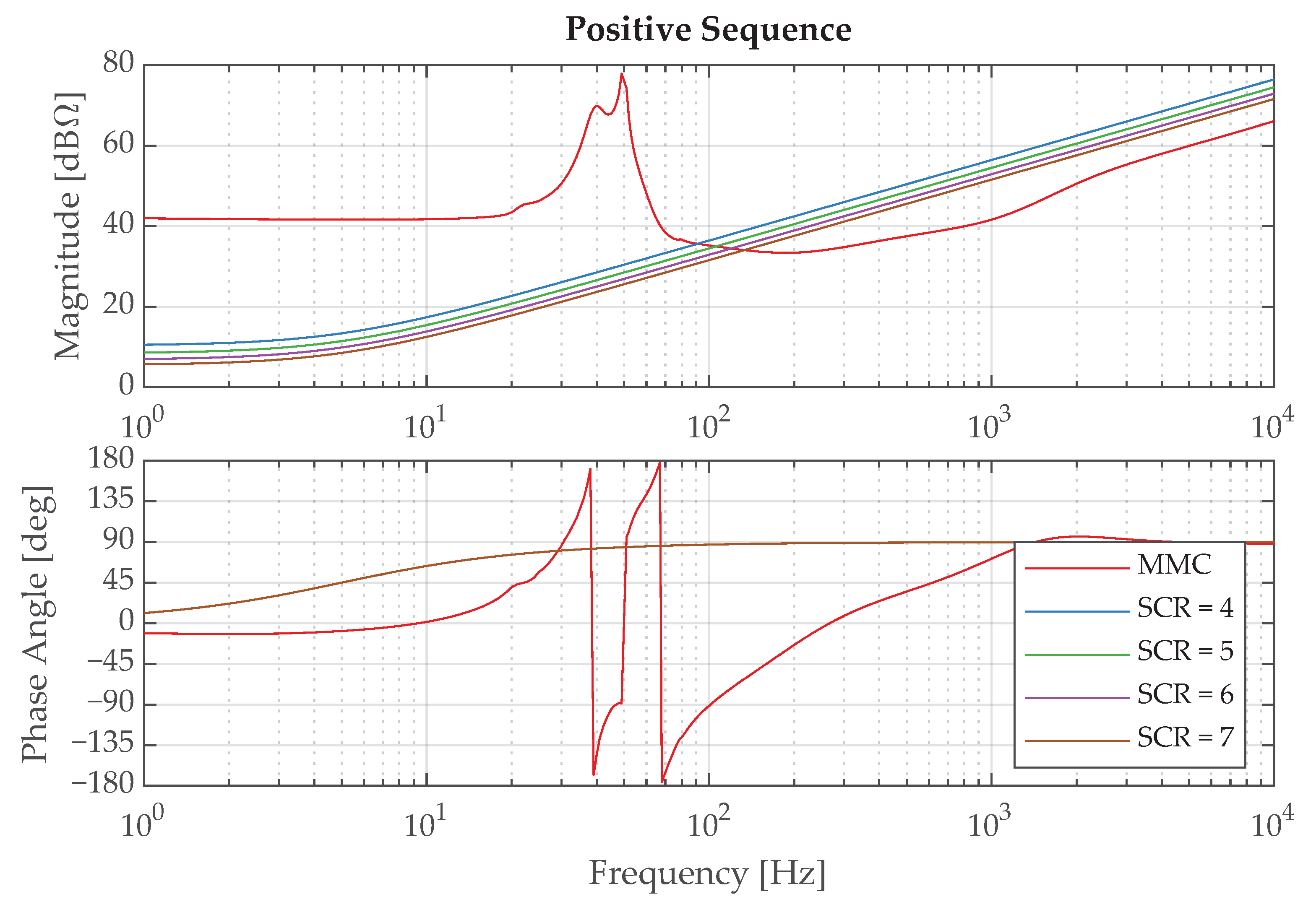
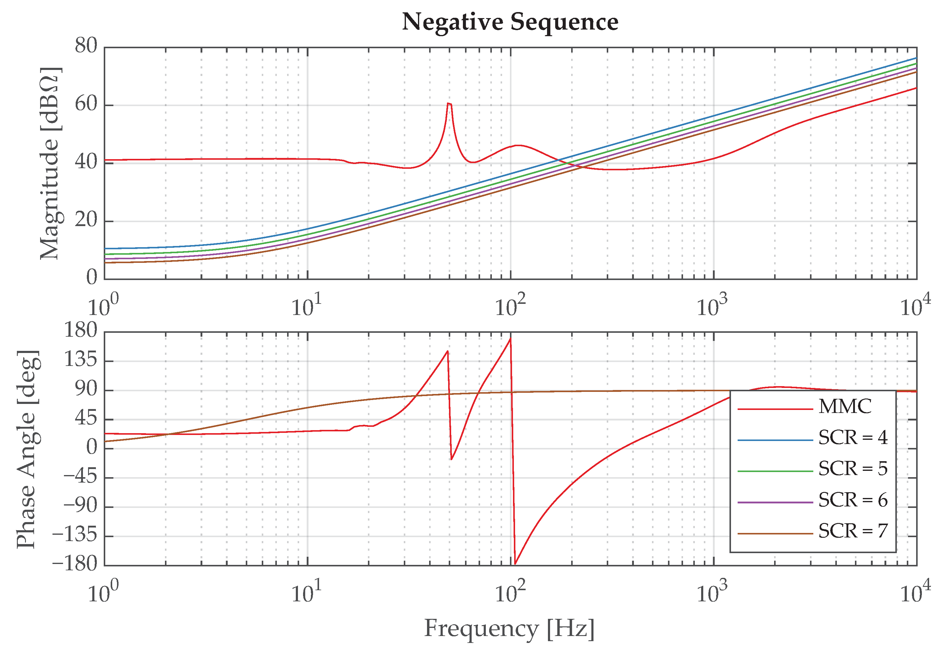
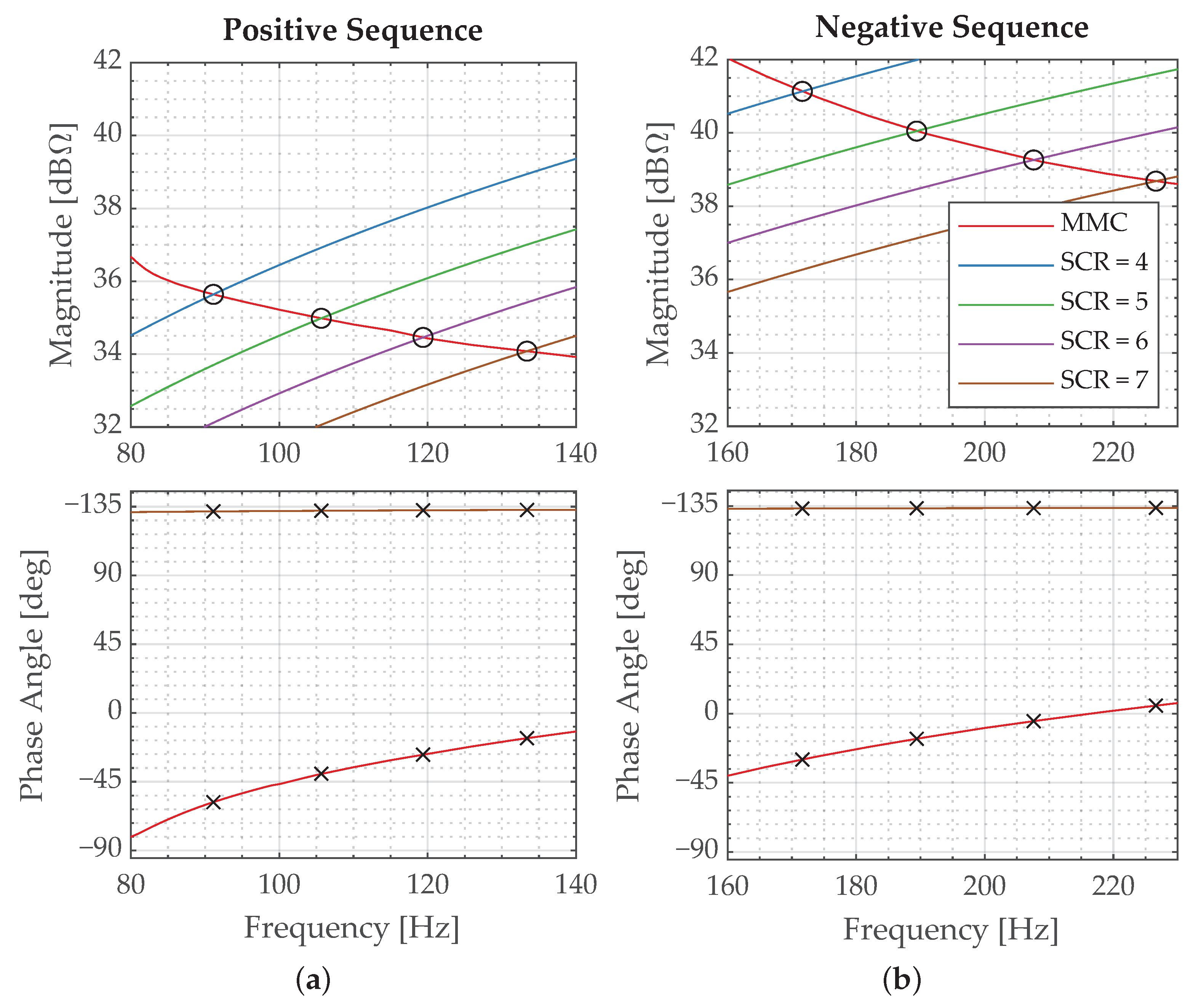
2.3.1. Frequency-Domain Stability Assessment

The converter-driven stability of the AC grid and the simulated MMC model circuit is assessed by the IbSC. Being in grid-following control mode, the MMC controls the grid current and can be represented by a current source with parallel admittance. Hence, the MMC impedance Z M M C ( j ω ) represents the converter admittance Y C ( j ω ) in the equivalent circuit diagram shown in Figure 1. Consequently, the corresponding loop gain can be derived as in Figure 2 and yields Z G ( j ω ) Z M M C ( j ω ) . For simplicity, hereinafter, the argument of the variables is indicated by the frequency only, while still referring to a complex variable. The PMs of the system are then derived at the intersection frequencies f P M where
Z G ( f P M ) = Z M M C ( f P M ) .
Subtracting the phase angle difference at f P M from 180 makes it possible to graphically determine the PMs of the Bode plot with
P M = 180 arg Z G ( f P M ) Z M M C ( f P M ) = 180 arg Z G ( f P M ) Z G ( f P M ) .
To assess the system’s overall stability, both positive- and negative-sequence systems need to be considered [37]. If either the positive-sequence or the negative-sequence system analysis determines an unstable system, the overall system is considered to be unstable. If both positive- and negative-sequence systems are stable, then also the overall system is concluded to be stable. Therefore, Figure 7 and Figure 8 depict the Bode plots for positive- and negative-sequence impedances. They show that the magnitude of the MMC intersects those of the AC grid at frequencies close to 100 Hz and 200 Hz , respectively. Furthermore, the plots reveal that with decreasing SCR, the intersection frequencies decrease also. For lower frequencies, the differences of the phase angle increase, potentially reaching 180 and leading to a negative PM.
Figure 9 show a close-up of the Bode plots around the intersection frequencies for the different SCRs. Marking the magnitudes and phase angles at f P M , they reveal that for a S C R = 4 , the phase difference exceeds 180° for the positive-sequence impedance. The PMs given in Table 3 show that for a S C R = 4 and f P M , p o s = 91 Hz , the PM is negative indicating that the system becomes unstable when the SCR is decreased from 5 to 4. Because the the PM provides only a sufficient stability condition [36], the results of the Bode plot analysis are verified by additional Nyquist plots presented in Figure A1 in the Appendix A, showing a clock-wise encirclement of the ( 1 , j 0 ) point for S C R = 4 and the positive-sequence impedance.

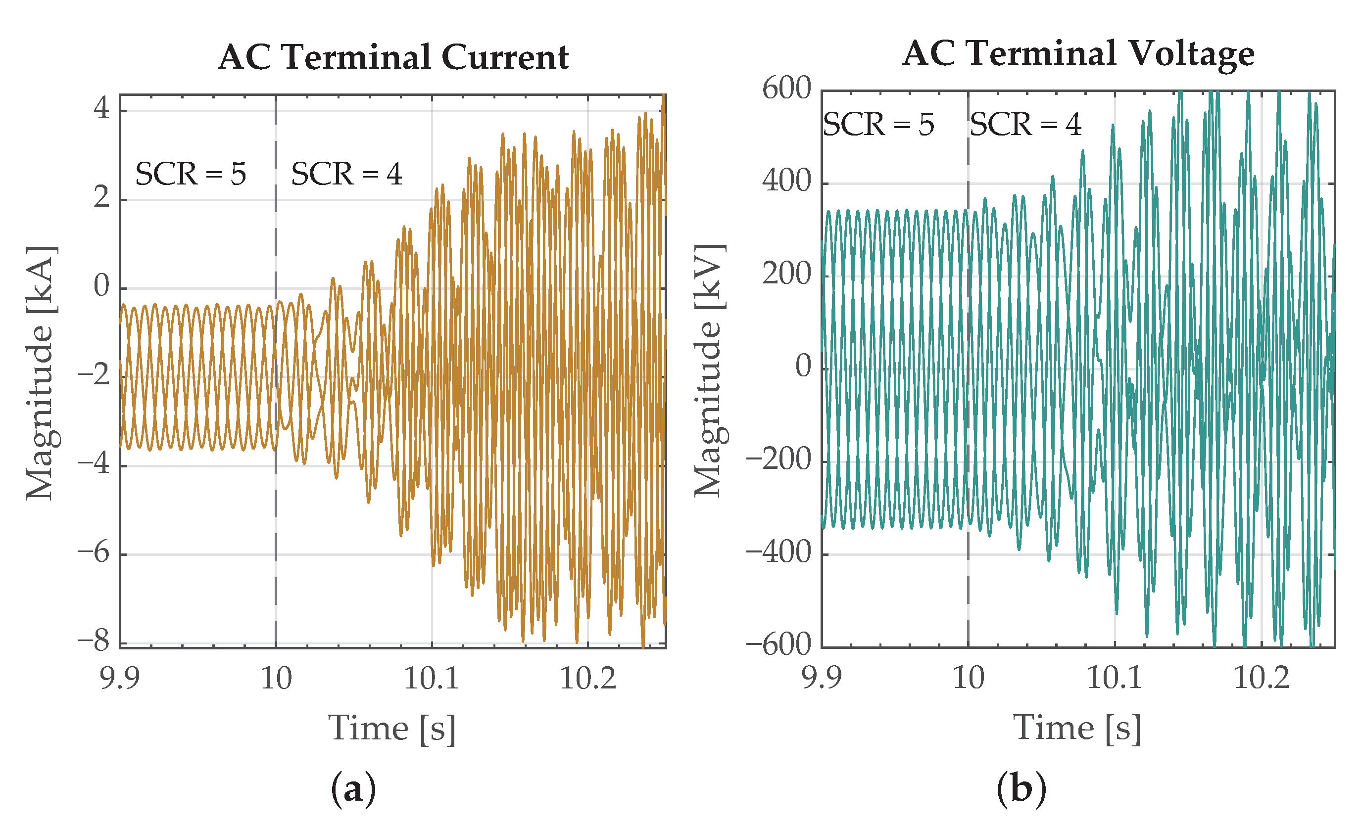
2.3.2. Time-Domain Validation

Because the frequency-domain stability assessment uses linearized impedance models, the results are verified by time-domain simulations of the same system in Matlab/Simulink. Thus, the MMC model is connected to AC grids with varying SCRs. To ensure an initial stable operation point, the MMC is initially started when connected to a strong AC grid. Figure 10 shows the current at the MMC AC terminal. After t = 4 s , the MMC is switched to an AC grid impedance with S C R = 7 Every two seconds, the AC grid impedance is reduced by an SCR value of 1. As predicted in the frequency-domain analysis, the system remains stable for AC grid impedances with an S C R = 7 to 5 . The current and voltages in Figure 11 show that high oscillations occur and an unstable operation point is reached when switching to an AC grid with S C R = 4 . Figure 12 shows the frequency spectrum of the AC terminal current and voltage after switching. Showing oscillations with a frequency of 94.5 Hz , the spectrum agrees with the previously predicted instability at f = 91 Hz . Thus, the results demonstrate that the IbSC is able to to accurately assess the converter-driven stability of a system using numerically derived impedance models.

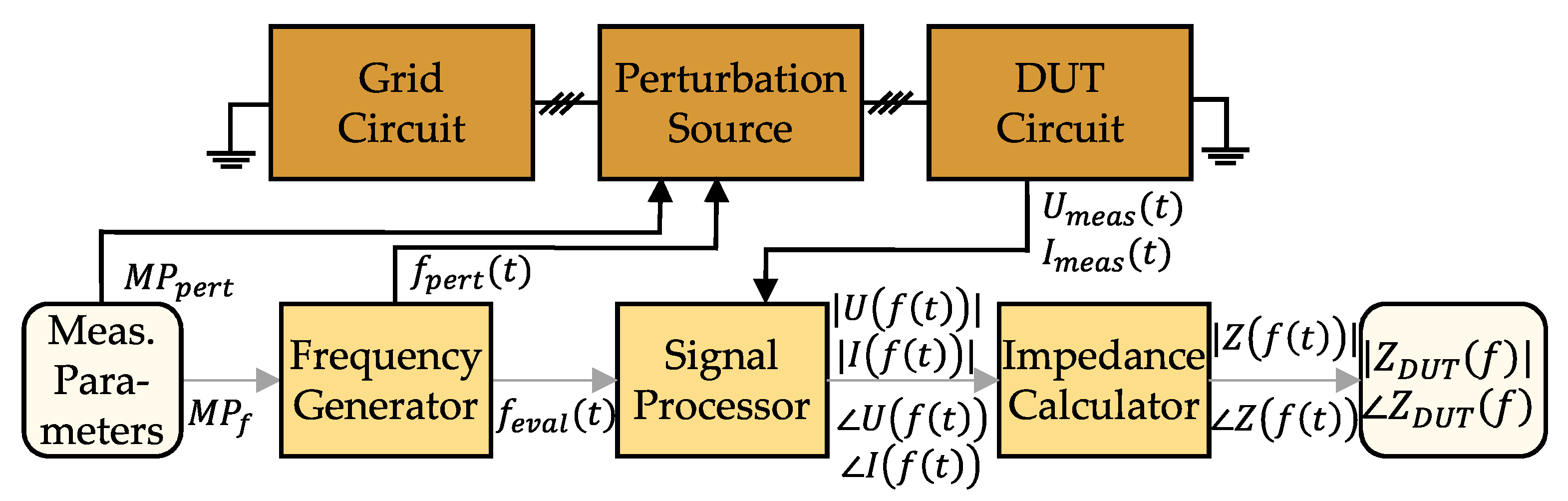
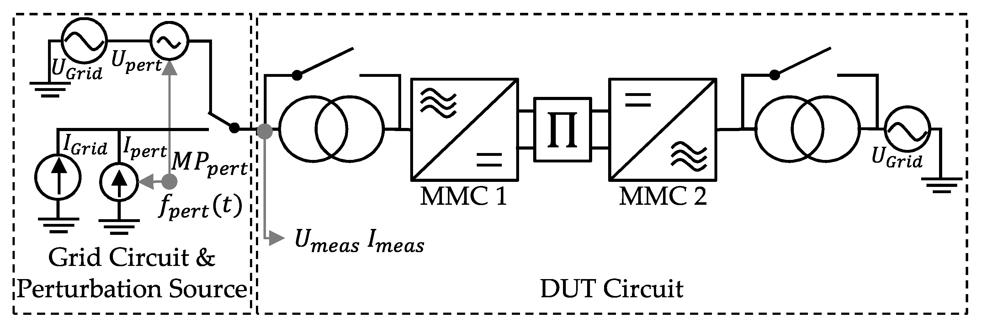
3. Extended MMC Impedance Derivation Method

Representing the frequency behavior of the MMCs, in this work, the corresponding impedance models are derived based on physical laboratory converters using the MMC TB laboratory at RWTH Aachen University. Thus, inaccuracies due to model simplifications can be avoided, and the impedance derivation method is demonstrated in a laboratory environment. First, the frequency spectrum of the MMC TB response is evaluated when being subjected to different perturbation signals to determine relevant frequency components. The MMC TB laboratory consists of several real-time simulators and low-voltage MMC with the parameters given in Table 4 [45]. For measuring the MMC impedances, two MMCs are physically connected through Pi-sections on the DC side and coupled with real-time simulators through power amplifiers on the AC side [34]. The control system is identical to the controls of the simulated MMC model as presented in Figure 6. Figure 13 illustrates the MMC TB setup that is used for deriving the laboratory MMC’s impedances. The power amplifier can be operated either in current or voltage mode. In current mode, the power amplifier connected to MMC 1 feeds in a current consisting of the grid and the perturbation current. In voltage mode, the power amplifier supplies a voltage consisting of the grid voltage superimposed by the perturbation voltage. In both cases, power amplifier 2 supplies the grid voltage for MMC 2. A detailed overview of the measurement setup can be found in [34].
The MMC TB impedance | Z T B | e φ T B is scaled up according to the scaling factors | k | and k φ [34] to align with the AC grid impedance and the 1 M W wind turbine VSC. The scaled MMC TB impedance is
Z T B , s c a l e d = | k | · | Z T B | e φ T B k φ
with
| k | = r F S 2 + ( ω · l F S ) 2 r T B 2 + ( ω · l T B ) 2
and
k φ = arctan r F S ω · l F S arctan r T B ω · l T B .
The equivalent resistance r F S and inductance l F S are calculated using the simulated full-scale MMC parameters given in Table 1, while r T B and l T B are based on the MMC TB parameters given in Table 4 as described in [34].

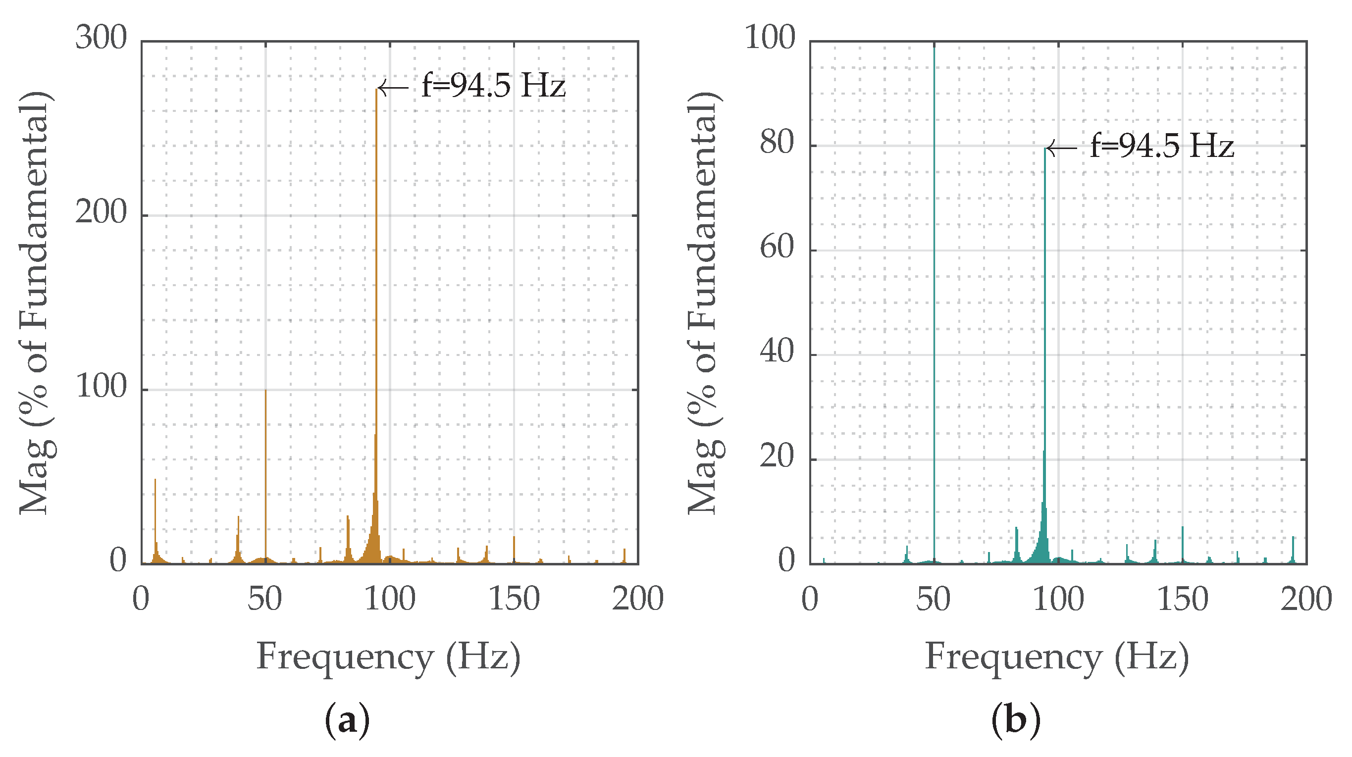
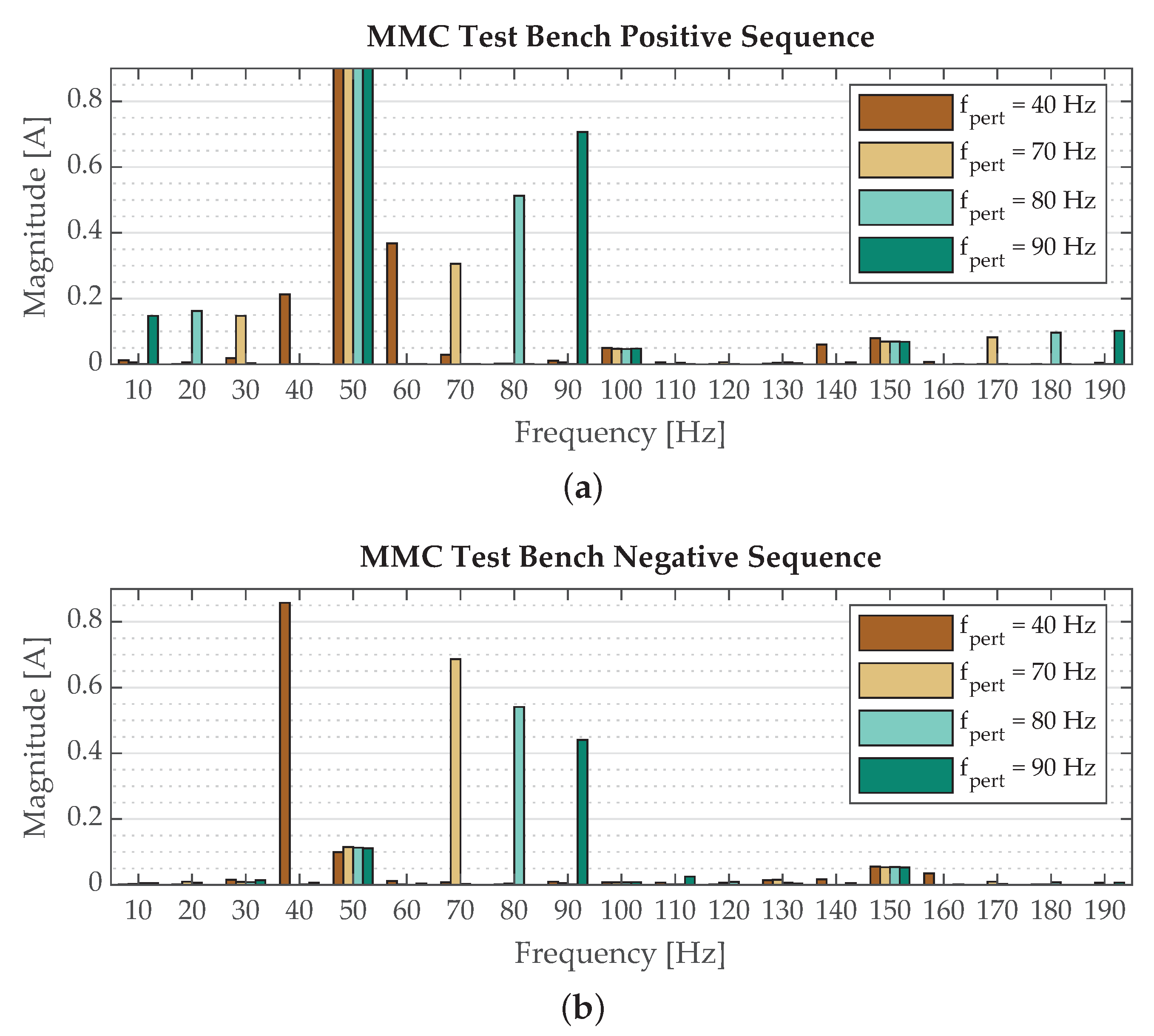
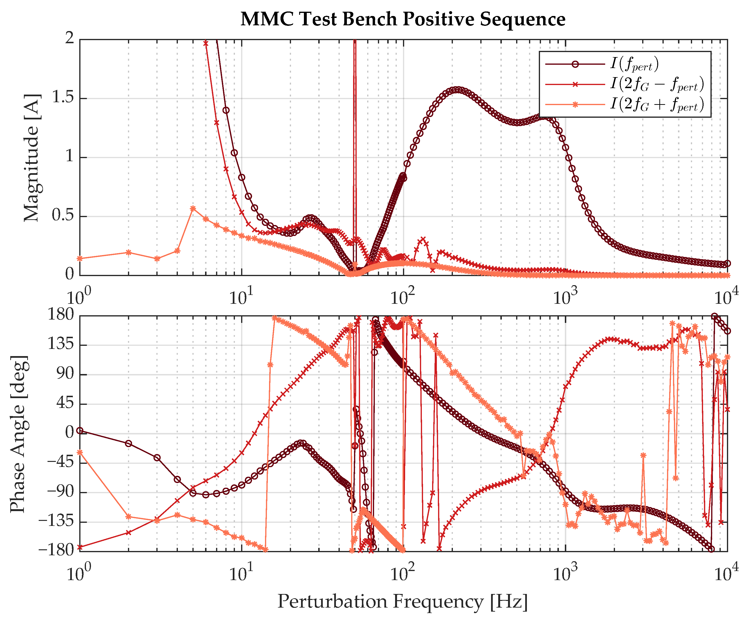
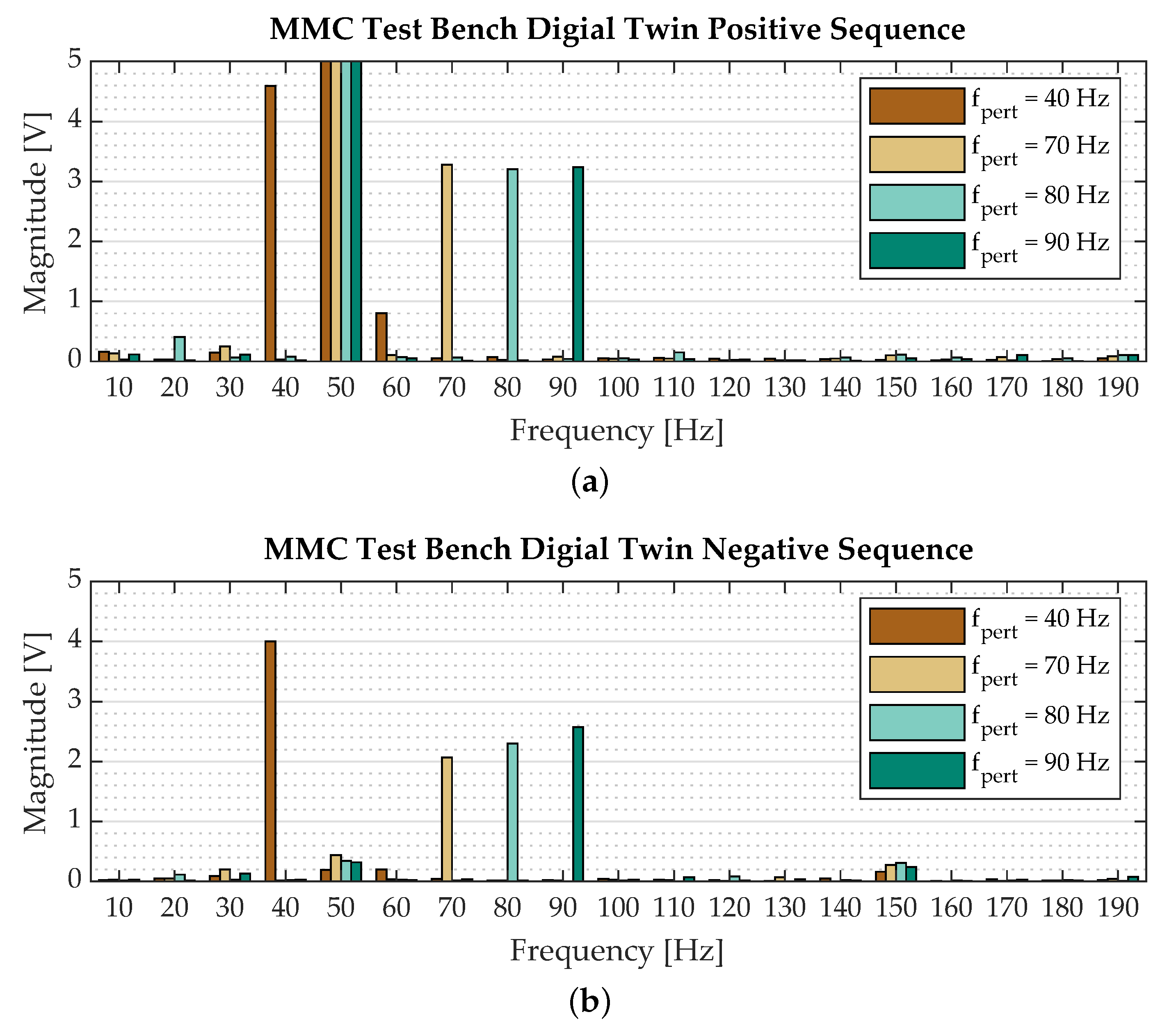
3.1. Spectrum Analysis

The impedance derivation method introduced in Section 2.2 is applied to measure the impedance of the MMC TB converters. A preceding analysis investigates the spectrum of the MMCs signals to determine with what frequencies the MMC TB responds to a perturbation. When operating in grid-following control mode, the MMC is perturbed by a voltage source, causing the converter to respond with a current. Therefore, the voltage injection approach shown in in Figure 4 is used and power amplifier 2 operates in voltage mode as shown in Figure 13. Applying a voltage perturbation at 40 Hz , 70 Hz , 80 Hz and 90 Hz , the corresponding current spectrum is analyzed. Figure 14 shows the effect of the perturbations on the current spectrum. As expected, the converter also responds with a current at 40 Hz , 70 Hz , 80 Hz and 90 Hz . However, for positive-sequence perturbations, the spectrum depicted in Figure 14a also contains current responses at 60 Hz and 140 Hz for a 40 Hz perturbation, at 30 Hz and 170 Hz for a 70 Hz perturbation, at 20 Hz and 180 Hz for a 80 Hz perturbation, and at 10 Hz and 190 Hz for a 90 Hz perturbation. In fact, for a 40 Hz perturbation, the response at 60 Hz exceeds that at 40 Hz , indicating a high degree of coupling in that frequency region. The results indicate a pattern in the current responses. When being subjected to a voltage perturbation with f = f p e r t , the MMC responds with a current with f = 100   Hz 2 f p e r t and f = 100   Hz + 2 f p e r t in addition to a current at f = f p e r t .
These currents are referred to as (mirror) frequency coupling [29,39,46] and are subsequently defined as a negative and positive coupling current dependent on the grid frequency fG and the perturbation frequency f p e r t with
f p e r t = 2 f G f p e r t
and
f p e r t + = 2 f G + f p e r t .
Due to nonlinearities of controllers, converters respond to a perturbation frequency with harmonics at frequencies other than the perturbation frequency. These harmonics can be identified in the dq-domain when the nondiagonal elements in a dq-domain impedance matrix are not zero and cross-couplings exist [28,32]. This coupling effect is typical for VSC including MMCs [39,47]. It can be caused by the grid frequency used in the dq-transformation of the converters’ control systems [5]. In particular, controllers that control the d- and q-axis current differently, such as the tracking controllers of the PLL, can be responsible for causing the coupling frequencies [46]. The effect was seen in STATCOM measurements in the China Southern Grid [5]. The PLL was considered responsible for transforming a component at the frequency f into two simultaneous components in the stationary frame, one at f G f and the other at f G + f [5]. However, different parts of the control system, such as the PWM, can also produce the coupling currents [48].
The spectrum depicted in Figure 14b, shows that no significant current magnitudes at frequencies other than the perturbation frequency can be seen for a negative-sequence perturbation.
Figure 15 shows the perturbation response current I ( f p e r t ) as well as the previously identified coupling currents I ( 2 f G f p e r t ) and I ( 2 f G + f p e r t ) when the MMC TB is subjected to a perturbation voltage source with frequencies ranging from 1 Hz to 10 k Hz . This means that for instance, for a perturbation frequency with f = 40 Hz the current response at 40 Hz , at 60 Hz , and at 140 Hz can be seen in the Bode plot. The current trajectories reveal that the current’s magnitude at f = f p e r t + is significantly smaller than at f = f p e r t . Furthermore, the plot shows that the frequency coupling effect is only significant at frequencies close to the grid frequency. However, as already seen in the spectrum analysis, the current response at f p e r t exceeds that at the perturbation frequency between 30 Hz and 60 Hz . The response at the coupling frequencies converges to zero for higher frequencies, and the MMC responds with the current at f p e r t only.
When operating in grid-forming control mode, the converter is perturbed with a current source and responds with a voltage. In this case, the current injection approach shown in Figure 4 is used and power amplifier 2 operates in current mode as shown in Figure 13. The converter reacts only with voltages at f p e r t as it can be seen in the voltage spectrum in Figure A2 of the Appendix A.
To conclude, the coupling current is only significant for the given system when
  • the MMC operates in grid-following control mode,
  • the MMC is subjected to a positive-sequence perturbation,
  • the perturbation frequency is below 200 Hz .

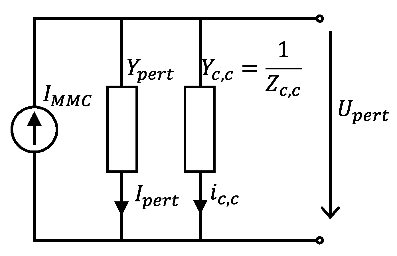
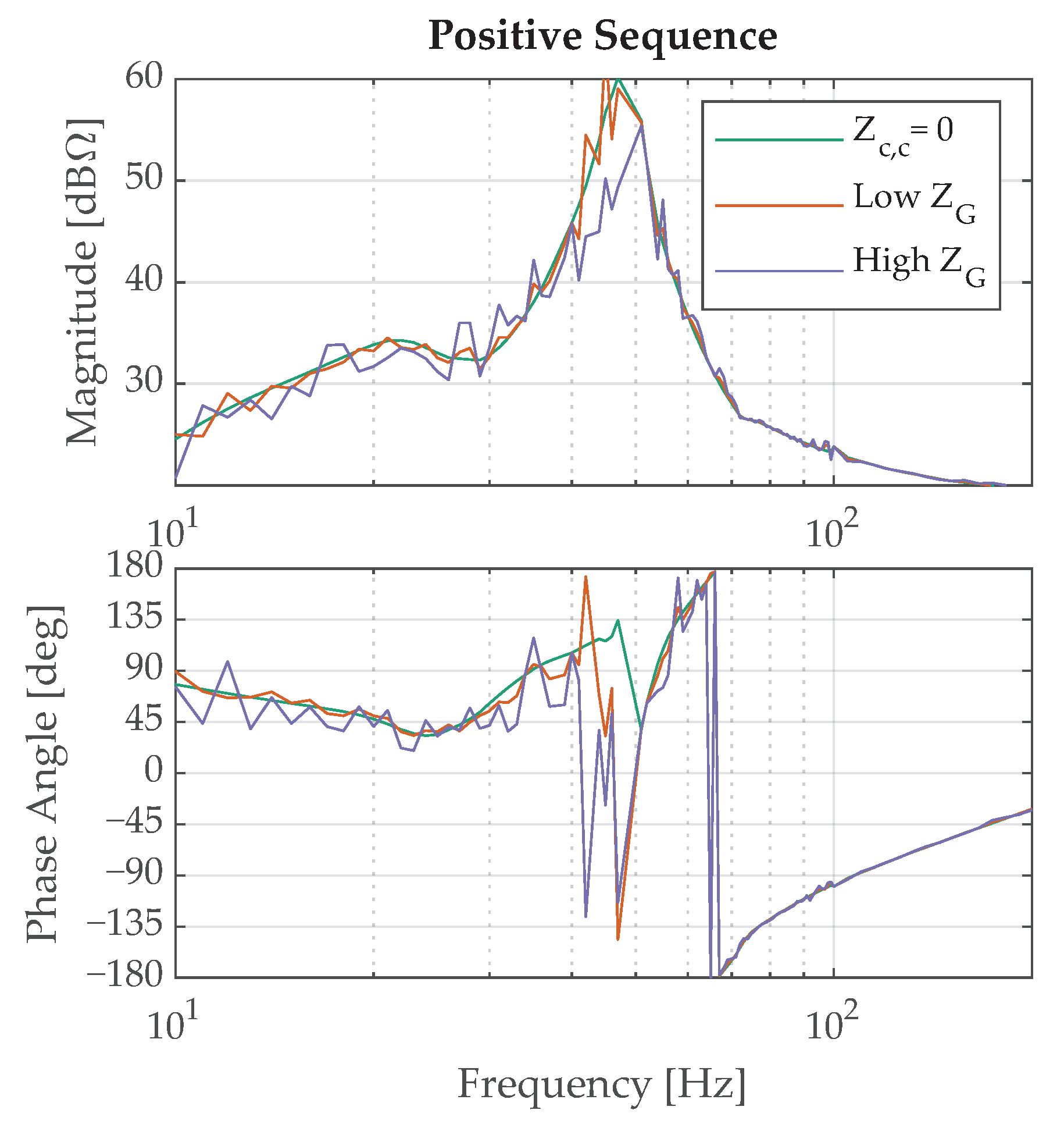
3.2. Coupling Modeling

As demonstrated in the previous section, the MMC responds to a positive-sequence voltage perturbation at f p e r t not only with a current at the same frequency but also with a current at f = 2 f G f p e r t when operating in grid-following control mode. Figure 16 illustrates how the additional current introduces a dependency of the grid impedance on the measured current response at f p e r t .
The voltage perturbation U p e r t ( f p e r t ) causes a current response at the same frequency, I p e r t ( f p e r t ) , and also one at the coupling frequency, i c ( 2 f G f p e r t ) , as seen in the spectrum analysis. This current leads to an additional voltage u c ( 2 f G f p e r t ) whose magnitude depends on the grid strength and the resulting grid impedance through the grid impedance. This voltage can be interpreted as an additional perturbation source that causes a current response at the same frequency, which is 2 f G f p e r t . Additionally, the converter also responds to the additional perturbation u c with a current i c , c at frequency
f = 2 f G ( 2 f G f p e r t ) = f p e r t .
As a result, the current response at f = f p e r t consists of the converter response to the voltage perturbation U p e r t ( f p e r t ) and that to the additional voltage perturbation u c ( 2 f G f p e r t ) . The latter introduces a nondesirable dependency of the converter impedance on the grid impedance, which nullifies the advantage of the IbSC that both subsystems’ impedances can be independently derived. While the measurement setup can include the grid impedance, this approach would further increase the required number of measurement series. Every grid impedance would require a new measurement; therefore, this approach is not feasible. Thus, the converter impedance is measured in ideal conditions, not including the grid impedance. The impact of the additional coupling current on the converter impedance can be subsequently included in the converter impedance model by an additional parallel impedance as presented in Figure 17 [39].
The additional impedance Z c , c ( f ) depends on the grid impedance as well as the additional current i c , c and is added in parallel to the converter impedance Z M M C . For simplification, it will be derived as the admittance Y c , c so that the overall converter admittance
Y M M C ( f p e r t ) = I p e r t ( f p e r t ) + i c , c ( f p e r t ) U p e r t ( f p e r t ) = I p e r t ( f p e r t ) U p e r t ( f p e r t ) Y p e r t + i c , c ( f p e r t ) U p e r t ( f p e r t ) Y c , c ( f p e r t ) .
The admittance Y c , c is derived on the basis of the model presented in [49] which maps the current i c ( 2 f G f p e r t ) to the perturbation voltage U p e r t ( f p e r t ) by defining a admittance
Y c ( f p e r t ) = i c ( 2 f G f p e r t ) U p e r t ( f p e r t ) .
Figure 16 illustrates that the current i c ( 2 f G f p e r t ) leads to a voltage u c ( 2 f G f p e r t ) through the parallel converter and grid and converter admittance so that
u c ( 2 f G f p e r t ) = i c ( 2 f G f p e r t ) Y p e r t ( 2 f G f p e r t ) + Y G ( 2 f G f p e r t ) .
The converter responds to this additional perturbation with the current i c , p at the same frequency and also with a second coupling current i c , c at frequency f = f p e r t as derived in (12). It can be expressed by
i c , c ( f p e r t ) = Y c ( 2 f G f p e r t ) · u c ( 2 f G f p e r t ) .
Replacing i c , c ( f p e r t ) in the right summand of (13) by (16) gives
Y c , c = Y c ( 2 f G f p e r t ) · u c ( 2 f G f p e r t ) U p e r t ( f p e r t ) .
Now u c ( 2 f G f p e r t ) in (17) can be represented by (15) so that
Y c , c = Y c ( 2 f G f p e r t ) U p e r t ( f p e r t ) · i c ( 2 f G f p e r t ) Y p e r t ( f p e r t ) + Y G ( 2 f G f p e r t ) .
Then Y c as in (14) can be used to replace i c ( 2 f G f p e r t ) U p e r t ( f p e r t ) in (18) which results in
Y c , c ( f p e r t ) = Y c ( 2 f G f p e r t ) · Y c ( f p e r t ) Y p e r t ( 2 f G f p e r t ) + Y G ( 2 f G f p e r t ) ,
as in [49]. The resulting admittance considers the influence of the grid impedance by integrating the current i c , c ( f p e r t ) into the overall impedance model Z M M C ( f p e r t ) . Including the admittance Y c , c ( f p e r t ) into the overall impedance model requires recording also the signals i c ( 2 f G f p e r t ) and U p e r t ( f p e r t ) as shown in (14) and (19). Consequently, the impedance measurement method in [33] is extended to also record the voltage U p e r t at f p e r t and the coupling current i c at 2 f G f p e r t which can be seen in Figure 15. Equation (19) also shows that the converter admittance Y c and the grid admittance Y G need to be obtained also for the coupling frequency 2 f G f p e r t for deriving Y c , c ( f p e r t ) . Thus, the derived admittances are additionally shifted so that the corresponding values at 2 f G f p e r t can be added to the model.
Figure 18 shows the impact of including the coupling current in the overall MMC impedance model. A low SCR ( S C R = 2 ) and consequently high grid impedance Z G significantly influences the MMC impedance trajectory at frequencies below 50 Hz . A higher SCR ( S C R = 6 ) shows a significantly reduced impact with the overall impedance almost matching the impedance when no coupling is modeled and Z c , c = 0 . Figure 18 also demonstrates that the coupling current does not affect the overall impedance at higher frequencies. Therefore, the coupling current is neglected in the impedance modeling for frequencies higher than 200 Hz .

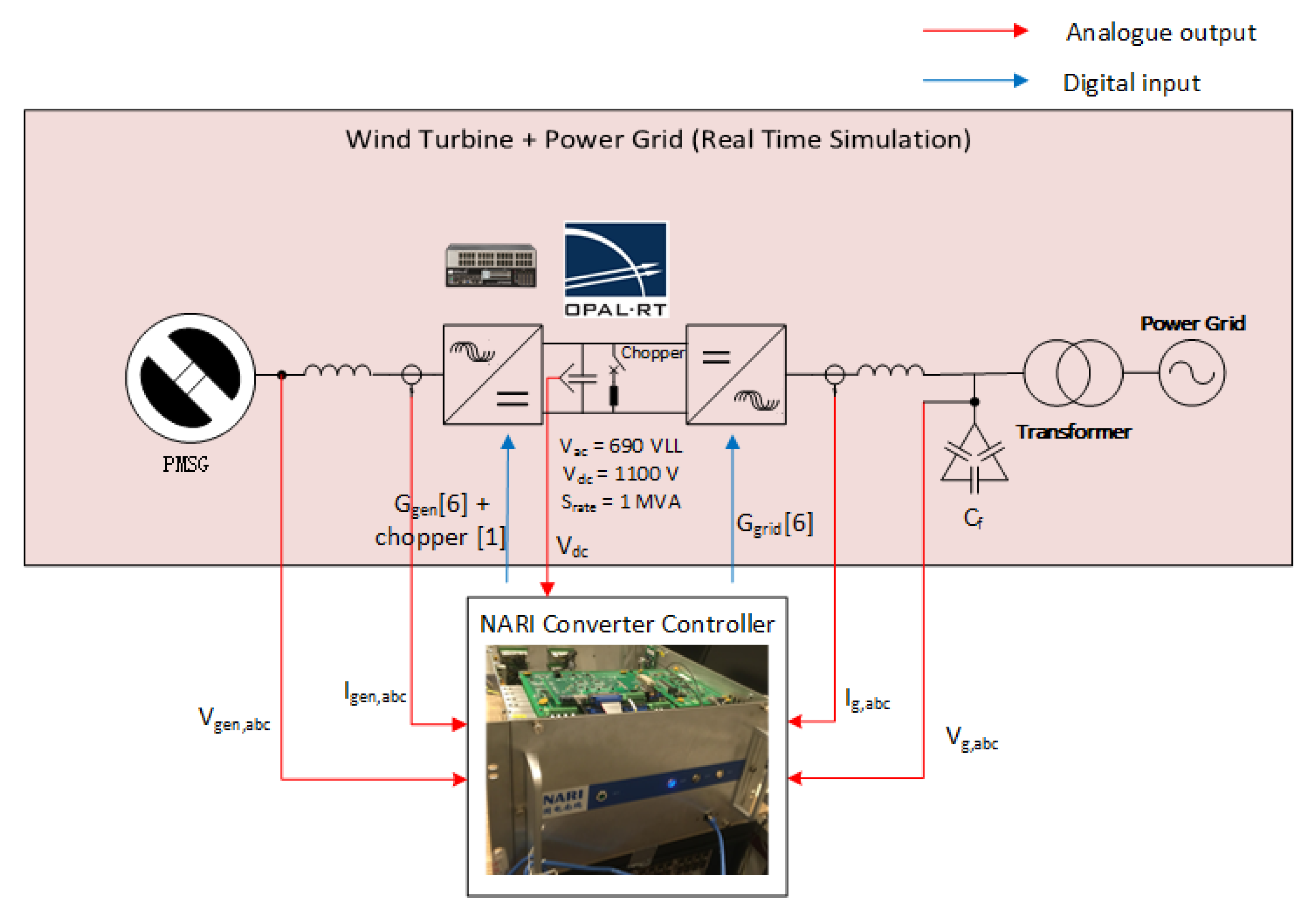
4. WT VSC Controller Replica System

The VSC of the wind turbine determines the frequency behavior of the offshore wind farm. The related impedance models are derived in the DNV GL Smart Grid Lab in Arnhem, The Netherlands. The goals of the laboratory are [40,41]:
  • To propose a PHiL test circuit to derive the impedance model of the power converter unit of a vendor-specific wind turbine (i.e., the power converter unit of a commercial 1 M W wind turbine generator). Further details for the PHiL TB can be found in [40].
  • To establish a CHiL TB to derive the impedance model a VSC WT controller replica that can be used for the grid integration of offshore wind power plants.
  • To compare the PHiL impedance of the VSC with its equivalent CHiL and provide suggested practices for potential industrial applications.
For this work, the CHiL impedance models the frequency behavior of the wind turbine VSC since it can be obtained with a higher bandwidth than the PHiL impedance. The CHiL TB depicted in Figure 19 is configured with the following key components:
  • The OPAL-RT real-time simulator consisting of OP5700.
  • A 1 M W WT VSC controller replica from Ming Yang Wind Power, Zhongshan, Guangdong, China.
The real-time simulator OPAL-RT OP5700 is the core of the system. It simulates a single wind turbine, including a wind turbine’s electrical subsystem, the generator, filters, transformer, the offshore AC-grid, and breakers. The simulations are FPGA-based. The MingYang Wind Power WT VSC controller replica connects to the OP5700 system through digital and analog channels [40,41]. The real-time simulator measures the grid side current and voltage signals I g , a b c and V g , a b c and the generator side current and voltage signals I g e n , a b c and V g e n , a b c . The analog output interface exports the signals. The OP5700 communicates with the WT VSC controller replica through 10 V analog signals. The controller replica then measures the terminal voltage and current coming from the controller replica. Using its time-stamped digital input interface, the OP5700 can interface with the controller replica’s measured signals. The resulting dq-impedance models used for the stability analysis are transformed into the sequence domain [50] and adjusted for outliers [45].

5. Stability Analysis

Using the scaled MMC TB and the WT VSC controller impedances, the converter-driven stability of a wind farm connected to the AC onshore grid by an HVDC link is assessed. Figure 20 depicts the investigated system.
The AC onshore grid is connected to an MMC operating in grid-following control mode and controlling the DC voltage. At the same time, the offshore wind farm is synchronized with an MMC operating in grid-forming control mode and providing the AC voltage magnitude and frequency. Thus, two test cases are defined to assess the stability of the system. The onshore test case investigates interactions between the AC onshore grid and the grid-following MMC and the offshore test case investigates interactions between the grid-forming MMC and the offshore wind farm. 600 M W are transmitted from the offshore wind farm to the shore, meaning that the impedance models are derived for 0.5 pu active power setpoint.

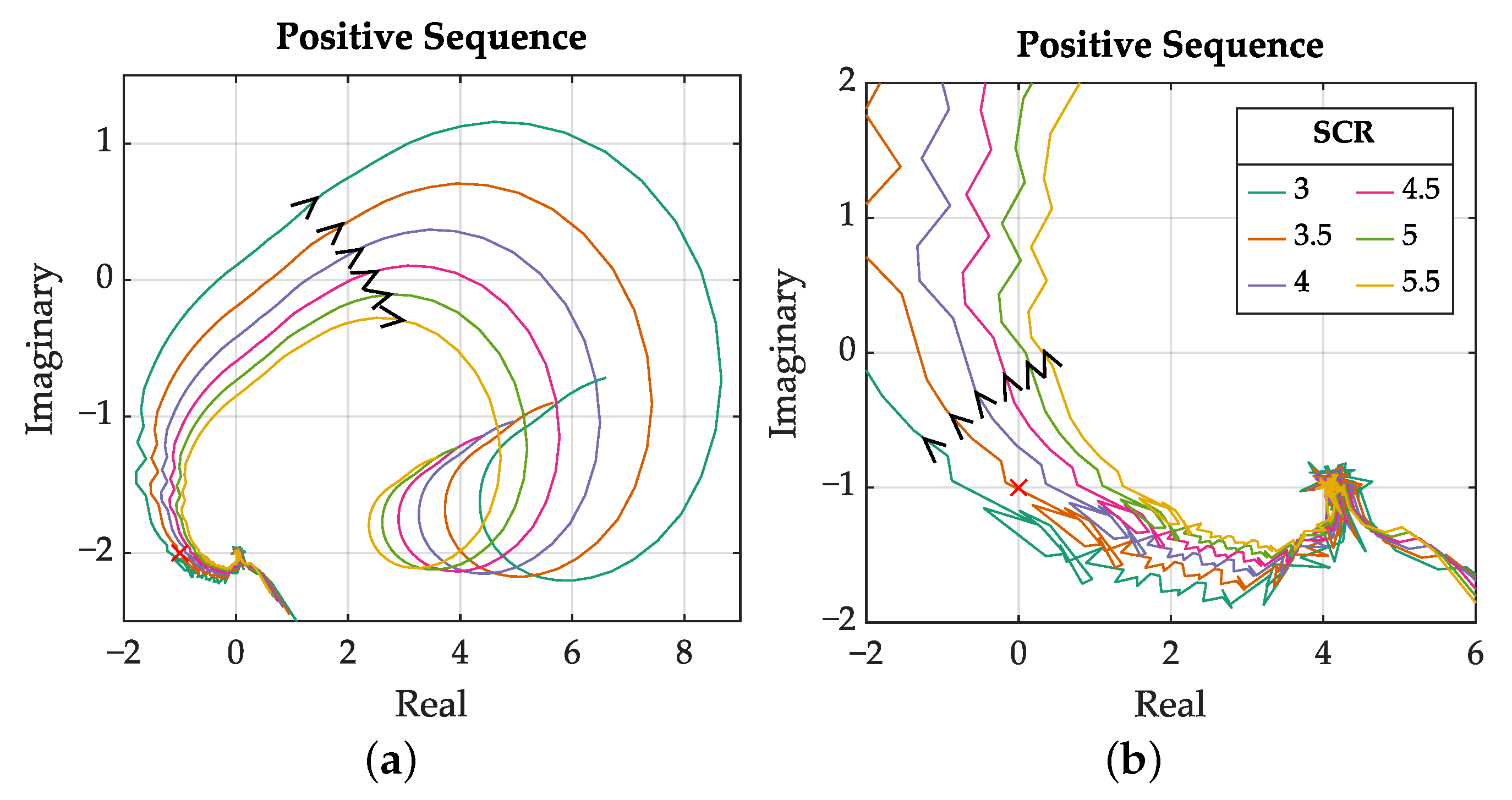
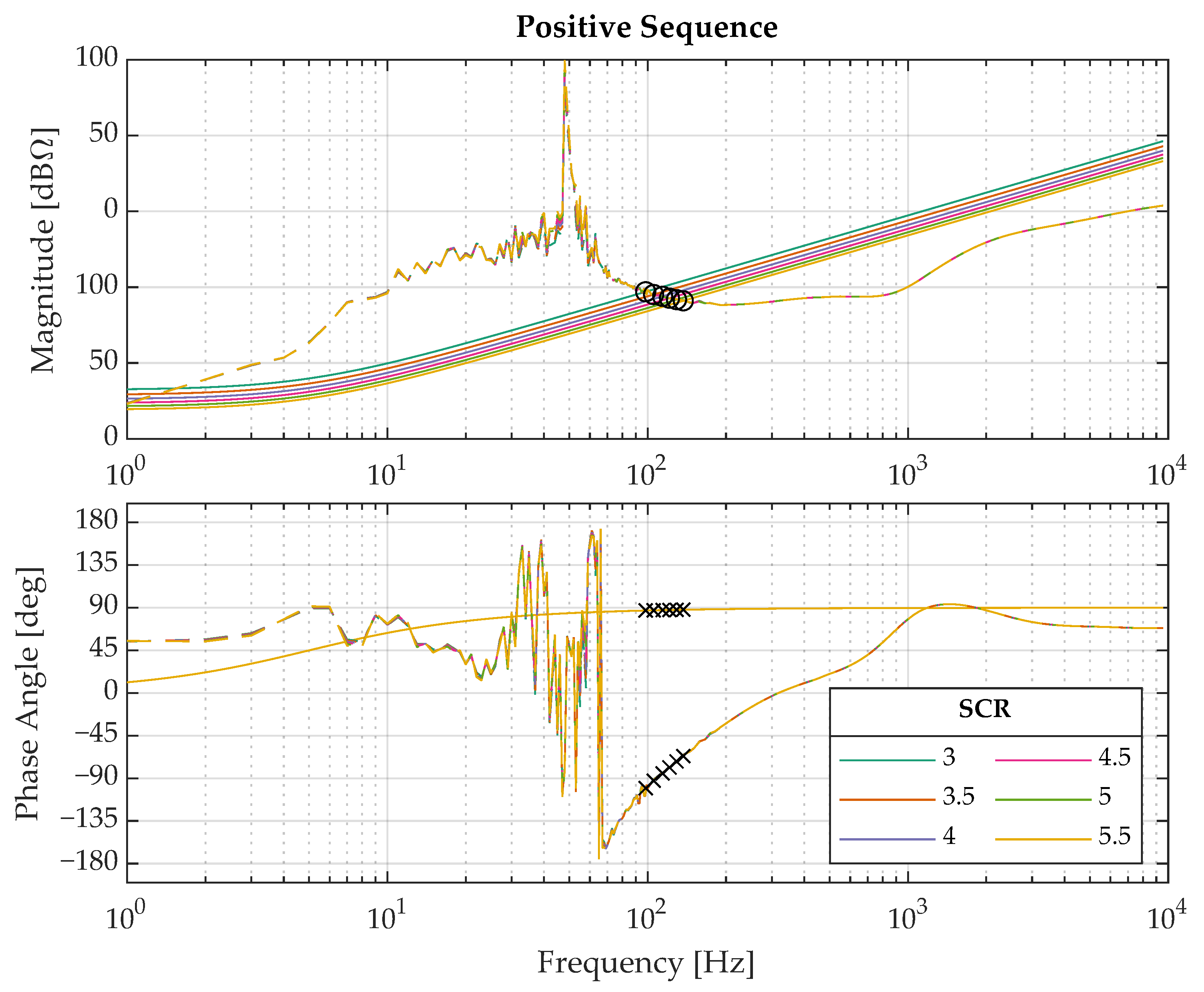
5.1. Onshore Test Case

Similar to the validation test case, different SCR are defined to investigate AC onshore grids with varying grid strengths. Investigating the positive-sequence impedance ratio first, Figure 21 depicts the positive-sequence Nyquist plots of the impedance ratio Z G ( f ) / Z M M C ( f ) with Figure 21b showing a close-up around the ( 1 , j 0 ) point.
The Nyquist plots show that for an S C R = 3.5 , the ( 1 , j 0 ) point is encircled, indicating an unstable system. The Bode plots in Figure 22 further reveal that the phase difference of the AC grid and MMC impedances reaches 180° for S C R = 3.5 and below.
Figure 23 depicts the Nyquist plots of the negative-sequence impedance ratio. They show that for the negative-sequence impedance ratio, the ( 1 , j 0 ) point is not encircled for the examined AC grid impedances. The Bode plots in Figure 24 show that even for an S C R = 3 , the phase difference does not exceed 180°.
To determine the onshore system’s overall stability and its proximity to instability, Table 5 presents the minimum PMs of the positive- and negative-sequence systems. Figure 18 shows that the effect of the additional coupling impedance is mainly relevant at frequencies around the grid frequency. Hence, the resulting PM do not differ for this particular case. Table 5 shows a negative and zero PM for the positive-sequence systems with S C R = 3 and 3.5 . Thus, the frequency-domain stability assessment demonstrates that already for a moderate SCR, the converter-driven stability is threatened due to unwanted interactions between the onshore MMC and the adjacent AC system.

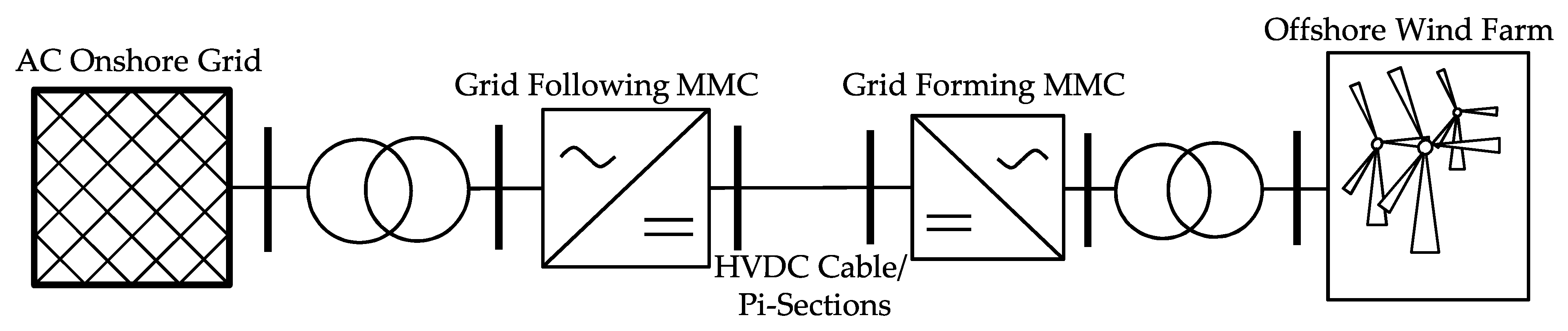
5.2. Offshore Test Case

The offshore test case investigates interactions between a grid-forming MMC and wind farm consisting of 600 wind turbines with 1 M W nominal power each. The WTs are arranged in a radial grid layout illustrated in Figure 25, showing also the equivalent circuit diagram of one radial line. The measured wind turbine impedance Z W T already includes the transformer impedance in addition to the converter impedance Z C . Additionally, the line impedance Z l with H = 0.3 mH is included in the wind farm model [51].
Consisting of m radial lines and n wind turbines in each line, the grid layout can be varied to investigate the topology’s impact on the stability. Thus, the overall wind farm impedance Z W F ( f ) is aggregated dependent on n and m using the aggregation algorithm developed in [52]. Considering an equal line impedance with Z l = Z l 1 = Z l 2 = Z l n , an equivalent admittance Y e q n is calculated according to I G of the equivalent circuit diagram with
Y e q n = Y W T + 1 Z l + 1 Y e q n 1 .
Starting with Y e q 1 = Y W T = 1 / Z W T ,
Y e q 2 = Y W T + 1 1 Y W T + Z l and Y e q 3 = Y W T + 1 1 1 1 Y W T + Z l + Y W T + Z l .
This formula is repeated until n is equal to the number of WT in a line. Considering more than one radial line, the overall wind farm impedance then equals to
Z W F = 1 m · Y e q n .
For the analysis, Z W F is determined for every possible grid configuration with n · m = 600 to ensure a power flow of 600 M W . As a result, the equivalent circuit diagram depicted in Figure 26 represents the offshore test case. Contrary to the validation and the onshore test case, not the MMC but the WT converters control the grid current. Therefore, a current source with parallel impedance represents the offshore wind farm. Operating in grid-forming control mode, the MMC provides the AC voltage and is therefore represented by a voltage source with series impedance.
Deriving the equivalent loop gain accordingly, the impedance ratio Z M M C ( f ) Z W F ( f ) is assessed for every wind farm grid layout with n · m = 600 and n , m N . The Nyquist plots in Figure 27 show a close-up of a part of the investigated grid layouts. For example, n , m = 600 , 1 shows a layout with 600 WT in one line while n , m = 1600 , shows the layout for 600 radial lines with one WT each. The Nyquist plots reveal that the different grid layouts do not result in an unstable system as the ( 1 , j 0 ) point is not encircled for positive- and negative-sequence impedance ratios. For further analysis Figure 28 shows the Bode plots of the grid-forming MMC’s impedances and those of the wind farm.
The plots show that the wind farm impedance magnitudes do not intersect those of the MMC. Thus, no PM close to zero can occur, and the system is stable for all grid configurations. Nevertheless, the offshore test case demonstrates that different grid layouts result in varying Nyquist and Bode plots. Therefore, the wind farm grid layout needs to be considered for the stability of the offshore system. The offshore system’s stability analysis also demonstrates that the IbSC and measurement-based impedance models are suitable for industrial applications, allowing that the models be derived independently and exchanged without sharing crucial information about the controllers.

6. Conclusions

In this paper, enhanced frequency-dependent impedance models are successfully derived for laboratory MMCs. Along with the previous work on the impedance model of a WT VSC controller replica [41], the developed impedance models were used to investigate the converter-driven stability of an MMC HVDC connected offshore wind park using the IbSC. The results indicate that couplings between frequencies and their impact are highly dependent on the converters’ control system. Thus, preliminary spectrum analyses are recommended for the impedance derivation. However, the implications and significance of couplings for stability assessments in industrial applications still merit investigation. For the investigated test cases, the identified coupling currents do not impact the stability assessments. Because the coupling currents depend on the applied control system, it is recommended to identify these currents and their relevance before the stability assessment when investigating different control systems. The work demonstrates that no confidential knowledge of the components needs to be shared among owners of different subsystems, e.g., wind turbines and MMCs, for assessing the system’s stability. Due to significantly reduced computation times compared to EMT time-domain simulations, the converter-driven stability of multiple scenarios can be investigated effectively. The onshore system results demonstrate that an MMC synchronized through a PLL with the AC onshore grid can experience converter-driven stability issues already at a moderate SCRs. Investigating various offshore grid layouts reveals that the stability assessment also depends on the grid topology; varying the grid layouts results in significantly different impedance models of the whole wind farm. Hence, impedance aggregation algorithms need to be appropriately considered. While the offshore test case demonstrates a stable system for all grid configurations, the converter-driven stability also depends on the control systems of the converters. Therefore, each analysis should consider the actual converter controls so that potential unstable scenarios are not overlooked.

Author Contributions

Conceptualization, M.Q., F.L., and Y.Y.; methodology, M.Q., F.L., O.E.A., and Y.Y.; investigation, M.Q., F.L. and Y.Y.; resources, F.L. and Y.Y.; writing—original draft preparation, M.Q. and L.N.; writing—review and editing, M.Q., F.L., Y.Y., and L.N.; visualization, M.Q. and L.N.; supervision, A.M.; project administration, A.M.; All authors have read and agreed to the published version of the manuscript.

Funding

The authors’ work has received funding from the European Union’s Horizon 2020 research and innovation program under grant agreement No 691714.

Conflicts of Interest

The funders had no role in the design of the study; in the collection, analyses, or interpretation of data; in the writing of the manuscript, or in the decision to publish the results. The authors declare no conflict of interest.

Abbreviations

The following abbreviations are used in this manuscript:
ACAlternating Current
CHiLControl Hardware in the Loop
DCDirect Current
DUTDevice Under Test
EMTElectromagnetic Transient
FPGAField Programmable Gate Array
HVDCHigh-Voltage Direct Current
IbSCImpedance-based Stability Criterion
MMCModular Multilevel Converter
MPMeasurement Parameters
NLMNearest-Level Modulation
PHiLPower Hardware in the Loop
PLLPhase-Locked Loop
PMPhase Margin
PWMPulse-Width Modulation
SCRShort-Circuit Ratio
SMSubmodule
STATCOMStatic Synchronous Compensator
TBTest Bench
TSOTransmission System Operator
VSCVoltage Source Converter
WTWind Turbine

Appendix A

Figure A1. Nyquist plots of AC grid and MMC impedance ratio of validation test case.
Energies 14 02341 g0a1
Figure A2. MMC TB digital twin voltage response spectrum with (a) positive-sequence and (b) negative-sequence current perturbation.
Energies 14 02341 g0a2

References

  1. Jovcic, D. High Voltage Direct Current Transmission; Wiley: Hoboken, NJ, USA, 2019. [Google Scholar] [CrossRef]
  2. Thomas, T. Troubleshooting Continues. VDE VERLAG GMBH. 2014. Available online: https://www.offshorewindindustry.com/news/troubleshooting-continues (accessed on 16 April 2021).
  3. Saad, H. Performance Analysis of INELFE Link with Control Replicas. RTE, Techreport. 2016. Available online: https://docs.google.com/viewer?a=v&pid=sites&srcid=ZGVmYXVsdGRvbWFpbnxodmRjcmVwbGljYXdvcmtzaG9wfGd4OjcwNjI1ZjBjMjJiNDRmODM (accessed on 16 April 2021).
  4. Saad, H.; Fillion, Y.; Deschanvres, S.; Vernay, Y.; Dennetière, S. On resonances and harmonics in HVDC-MMC station connected to AC grid. IEEE Trans. Power Deliv. 2017, 32, 1565–1573. [Google Scholar] [CrossRef]
  5. Shu, D.; Xie, X.; Rao, H.; Gao, X.; Jiang, Q.; Huang, Y. Sub- and super-synchronous interactions between STATCOMs and weak AC/DC transmissions with series compensations. IEEE Trans. Power Electron. 2018, 33, 7424–7437. [Google Scholar] [CrossRef]
  6. Hatziargyriou, N.; Milanović, J.V.; Rahmann, C.; Ajjarapu, V.; Cañizares, C.; Erlich, I.; Hill, D.; Hiskens, I.; Kamwa, I.; Pal, B.; et al. Stability Definitions and Characterization of Dynamic Behavior in Systems with High Penetration of Power Electronic Interfaced Technologies; Techreport PES-TR77; IEEE Power & Energy Society: Piscataway, NJ, USA, 2020. [Google Scholar]
  7. Wang, X.; Blaabjerg, F. Harmonic stability in power electronic based power systems: Concept, modeling, and analysis. IEEE Trans. Smart Grid 2018, 10, 2858–2870. [Google Scholar] [CrossRef] [Green Version]
  8. Buchhagen, C.; Greve, M.; Menze, A.; Jung, J. Harmonic Stability—Practical Experience of a TSO. In Proceedings of the 15th Wind Integration Workshop, Vienna, Austria, 15–17 November 2016. [Google Scholar]
  9. Sun, J.; Vieto, I.; Larsen, E.V.; Buchhagen, C. Impedance-Based Characterization of Digital Control Delay and Its Effects on System Stability. In Proceedings of the 20th Workshop on Control and Modeling for Power Electronics (COMPEL), Toronto, ON, Canada, 17–19 June 2019; pp. 1–8. [Google Scholar] [CrossRef]
  10. Rault, P.; Despouys, O. D9.3: BEST PATHS DEMO#2: Final Recommendations for Interoperability of Multivendor HVDC Systems; Technical Report; Best Paths: Madrid, Spain, 2018. [Google Scholar]
  11. Amin, M. Small-Signal Stability Characterization of Interaction Phenomena between HVDC System and Wind Farms. Ph.D. Thesis, Norwegian University of Science and Technology, Trondheim, Norway, 2017. [Google Scholar]
  12. Middlebrook, R.D. Input Filter Considerations in Designand Application of Switching Regulators. In Proceedings of the IEEE Industry Applications Society Annual Meeting, Chicago, IL, USA, 11–14 October 1976; pp. 366–382. [Google Scholar]
  13. Sun, J. Impedance-based stability criterion for grid-connected inverters. IEEE Trans. Power Electron. 2011, 26, 3075. [Google Scholar] [CrossRef]
  14. Sun, J.; Li, M.; Zhang, Z.; Xu, T.; He, J.; Wang, H.; Li, G. Renewable energy transmission by HVDC across the continent: System challenges and opportunities. CSEE J. Power Energy Syst. 2017, 3, 353–364. [Google Scholar] [CrossRef]
  15. Cao, W. Impedance-Based Stability Analysis and Controller Design of Three-Phase Inverter-Based AC Systems. Ph.D. Thesis, University of Tennessee, Knoxville, TN, USA, 2017. [Google Scholar]
  16. Sun, J.; Liu, H. Sequence impedance modeling of modular multilevel converters. IEEE J. Emerg. Sel. Top. Power Electron. 2017, 5, 1427–1443. [Google Scholar] [CrossRef]
  17. Love, G.N. Small Signal Modelling of Power Electronic Converters, for the Study of Time-Domain Waveforms, Harmonic Domain Spectra, and Control Interactions. Ph.D. Thesis, University of Canterbury, Electrical and Computer Engineering, Christchurch, New Zealand, 2007. [Google Scholar]
  18. Love, G.N.; Wood, A.R. Harmonic State Space model of power electronics. In Proceedings of the 2008 13th International Conference on Harmonics and Quality of Power, Wollongong, NSW, Australia, 28 September–1 October 2008; pp. 1–6. [Google Scholar] [CrossRef]
  19. Familiant, Y.A.; Huang, J.; Corzine, K.A.; Belkhayat, M. New techniques for measuring impedance characteristics of three-phase AC power systems. IEEE Trans. Power Electron. 2009, 24, 1802–1810. [Google Scholar] [CrossRef]
  20. Huang, J.; Corzine, K.A.; Belkhayat, M. Small-signal impedance measurement of power-electronics-based AC power systems using line-to-line current injection. IEEE Trans. Power Electron. 2009, 24, 445–455. [Google Scholar] [CrossRef]
  21. Bessegato, L.; Harnefors, L.; Ilves, K.; Norrga, S. A method for the calculation of the AC-side admittance of a modular multilevel converter. IEEE Trans. Power Electron. 2019, 34, 4161–4172. [Google Scholar] [CrossRef] [Green Version]
  22. Wu, H.; Wang, X. Dynamic impact of zero-sequence circulating current on modular multilevel converters: Complex-valued AC impedance modeling and analysis. IEEE J. Emerg. Sel. Top. Power Electron. 2019, 8, 1947–1963. [Google Scholar] [CrossRef]
  23. Wang, X.; Harnefors, L.; Blaabjerg, F. Unified impedance model of grid-connected voltage-source converters. IEEE Trans. Power Electron. 2018, 33, 1775–1787. [Google Scholar] [CrossRef] [Green Version]
  24. Bessegato, L.; Ilves, K.; Harnefors, L.; Norrga, S. Effects of control on the AC-side admittance of a modular multilevel converter. IEEE Trans. Power Electron. 2019, 34, 7206–7220. [Google Scholar] [CrossRef]
  25. Bayo Salas, A. Control Interactions in Power Systems with Multiple VSC HVDC Converters. Ph.D. Thesis, KU Leuven, Leuven, Belgium, 2018. [Google Scholar]
  26. Zhang, Y.; Chen, X.; Sun, J. Sequence impedance modeling and analysis of MMC in single-star configuration. IEEE Trans. Power Electron. 2020, 35, 334–346. [Google Scholar] [CrossRef]
  27. Wang, X.; Blaabjerg, F.; Wu, W. Modeling and analysis of harmonic stability in an AC power-electronics-based power system. IEEE Trans. Power Electron. 2014, 29, 6421–6432. [Google Scholar] [CrossRef]
  28. Bakhshizadeh, M.K.; Wang, X.; Blaabjerg, F.; Hjerrild, J.; Kocewiak, Ł.; Bak, C.L.; Hesselbæk, B. Couplings in phase domain impedance modeling of grid-connected converters. IEEE Trans. Power Electron. 2016, 31, 6792–6796. [Google Scholar] [CrossRef]
  29. Dowlatabadi, M.B. Harmonic Modelling, Propagation and Mitigation for Large Wind Power Plants Connected via Extra Long HVAC Cables: With special focus on harmonic stability. Ph.D. Thesis, Aalborg Universitetsforlag, Aalborg, Denmark, 2018. [Google Scholar]
  30. Amin, M.; Molinas, M. Small-signal stability assessment of power electronics based power systems: A discussion of impedance- and eigenvalue-based methods. IEEE Trans. Ind. Appl. 2017, 53, 5014–5030. [Google Scholar] [CrossRef]
  31. Vieto, I.; Sun, J. On system modeling and analysis using DQ-frame impedance models. In Proceedings of the 2017 IEEE 18th Workshop on Control and Modeling for Power Electronics (COMPEL), Stanford, CA, USA, 9–12 July 2017. [Google Scholar] [CrossRef]
  32. Xiao, Q.; Mattavelli, P.; Khodamoradi, A.; Tang, F. Analysis of transforming dq impedances of different converters to a common reference frame in complex converter networks. CES Trans. Electr. Mach. Syst. 2019, 3, 342–350. [Google Scholar] [CrossRef]
  33. Quester, M.; Loku, F.; Yellisetti, V.; Puffer, R. Online Impedance Measurement of a Modular Multilevel Converter. In Proceedings of the 2019 IEEE PES Innovative Smart Grid Technologies Europe (ISGT-Europe), Bucharest, Romania, 29 September–2 October 2019; pp. 1–5. [Google Scholar] [CrossRef]
  34. Quester, M.; Loku, F.; Yellisetti, V.; Moser, A. Frequency Behavior of an MMC Test Bench System. In Proceedings of the 2020 6th IEEE International Energy Conference (ENERGYCon), Gammarth, Tunisia, 29 September–1 October 2020. [Google Scholar] [CrossRef]
  35. Middlebrook, R.D. Small-signal modeling of pulse-width modulated switched-mode power converters. Proc. IEEE 1988, 76, 343–354. [Google Scholar] [CrossRef]
  36. Liao, Y.; Wang, X. General Rules of Using Bode Plots for Impedance-Based Stability Analysis. In Proceedings of the 2018 IEEE 19th Workshop on Control and Modeling for Power Electronics (COMPEL), Padua, Italy, 25–28 June 2018. [Google Scholar] [CrossRef]
  37. Cespedes, M.; Sun, J. Impedance modeling and analysis of grid-connected voltage-source converters. IEEE Trans. Power Electron. 2014, 29, 1254–1261. [Google Scholar] [CrossRef]
  38. Liu, H. HVDC Converters Impedance Modeling and System Stability Analysis. Ph.D. Thesis, Rensselaer Polytechnic Institute, Troy, NY, USA, 2017. [Google Scholar]
  39. Sun, J.; Wang, G.; Du, X.; Wang, H. A theory for harmonics created by resonance in converter-grid systems. IEEE Trans. Power Electron. 2019, 34, 3025–3029. [Google Scholar] [CrossRef]
  40. Sun, Y.; Perez, A.N.F.; Yang, Y.; Burstein, A.W.; de Jong, E.C.W.; Tang, B. PROMOTioN Work Package 16 Harmonic Resonance Demonstrator: Wind Turbine Generator Input-Impedance Measurement in DQ Frame. In Proceedings of the 18th Wind Integration Workshop, Dublin, Ireland, 16–18 October 2019. [Google Scholar]
  41. Ruffing, P.; Loku, F.; Quester, M.; Yang, Y.; Harson, A.; Burstein, A.; Sun, Y.; Fabian, A. Deliverable 16.3: Overview of the Conducted Tests, the Results and the Associated Analyses with Respect to the Research Questions and Analyses within WP3; Technical Report, PROMOTioN Project; PROMOTioN—Progress on Meshed HVDC Offshore Transmission Networks: Arnhem, The Netherlands, 2020. [Google Scholar]
  42. Cigré Working Group B4.57. Guide for the Development of Models for HVDC Converters in a HVDC Grid; CIGRE: Paris, France, 2014. [Google Scholar]
  43. Ruffing, P.F. HVDC Grid Protection Based on Fault Blocking Converters. Ph.D. Thesis, RWTH Aachen University, Aachen, Germany, 2020. [Google Scholar] [CrossRef]
  44. Van Hertem, D. HVDC Grids: For Offshore and Supergrid of the Future; IEEE Press: Piscataway, NJ, USA; Wiley: Hoboken, NJ, USA, 2016. [Google Scholar]
  45. Loku, F.; Quester, M.; Wienkamp, P.; Kaiser, M.; Ruffing, P.; Bernal-Perez, S.; Martínez, J.; Blasco-Gimenez, R.; Arasteh, A.; Jahn, I.; et al. Deliverable 16.4—Test Case Analysis; Technical Report, PROMOTioN Project; PROMOTioN—Progress on Meshed HVDC Offshore Transmission Networks: Arnhem, The Netherlands, 2020. [Google Scholar]
  46. Rygg, A. Impedance-Based Methods for small-Signal Analysis of Systems Dominated by Power Electronics. Ph.D. Thesis, Norwegian University of Science and Technology, Trondheim, Norway, 2018. [Google Scholar]
  47. Vieto, I.; Huang, P.; Reinikka, T.; Nademi, H.; Buchhagen, C.; Sun, J. Online Measurement of Offshore Wind Farm Impedance for Adaptive Control of HVDC Transmission Systems. In Proceedings of the 2019 20th Workshop on Control and Modeling for Power Electronics (COMPEL), Toronto, ON, Canada, 17–20 June 2019; pp. 1–8. [Google Scholar] [CrossRef]
  48. Yang, D.; Wang, X.; Blaabjerg, F. Sideband harmonic instability of paralleled inverters with asynchronous carriers. IEEE Trans. Power Electron. 2018, 33, 4571–4577. [Google Scholar] [CrossRef]
  49. Vieto, I.; Sun, J. Sequence Impedance Modeling and Converter-Grid Resonance Analysis Considering DC Bus Dynamics and Mirrored Harmonics. In Proceedings of the 2018 IEEE 19th Workshop on Control and Modeling for Power Electronics (COMPEL), Padua, Italy, 25–28 June 2018; p. 8. [Google Scholar] [CrossRef]
  50. Sun, Y.; Ruffing, P.; Quester, M.; Bernal-Perez, S.; Añó-Villalba, S.; Yang, R.B.G.Y.; Dowlatabadi, M.K. Deliverable 16.5: Implementation of an Analytical Method for Analysis of Harmonic Resonance Phenomena; Technical Report, PROMOTioN Project; PROMOTioN—Progress on Meshed HVDC Offshore Transmission Networks: Arnhem, The Netherlands, 2019. [Google Scholar]
  51. Dowlatabadi, M.; Hjerrild, J.; Kocewiak, Ł.; Blaabjerg, F.; Bak, C. On Aggregation Requirements for Harmonic Stability Analysis in Wind Power Plants. In Proceedings of the 16th Wind Integration Workshop, Berlin, Germany, 25–27 October 2017. [Google Scholar]
  52. Quester, M.; Yellisetti, V.; Loku, F.; Puffer, R. Assessing the Impact of Offshore Wind Farm Grid Configuration on Harmonic Stability. In Proceedings of the 2019 IEEE Milan PowerTech, Milan, Italy, 23–27 June 2019. [Google Scholar] [CrossRef]
Figure 1. Equivalent circuit diagram of investigated system.
Energies 14 02341 g001
Figure 2. Equivalent circuit diagram represented as feedback loop.
Energies 14 02341 g002
Figure 3. Impedance measuring method overview.
Energies 14 02341 g003
Figure 4. Circuit diagram of the MMC impedance derivation setup.
Energies 14 02341 g004
Figure 5. MMC connected to AC grid.
Energies 14 02341 g005
Figure 6. Cascaded vector control scheme for controlling the MMC.
Energies 14 02341 g006
Figure 7. MMC impedance and AC grid impedance for different SCRs.
Energies 14 02341 g007
Figure 8. MMC impedance and AC grid impedance for different SCRs.
Energies 14 02341 g008
Figure 9. Close up of MMC and AC grid impedance intersections for (a) positive-sequence and (b) negative-sequence impedances.
Energies 14 02341 g009
Figure 10. AC terminal current when MMC is connected to AC grids with decreasing SCR.
Energies 14 02341 g010
Figure 11. AC terminal current (a) and voltage (b) when switched to an AC grid with SCR = 4.
Energies 14 02341 g011
Figure 12. Fourier spectrum of phase a of the AC terminal current (a) and voltage (b) when connected to an AC grid with SCR = 4.
Energies 14 02341 g012
Figure 13. MMC TB setup for the impedance derivation.
Energies 14 02341 g013
Figure 14. MMC TB current response spectrum with (a) positive-sequence and (b) negative-sequence perturbation.
Energies 14 02341 g014
Figure 15. MMC TB current response to a voltage perturbation with frequency f p e r t .
Energies 14 02341 g015
Figure 16. Influence of coupling current on measured current response.
Energies 14 02341 g016
Figure 17. MMC impedance model with additional coupling impedance.
Energies 14 02341 g017
Figure 18. MMC TB impedance with no coupling modeled ( Z c , c = 0 ), high SCR (low Z G ) and low SCR (high Z G ).
Energies 14 02341 g018
Figure 19. CHiL TB setup for the WT VSC controller replica impedance measurement.
Energies 14 02341 g019
Figure 20. HVDC system connecting offshore windfarm to AC system.
Energies 14 02341 g020
Figure 21. Complete (a) and zoomed (b) Nyquist plots of MMC in grid-following control mode and AC grid for different SCR with positive-sequence perturbation.
Energies 14 02341 g021
Figure 22. Bode plots of MMC in grid-following control mode and AC grid for different SCRs with positive-sequence perturbation.
Energies 14 02341 g022
Figure 23. Complete (a) and zoomed (b) Nyquist plots of MMC in grid-following control mode and AC grid with negative-sequence perturbation.
Energies 14 02341 g023
Figure 24. Bode plots of MMCs in grid-following control mode and AC grid for different SCR with negative-sequence perturbation.
Energies 14 02341 g024
Figure 25. Offshore wind farm grid layout with equivalent circuit diagram for one radial line.
Energies 14 02341 g025
Figure 26. Equivalent circuit diagram of offshore test case.
Energies 14 02341 g026
Figure 27. Nyquist plots of grid-forming MMC and offshore wind farm impedance ratio for different wind farm grid layouts.
Energies 14 02341 g027
Figure 28. Bode plots of grid-forming MMC and offshore wind farm impedance ratio for different wind farm grid layouts.
Energies 14 02341 g028
Table 1. Simulated MMC model parameters.
ParameterVariableValue
Converter power P n , M M C 1200 M W
DC voltage U D C , n 640 k V
Arm inductance L A r m 46.2 m H
Resistance arm inductance R A r m 0.08 Ω
On resistance R S M , o n 0.08 Ω
Number of SMs n S M 350
SM capacity C S M 8.8 m F
AC primary voltage U A C , 1 400 k V
AC secondary voltage U A C , 2 350 k V
Transformer reactance R A C , 1 0.31621 Ω
Transformer inductance L A C , 1 0.403 m H
Transformer reactance R A C , 2 0.726 Ω
Transformer inductance L A C , 2 0.92473 m H
Table 2. AC grid impedance parameters.
SCR S SC , G [GVA] R G [ Ω ] L G [mH]
44.83.3168105.58
56.02.653484.46
67.22.211270.38
78.41.895360.33
Table 3. Phase Margins for positive- and negative-sequence impedances.
SCR f P M , p o s P M p o s f P M , n e g P M n e g
491 Hz 10 172 Hz 17
5106 Hz 8 189 Hz 30
6119 Hz 20 208 Hz 41
7133 Hz 31 227 Hz 51
Table 4. MMC Test Bench parameters.
ParameterVariableValue
Nominal output power P n , M M C 6 k W
Nominal DC voltage U D C , n 400 V
Nominal DC current I D C , n 15 A
Nominal frequency f n 50 Hz
Nominal AC primary voltage (3-phase) U A C , 1 400 V (Line-to-line RMS)
Nominal AC secondary voltage (3-phase) U A C , 2 208 V (Line-to-line RMS)
Nominal AC RMS current at f n I A C , n 16.7 A
MOSFET switching frequency f s w 0–10 k Hz
Number of cells (submodules) n S M 10
Nominal cell voltage U c e l l , n 40 V
Cell capacitor C S M 4.92 m F
Arm inductor L A r m 2.5 m H
Transformer rated power S T r 8 k V A
Transformer vector group Y / Δ (Ynd11)
Table 5. Phase Margins of MMC in grid-following control mode and AC grid for different SCR.
SCR f pos [Hz] PM pos [deg] f neg [Hz] PM neg [deg]
395−81697
3.5105017915
4114819022
4.51211419928
51292020934
5.51372522040
Publisher’s Note: MDPI stays neutral with regard to jurisdictional claims in published maps and institutional affiliations.

