A Two-Dimensional Partitioning of Fracture–Matrix Flow in Fractured Reservoir Rock Using a Dual-Porosity Percolation Model

Abstract

Fractures and micropores have varying contributions to the gas permeability of fractured reservoirs. The quantification of the contribution of fractures and micropores that form a dual-porosity system for gas permeability is critical when attempting to accurately evaluate gas production. However, due to insufficient knowledge of fracture–matrix flow partitioning in such dual-porosity systems, it is challenging for previous models to quantitatively characterize the fracture heterogeneity and accurately evaluate the gas flow and permeability in fractured rocks. In this study, we propose a dual-porosity percolation model to quantitatively investigate the contributions of fractures and matrix micropores towards the gas permeability of fractured rocks. Using percolation theory, we establish fracture networks with complex heterogeneity, which are characterized by various fracture densities and percolation probabilities within a porous matrix with various fracture/matrix permeability ratios. The compressible Navier–Stokes and Brinkman equations were adopted to describe the gas flow in the fractures and porous matrix, respectively. The simulation results indicate that the gas permeability of the dual-porosity system has an exponential relationship with the fracture density and matrix permeability. The contribution of fractures and matrix micropores toward gas permeability can be classified by establishing a two-dimensional partitioning of the fracture–matrix flow related to the fracture heterogeneity and fracture/matrix permeability ratio. The contribution of matrix micropores cannot be neglected if the fracture density is lower than a critical value.

1. Introduction

Unconventional hydrocarbon reservoirs are characterized by low porosity and permeability [1,2]. Fracturing stimulations create a complex fracture network that connects numerous micropores in rock matrices, which dramatically increases the gas permeability of unconventional tight hydrocarbon reservoirs [3,4]. In general, hydraulic fractures and micropores in rock matrices contribute differently to the gas permeability in fractured reservoir rocks. Previous studies have shown that gas flows in fractures and porous matrices behave differently and have effects on each other [5,6,7]. The quantification of fracture and micropore contributions in the formation of dual-porosity systems in terms of gas permeation capabilities is critical to accurately evaluate unconventional gas production [6]. However, due to insufficient knowledge of fracture–matrix flow partitioning in such dual-porosity systems, previous studies have been unable to accurately quantify the gas flow and permeability of fractured rocks [5,8,9].

Hydraulic fractures connect the natural microfractures, micropores, and nanopores within a rock matrix in fractured reservoir rocks. They form the flow channels for fractured reservoir rocks after methane desorption from the organic nanopores and micropores [10,11,12]. Figure 1 shows a sketch map of the fractures and micropores within fractured reservoir rocks. Since hydraulic fractures are much larger than both micropores and nanopores in tight reservoir rocks, most of the previous studies have ignored the contributions of micropores to the gas permeability of reservoir rocks [13,14,15] and have mainly considered the fracture fluid flow when investigating the permeability of fractured rocks [16,17]. These studies assume that the reservoir medium is impermeable before fracture reconstruction, whereas fracture networks mainly dominate the permeability after fracturing. For nanopores and micropores, most previous studies have focused on the processes of gas adsorption, desorption, and diffusion in such structures [18,19,20,21]. However, gas flow in fractures and gas diffusion in matrices are different and have effects on each other in real fractured reservoirs. Rasmussen et al. [22] made several improvements by considering fluid flow in the rock matrix and discussed the effects of vertical fracture/matrix permeability ratios on fluid flow using the boundary element method (BEM). They considered fractures as a separate system from the matrices without taking into account the fluid flow from fractures to the matrix. Lough et al. [23] and Lee et al. [24] further improved the method suggested by Rasmussen et al. [22] and extended it to medium-sized fractures or larger fractures using the BEM. The influence of short fractures on matrix permeability was considered, while the effect of long fractures was not taken into account. Teimoori et al. [5] calculated the effective permeability in fractured reservoirs and concluded that the matrix permeability, fracture density, size, aperture, and interconnectivity all contribute to the effective permeability of an individual grid block. Recent studies [6,20,25] also suggested that these factors, especially the hydraulic fracture interconnections with micropores in the matrices, will directly affect the quantitative calculation of gas permeability of fractured rocks. Bai et al. [26] studied the dual-porosity behavior of naturally fractured reservoirs, taking into account the transient flow in the matrix blocks. Cai et al. [27] introduced a new modeling concept to numerically investigate the fracture–matrix interactions in shale gas reservoirs. The applications of new models are restricted to a few shape blocks and the universality of such models requires more tests and verifications. Wang et al. [28] formulated an analytical model to simulate real gas transport in nanopores and complex fractures in shale gas reservoirs and discussed the effect of multiple physics on the shale gas production, however the impact of fracture heterogeneity was not considered in their model. Abbasi et al. [29] proposed an analytical solution for fluid flow in a transient dual-porosity model and focused on investigating the influence of rock matrix block size in fractured formations. These studies attempted to simulate fracture–matrix interactions in tight fractured reservoirs from a variety of perspectives, but did not fully recognize or quantify fracture–matrix flow partitioning and its dependence on hydraulic fractures [3,30]. Nevertheless, Matthäi et al. [31] investigated numerical fluid flow partitioning between fractures and matrices based on field data and revealed the critical fracture aperture values that mark the transition from the matrix to fracture-dominated flow. Actually, the gas permeability in fractured rocks is not only related to the fracture aperture, but it intrinsically depends on the relative value of the fracture permeability to the matrix permeability. The three characteristic flow regimes were divided by their respective fracture–matrix permeability ratios (k_f/k_m), named fracture-dominated flow, fracture-perturbed flow, and fracture-negligible flow. Sanaee et al. [32] also numerically simulated fracture core flooding test data to investigate the flow partitioning between fracture and matrix systems, which is affected by the in situ stress regime in the reservoir. The results also revealed a flow transition of higher fluid permeability under the lower stress magnitudes and a negligible impact of fracture distribution when the fractures are compressed under higher loading pressure. The respective fracture–matrix permeability ratio changes with the fracture closure due to the increase of loading pressure. Although the flow transition was observed in the abovementioned dual-porosity model with fractures and micropores, the partitioning of fracture–matrix flow is ambiguous and there is a lack of quantitative parameters to accurately distinguish the contributions of fractures and matrix flow. It has been demonstrated that reservoir rock has a complex heterogeneous and discontinuous structure, which plays a vital role in fluid flow through fractured geological media [33,34]. Therefore, it is inaccurate to describe and classify the flow transition in the fractured rocks using only one-dimensional partitioning of the fracture/matrix permeability ratio k_f/k_m. To intuitively characterize the impacts of discontinuity heterogeneity and reveal the controlling mechanism of fluid flow in porous fracture–matrix media, it is crucial to establish two-dimensional partitioning of the fracture–matrix flow regarding the contributions of the gas flow in the matrix. Additionally, previous studies have often ignored Klinkenberg effects and gas compressibility when calculating the gas permeability of fractured reservoirs [5].

Since unconventional oil and gas reservoirs are often buried at depths of more than 3000 m [35], it is extremely difficult to detect and analyze gas flow in fractures and micropores in the matrix utilizing field tests. Additionally, it is also quite difficult to obtain rock core samples and measure gas flow during the fracturing process with exposure to real geological environments in the laboratory. Although the development of numerous laboratory methods has led to attempts to obtain the real dual-porosity structure in fractured reservoir rocks and discuss its influence on rock permeability, such as X-ray computed tomography (CT) [36,37,38] and scanning electron microscopy (SEM) techniques [39,40], it is nearly impossible to obtain a certain regular fracture system via experiments and quantitatively determine the statistical relationships between the pore space, fracture distribution, and equivalent permeability of fractured rocks using these methods. Another challenge to investigations of fractured reservoir permeability is that the fracture apertures and pore sizes are at various scales, which results in difficulties when attempting to quantitatively describe both the fluid flow in micropores and hydraulic fractures in fractured rock samples. Quantitative evaluation studies still face numerous obstacles, such as understanding the contributions of fractures and pores in matrices to gas flow at the core scale in the laboratory. Therefore, previous studies have adopted probabilistic methods and numerical simulation as alternatives, which are time-saving and flexible techniques that allow the construction of a pore–fracture system and an analysis of both the fluid flow in the pores and fractures of the fractured rock mass. Among them, the Monte Carlo method [41] is a widely used technique to simulate the fracture networks of rocks through a series of physical or geometrical statistical parameters. Combined with percolation theory, it is often used to investigate fluid flow through disordered porous media and tight reservoirs [42,43,44,45,46,47]. These studies mostly used simple line segments to obtain a graph of the fracture networks. The generation of most fracture networks requires large amounts of time, and few models accurately reconstruct the fracture while the heterogeneity, fracture length, fracture aperture, and random azimuth are simutaneously taken into account [25,45,48]. The complicated pattern of fracture networks is mainly determined by the number of fractures in a rock core, namely the fracture density. Zhang et al. [49] developed and extended the percolation theory to generate heterogeneous fracture networks with various fracture densities, fracture apertures, and random azimuths, which is applied in this study.

Intending to quantitatively investigate fracture–matrix flow partitioning in fractured rocks, in this study we developed a dual-porosity model to evaluate the gas permeability of tight rocks. The percolation theory was used to establish fracture networks with complex heterogeneity, which were characterized by various fracture densities and percolation probabilities. The facture networks were coupled with a porous matrix featuring various permeabilities, thereby leading to reconstructed structures with various fracture/matrix permeability ratios. We considered that gas flow not only occurs through connected fractures but also through the matrix micropores. Fractures and matrices were divided into two solution domains to simulate gas flow in fractured rocks using the compressible Navier-stokes (N–S) and Brinkman equations, respectively. The coupling flow in the matrix and fractures was simulated using the variable exchanges between the velocity and pressure fields. We adapted the methods reported by Zhang et al. [49] to build five sets of random fracture models with varying fracture densities using Monte Carlo simulation technology. The fracture connectivity was quantitatively studied using the percolation theory. A single-phase flow simulation was performed to mimic methane flow and calculate the equivalent gas permeability values of fractured rock models, considering gas compressibility and Klinkenberg effects. The same fracture networks (but with three matrix properties) were studied to quantitatively analyze the impacts of the fracture density and fracture/matrix permeability ratio on the equivalent permeability of fractured rocks. The contributions of fractures and matrix micropores to the gas permeability were classified through two-dimensional partitioning of fracture–matrix flow in porous media, considering the fracture heterogeneity and fracture/matrix permeability ratio. This study provides a modeling basis for evaluation of the permeability of unconventional oil and gas reservoirs.

2. Materials and Methods

This study used MATLAB to generate 2-D-connected fracture networks. The procedures included three steps: (1) five groups of fracture models with identical fracture densities but different fracture distributions were generated using the Monte Carlo method in MATLAB; (2) the fracture connectivity was analyzed based on percolation theory, whereby for fracture densities lower than the critical density, the permeable probability was zero; (3) for networks with a fracture density near or above the critical density, the system was considered to be permeable and we performed a compressible flow simulation to compute the methane flow in pores and fractures and determine the equivalent permeability according to Darcy’s law.

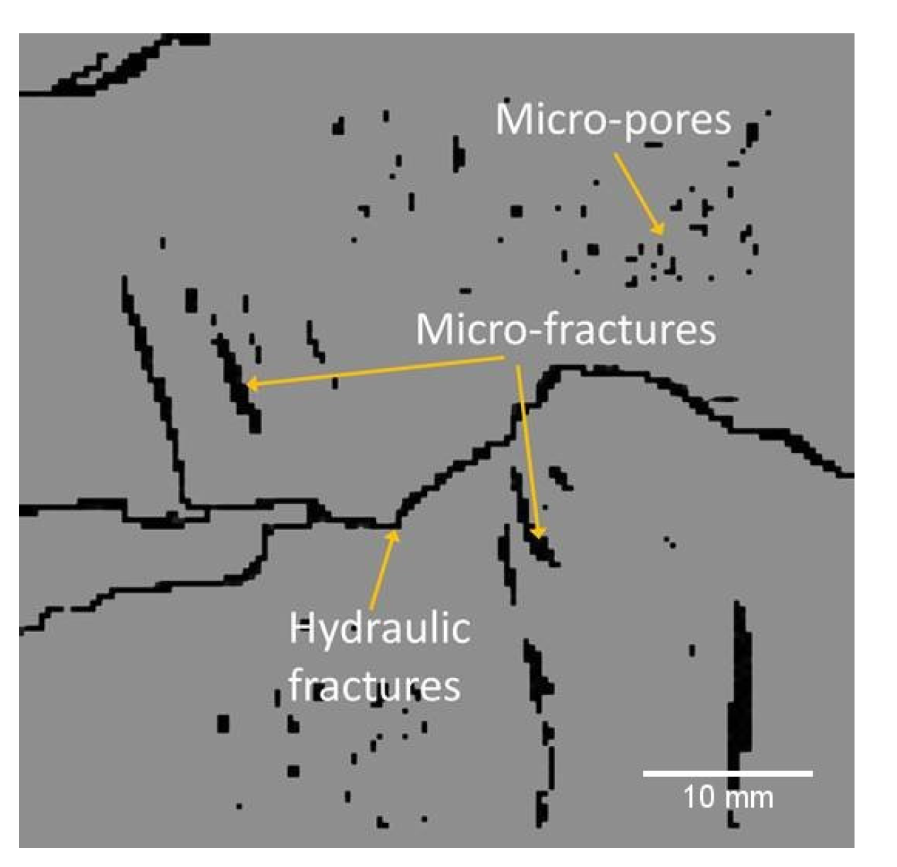
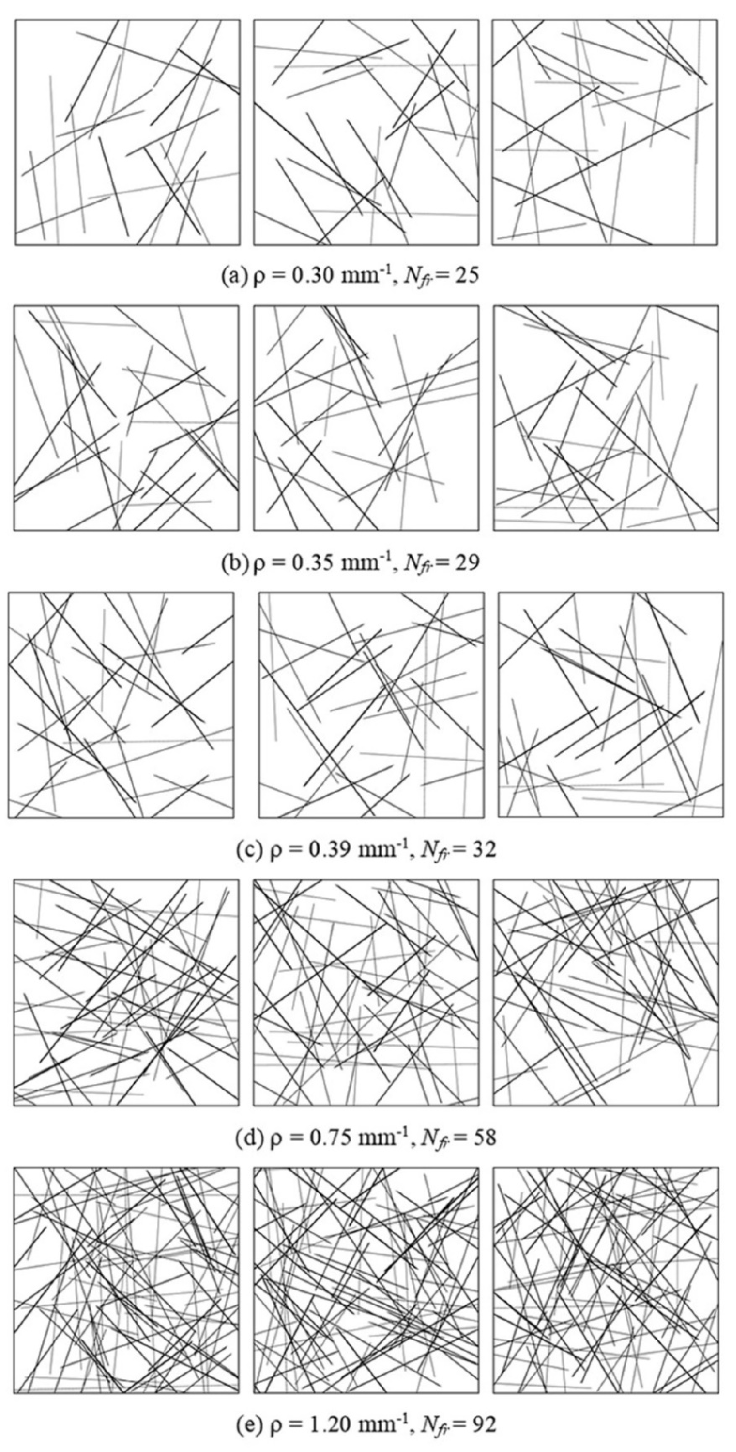
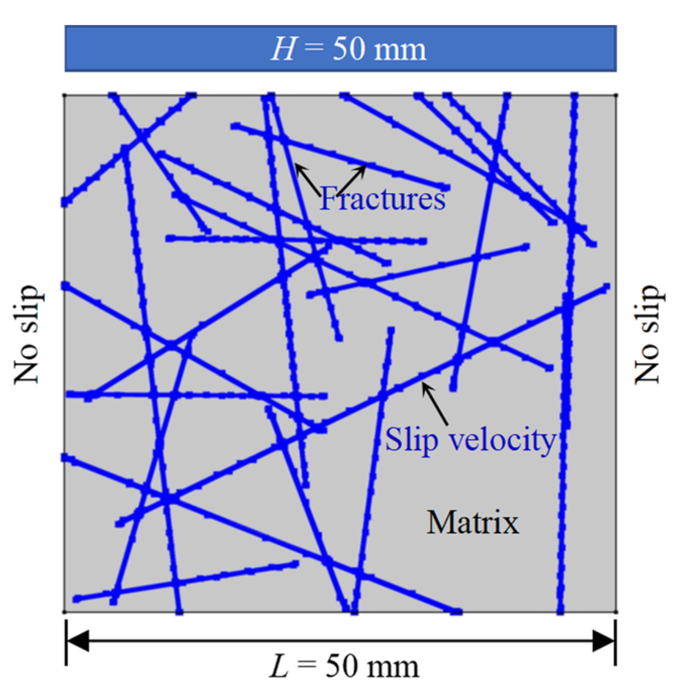
2.1. Fracture Network Generation

Fluid flow in fractured rocks refers to the fluid flow in both porous (matrix and micropores) and fractured media (fractures and faults). Microporous structures have low hydraulic conductivity and their permeability is directly related to porosity. The fracture permeability not only depends on the fracture density but is also determined by the fracture distribution characteristics (i.e., fracture length, fracture apertures, and azimuths). In this study, we built five series of fracture models with varying fracture densities and distributions. While this approach can be expanded for applications to real geological formations, we made the following assumptions to construct the fracture systems: (1) Each system is a two-dimensional (2-D) square domain with sides of length L. Fluid flows into the system from the top of the system. (2) Fractures are randomly positioned. (3) Fractures follow a power law distribution for length, a normal distribution for aperture, and a random distribution for orientation. (4) Only connected fractures are considered. The details of the approach used to generate the fracture models are discussed in the following section.

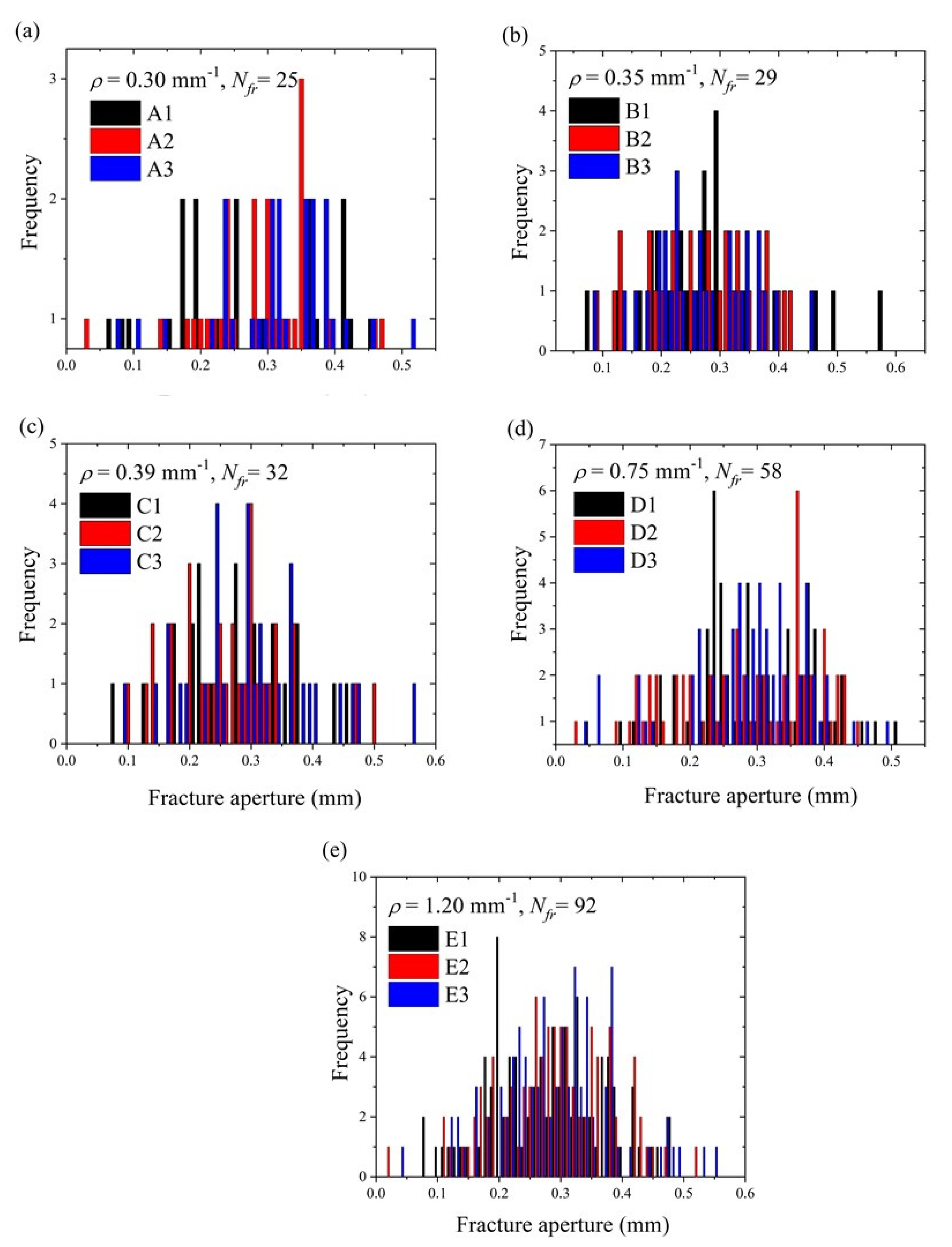
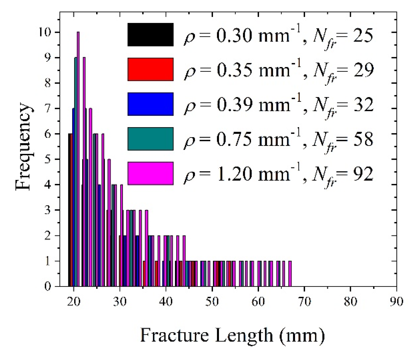
2.2. Fracture Length Distribution

The geometric parameters for real reservoir fractures generally have statistical rules and obey one or several types of probability distribution. Referring to the work by Zhang et al. [49], the power law distribution was used to characterize the fracture length in this study, which is the most widely used model to describe the fault length distribution of reservoir rocks [50,51,52,53,54]. The power law distribution of a fracture system is expressed as:

$$n\left(l\right)=\alpha l^{-a},$$

(1)

where n(l)dl refers to the fracture number that has a length interval [l, l+dl], $\alpha$ is a proportional coefficient that reflects the fracture density and depends on the fracture system size, and a is an exponent varying from one to three. The fracture density is defined as the cumulative fracture length per unit area in a fracture system, which can be can be calculated as [55]:

$$\mathsf{\rho }={\displaystyle \sum }nl/L^2,$$

(2)

where $\mathsf{\rho }$ means the fracture density (mm⁻¹), $n$ is the total number of fractures with a length of l in a fracture system, and L is the system size (mm).

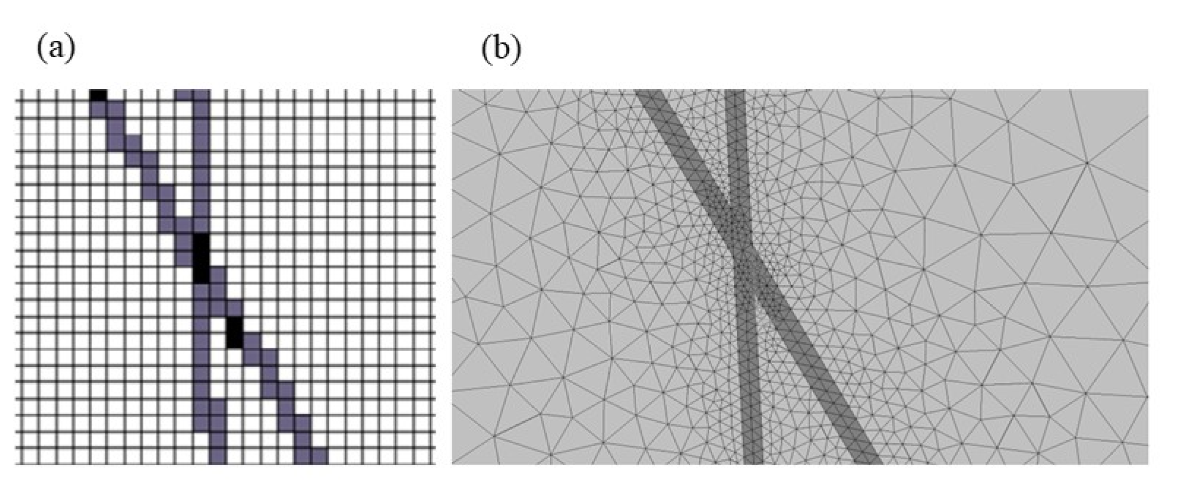
2.3. Determining Hydraulic Connections for a Given Fracture Network

The connectivity of individual fractures determines numerous fundamental properties for a fracture network to determine system connectivity. Compared with previous studies, we only needed to perform the network generation process once and the fracture density of the connected networks could be accurately controlled to generate fracture networks with varying connectivity. The connected networks not only satisfied geometric continuity but also conformed to the average degree of connectivity. Here, a percolation parameter, p, which is related to the fracture density, is used as the critical value below which the fracture system is not connected, whereas the fracture system is, on average, connected, i.e., we also consider that the matrix is permeable. For a 2D square fracture system (size L) with N fractures of constant length l, $p$ is calculated as:

$$p=N{l}^2/L^2$$

(3)

To generate a fracture network, we must determine three parameters to characterize the individual fracture geometry, i.e., the location, orientation, and length. The fracture center is randomly located in the system. The fracture orientation is also random, i.e., uniformly sampled from all directions. The fracture length (l) is sampled from its power law distribution. We use four geometry parameters to generate the fracture networks, i.e., the normalized system size, L_s = L/l_min; the normalized maximum length of the fracture, L_maxs = l_max/l_min (l_min and l_max refer to the minimum and maximum fracture lengths in a fracture system, respectively); the exponent a; and the ratio of r = a_s/a_sc. We refer to the fracture generation details reported by Zhang et al. [49]. For a given fracture system, the critical parameter, a_sc, is calculated and compared with the actual parameter, a_s. When a_s is much less than a_sc, i.e., r < 1, the system is viewed as non-connected. For systems with a_s near or above a_sc, i.e., r ≥ 1, the system is viewed as connected (the matrix is also considered to be permeable) and the steps described in the following section must be performed.

The fracture apertures in coal rock follow a normal distribution based on statistical data [9]. Based on their experiments, Wang et al. calculated the fracture apertures in coal rock, which ranged from 0.028 to 0.315 mm, with an average fractal aperture of 0.142 mm in a circular sectional area of 25 mm². Therefore, in this study, we used an average fractal aperture, W_av, of 0.284 mm for a square system with a size of L = 50 mm and a standard deviation of σ = 0.1 to generate the fracture networks. We controlled the fracture apertures between 0.03 and 0.63 mm. The fracture azimuths followed a random distribution, such that they were applicable to real geologic formations. The three fracture networks in each group had identical fracture densities.

Table 1. The initial geometric parameters of the fracture networks.

Model No.	r	lmax	lmin	Nfr	$\mathsf{\rho }$ (mm−1)	Fracture Aperture (mm)
						wav	σ	wmin	wmax
A1	1.1	55.29	20	25	0.30	0.284	0.1	0.07	0.57
A2								0.03	0.47
A3								0.07	0.51
B1	1.3	56.84		29	0.35			0.08	0.58
B2								0.09	0.42
B3								0.08	0.45
C1	1.5	58.89		32	0.39			0.08	0.46
C2								0.10	0.50
C3								0.09	0.56
D1	3.2	66.00		58	0.75			0.05	0.51
D2								0.03	0.47
D3								0.04	0.49
E1	5.1	67.3		92	1.20			0.08	0.48
E2								0.04	0.52
E3								0.04	0.55

lists the initial geometric parameters for the fracture networks. Figure 2 shows the fracture networks, while Figure 3 and Figure 4 show the fracture aperture and model length distributions with various fracture densities, respectively. These geometry parameters for the fracture networks correspond to real geological cases and lay a good foundation for experimental studies in the next step to improve the predictive capability of the numerical methods developed in this study.

2.4. Dual-Porosity Model for Gas Flow Simulation and Permeability ($\overline{\kappa }$) Calculations

Here, we developed a 2-D dual-porosity model to simulate the gas flow in fractured rocks. The model treats matrix and pore structures as one component and couples the flow in matrix pores and fractures to compute the equivalent permeability. To study the influences of pore–fracture structures on the permeability properties of fractured rocks, we used an identical fracture network with three rock rank matrix properties from mining areas to simulate gas flow and compute permeability. The three ranks of rocks from mining areas, i.e., I_rock, II _rock, and III_rock, were used to set the matrix properties. The properties of I_rock, II _rock, and III_rock for the matrix permeability, $k_m,$and porosity, ${\epsilon }_m$, were taken from the sandstone used in our experiments, coal [56], and oil reservoirs [57], respectively.

$$k_m=\{\begin{array}{c} 0.01 mD, {\mathrm{I}}_{\mathrm{rock}} \\ 6.46 mD, { \mathrm{II}}_{\mathrm{rock}}\\ 303.98 mD, {\mathrm{III}}_{\mathrm{rock}}\end{array},$$

(4)

$${\epsilon }_m=\{\begin{array}{c}0.04, {\mathrm{I}}_{\mathrm{rock}} \\ 0.1, { \mathrm{II}}_{\mathrm{rock}} \\ 0.25, {\mathrm{III}}_{\mathrm{rock},} \end{array}$$

(5)

Since fractures have much larger permeability than the matrices in tight reservoirs, solving such a nonlinear problem using traditional numerical methods poses difficulties. In this study, we divided the fractures and matrix into two domains to calculate the gas flow in a rock system. Variable exchanges between the velocity and pressure fields were used to simulate the coupling flows in the matrix and fractures. The compressible N–S equation was used to simulate methane flow in fractures [58] as follows:

$${\rho }_0\frac{\partial \mathit{u}}{\partial t}+{\rho }_0\left(\mathit{u}·\nabla \right)\mathit{u}=-\nabla \mathit{p}+\nabla ·\left(\mu \left(\nabla {u}+{\left(\nabla {u}\right)}^T\right)-\frac{2}{3}\mu \left(\nabla ·{u}\right)I\right),$$

(6)

$$\frac{\partial \rho }{\partial t}+\nabla ·\left(\rho \mathit{u}\right)=0$$

(7)

For the matrix, we used the compressible Brinkman equation, as follows:

$$0=-\nabla \mathit{p}+\nabla ·{\frac{\mu }{\epsilon }}_p\left(\nabla \mathit{u}+\nabla {\mathit{u}}^T\right)-\frac{2}{3}\mu {\frac{1}{\epsilon }}_p\left(\nabla ·\mathit{u}\right)-\frac{\mu }{k_m}\mathit{u},$$

(8)

$$\frac{\partial \rho }{\partial t}+\nabla ·\left(\rho \mathit{u}\right)=0,$$

(9)

where p is the pressure, u is the flow velocity, μ is the dynamic viscosity, ${\epsilon }_p$ is the porosity, and $k_m$ is the matrix permeability. The gas flows into the domain from the top of the system. The fluid velocity was initially zero and flow was driven by a hydraulic head between the bottom (y = 0) and top (y = L) of the system. The velocities at the grain boundaries equaled zero, i.e., “no slip” conditions.

We ensured that the flow was in a laminar regime by checking if the permeability remained constant. According to Darcy’s law, the absolute permeability of the fractured rocks was computed using the following equation:

$$k=\mu QL/\Delta \mathit{p}·A,$$

(10)

$$Q={{\displaystyle \int }}_s\mathit{v}·ds=\underset{n\to \infty }{\lim }{{\displaystyle \sum }}_{i=1}^n{\mathit{v}}_{\mathit{i}}{s}_i,$$

(11)

where$k$is the absolute permeability, Q is the total fluid flux, L is the system length, A is the cross-sectional area of flow (i.e., here we use the system size L), $\mathbf{\Delta }\mathit{p}$is the pressure difference at the inlets and outlets, respectively; ${\mathit{v}}_{\mathit{i}}$ and $s_i$ are the section velocity and section area at the outlets, respectively.

Due to Klinkenberg’s effects, gas permeability is usually greater than liquid permeability in tight reservoirs [59]. This is especially the case when the pressure difference is low, and therefore the rock permeability measured by gas is much larger than that measured by water [60]. In this study, the following corrected formula was used to calculate the equivalent gas permeability ${\overline{\kappa }}_g$, which considers Klinkenberg effects based on previous studies [60,61,62]:

$${\overline{\kappa }}_g=k\left[1+\left(b/{\mathit{p}}_{\mathit{a}\mathit{v}}\right)\right],$$

(12)

where $p_{av}$ represents the average gas pressure and b refers to the coefficient of Klinkenberg effects, which is modified using the following equation:

$$b=0.15\times k^{-0.37},$$

(13)

Figure 5 illustrates the domain settings and simulation boundary and

Table 2. Simulation model data.

Parameters	Value	Description
${\rho }_g$	0.67 kg/m3	Methane density
μ	1.1 × 10−5 (Pa·s)	Methane dynamic viscosity
H	50 mm	Hydraulic head

lists the model data used in this study. The fluid properties at normal temperature and pressure are used in the simulations.

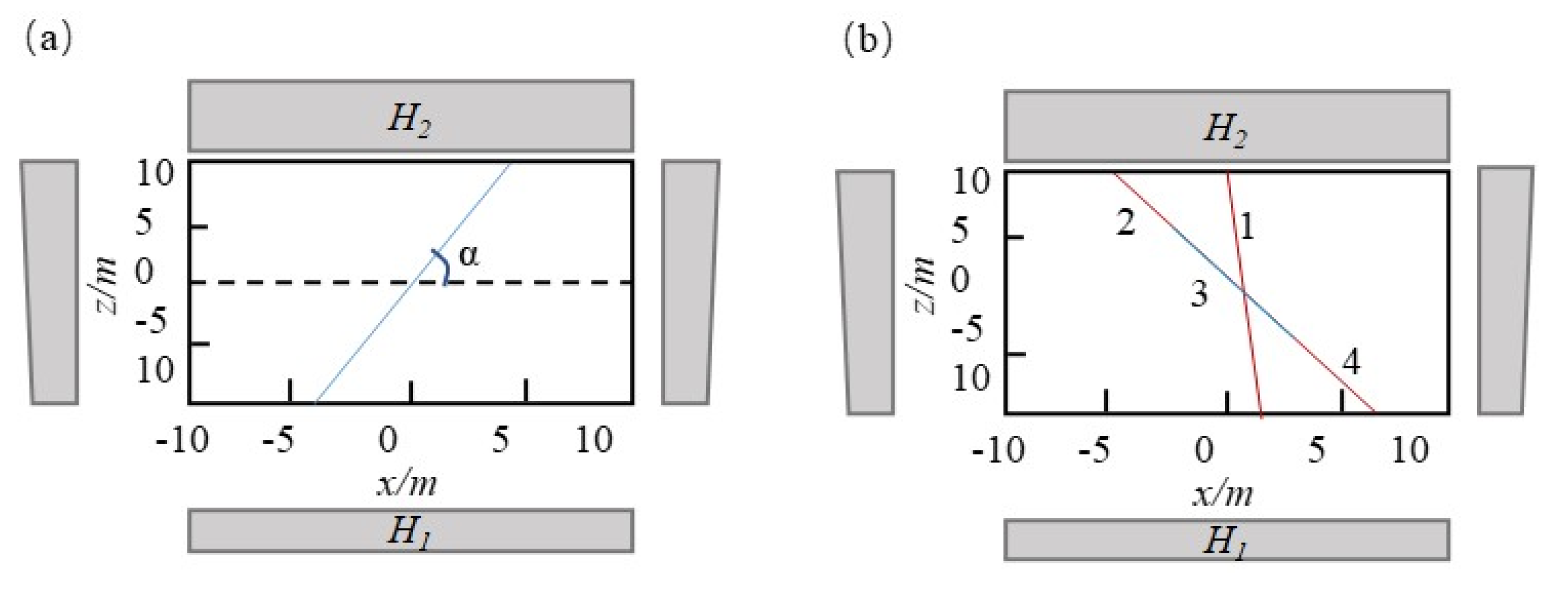
2.5. Dual-Porosity Model Verification

We performed flow simulations of a series of simple fracture networks to verify the accuracy of the dual-porosity model. We compared our numerical results with the theoretical solutions and numerical solutions from previous studies [63]. The previous studies assumed that the single fracture flow follows the cubic law and used the flow-equivalent principle to calculate the equivalent fracture permeability [64], which is expressed with the following equation:

$$k_{feq}=l_e{}^3\left(\gamma w\right),$$

(14)

where $l_e$is the element length of a square, w is the fracture aperture, and $\gamma$ is the coefficient related to the roughness of the fracture surface, i.e., when the fracture is straight and smooth $\gamma$= 1/12, otherwise $\gamma$ < 1/12. This formula reflects the effects that the fracture aperture, fracture surface roughness, and numerical method (element size) have on the equivalent permeability of the fractures.

The verification fracture system uses an identical fracture structure to that reported in [63] to compare the numerical results with their numerical solutions. The domain is a square (20 m × 20 m), as shown in Figure 6a. For a single fracture network, we set nine sets of single fractures with different slopes ranging from 50° to 90°, with an interval of 5°. A single fracture passes through the coordinate (0, 0) and the fracture aperture is equal to 5 mm.

A hydraulic head (H₁ = 30 m at the top and H₂ = 10 m at the bottom) drives the flow, with a vertical hydraulic gradient of 1 m/m at the left and right boundaries of the fracture system (Figure 6). To compare our results with numerical solutions from [63], we initialized the matrix with a minimum permeability of 1.0 × 10⁻²⁰ m² and a porosity of 1.0 × 10⁻¹⁰ to ensure that flow only occurred in the fractures. The theoretical solution of downstream outlet flow through a single fracture is given by the following equation:

$${\mathit{q}}_{\mathit{a}}={\mathsf{\rho }}_w\mathit{g}{l}_e{}^3/\left(\gamma \mu \right)\left(H_2-H_1\right)/l_f,$$

(15)

where ${\rho }_w$ is the water density (i.e., ${\rho }_w$ = 998.4 kg/m³), $\mathit{g}$ is the gravitational acceleration (i.e., $\mathit{g}$ = 10 m/s², $\mu$ is equal to 1.005 × 10⁻³ Pa·s. We also assume that the fracture surface is smooth, with a value for $\gamma$ of 1/12.

Table 3. Comparison of the simulation results for different simple fracture networks with analytical solutions.

Fracture Azimuth (º)	${\mathit{q}}_{\mathit{a}}({\mathbf{m}}^2/\mathbf{s})$
	Analytical Solutions	Numerical Simulation	Deviation (%)
50	0.0793	0.0826	4.16
55	0.0848	0.0848	0.00
60	0.0896	0.0882	−1.56
65	0.0938	0.0928	−1.07
70	0.0972	0.0937	−3.60
75	0.0999	0.0997	−0.20
80	0.1019	0.1002	−1.67
85	0.1031	0.1008	−2.23
90	0.1035	0.1010	−2.42

lists the simulation results.

Table 4. Parameters for the intersecting fractures and downstream outlet flow rate.

No.	Endpoint Coordinates (x, y)	Endpoint Coordinates (x, y)	Fracture Aperture (m)	${\mathit{q}}_{\mathit{a}}({\mathbf{m}}^2/\mathbf{s})$
				Analytical Solutions	Numerical Simulation
1	(0.7500, −10.0)	(−0.2500, 10.0)	0.004	0.1426	0.1417
2	(−2.8750, 5.0)	(−5.7500, 10.0)	0.005
3	(1.4375, −2.5)	(−2.8750, 5.0)	0.005
4	(5.7500, −10.0)	(1.4375, −2.5)	0.005

lists a comparison of our numerical results for nine single fractures with different dip angles with the analytical solutions. Our model’s numerical solutions are slightly smaller than the theoretical solutions, whereby the deviation fluctuates within 5%.

Table 5. Comparison of the simulation results for different simple fracture networks with numerical solutions from the MEPM [63].

Fracture Azimuth (º)	${\mathit{q}}_{\mathit{a}} ({\mathbf{m}}^2/\mathbf{s})$
	MEPM Solutions	Numerical Simulation	Deviation (%)
50	0.0811	0.0826	1.85
55	0.0868	0.0848	−2.30
60	0.0919	0.0882	−4.03
65	0.0964	0.0928	−3.73
70	0.1000	0.0937	−6.30
75	0.0984	0.0997	1.32
80	0.1002	0.1002	0.00
85	0.1011	0.1008	−0.30
90	0.1040	0.1010	−2.88

provides a comparison of our numerical results with the corresponding results from the study by Wang et al. [63] and indicates that our calculation results are slightly smaller than the corresponding results reported in the latter, whereby deviations fluctuate within 6.5%. This is because different from the quadrilateral mesh used in the modified equivalent permeability model (MEPM) of Wang et al. [63], our model uses a free triangle mesh. The fracture and matrix were divided into two domains for meshing and the fracture area was meshed with a size ratio of fracture apertures to mesh elements that was larger than 0.5 [65] (see Figure 7). This type of meshing can ensure that each fracture is accurately characterized by the fractured mesh, such that the actual flow paths are very close to the fracture length. Although the meshing accuracy is directly related to the actual flow paths, results with different mesh accuracies all fluctuate around the theoretical solution, which indicates the accuracy of the proposed dual-porosity model.

Figure 6b shows the intersecting fracture network. There are 4 cracks, namely through fracture 1 and non-through fractures 2, 3, and 4, however fractures 2, 3, and 4 are connected and form a hydraulic conduit. When calculating the theoretical fracture flow solution, the downstream flow flux is the total flow in two single through fractures. The model parameter settings and boundary conditions are identical to those used in single fracture studies. Table 4 shows the intersecting fracture parameters and downstream outlet flow flux. The results demonstrate that the downstream outlet flow (0.1417 m²/s) is quite similar to the MPEM numerical solution (0.1424 m²/s) from the study by Wang et al. [63], as well as the theoretical solution (0.1426 m²/s). Our model can also achieve good simulation results for intersecting fractures and non-through fractures, verifying the validity of the dual-porosity model.

3. Results and Discussions

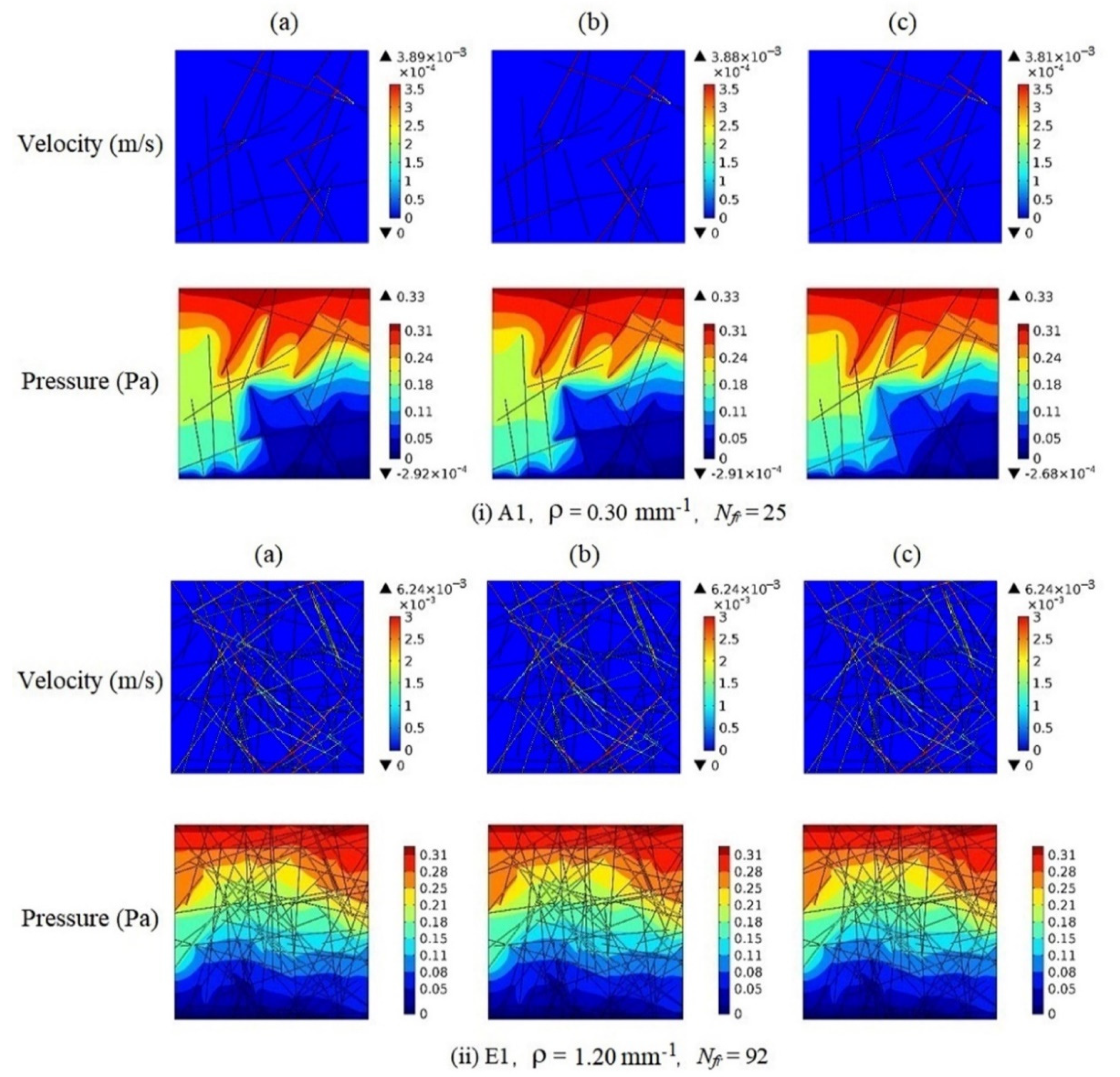
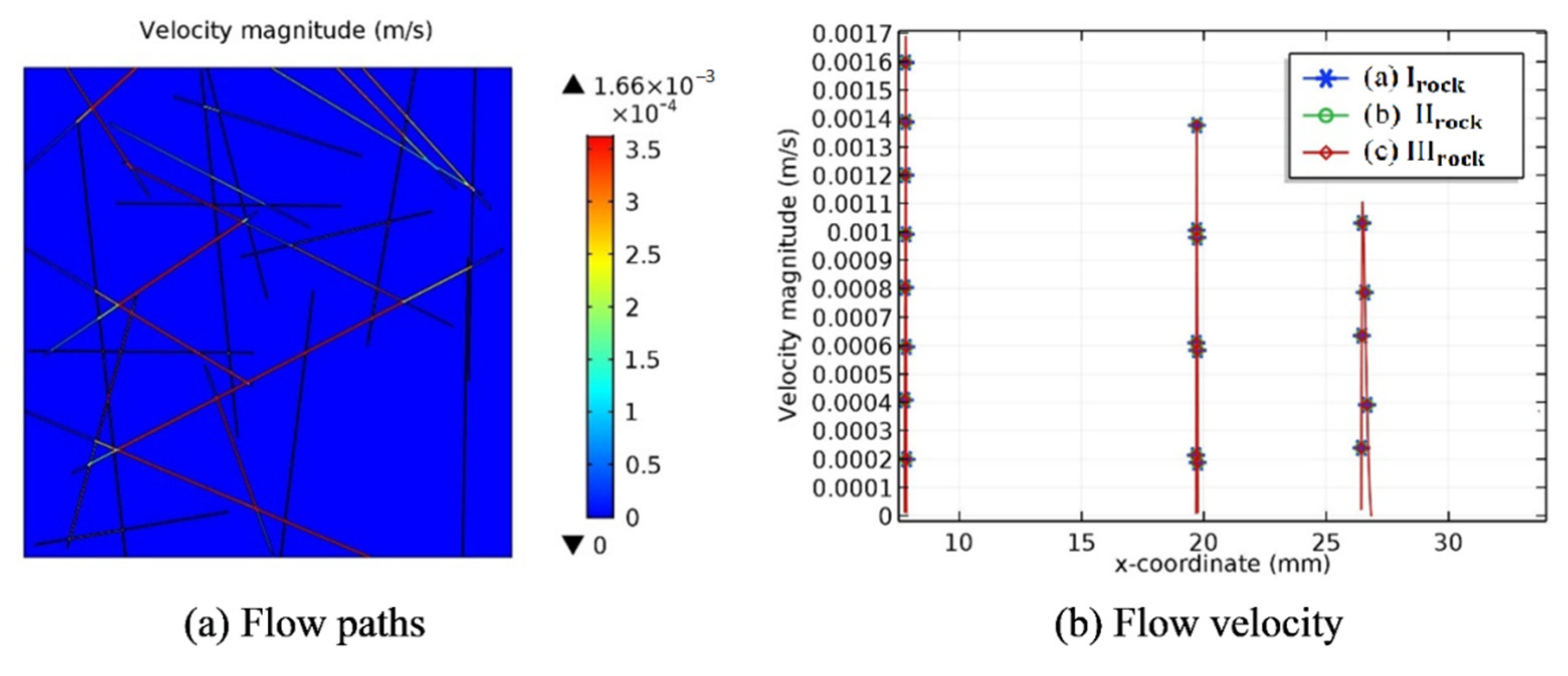
3.1. Flow Velocity and Pressure Profile

Figure 8 demonstrates the COMSOL^© Multiphysics results predicted using the methane velocity and pressure distribution values of the three rocks with fracture densities of 0.30/mm and 1.20/mm. We observed that as the fracture density increased, the fracture connectivity improved, the main flow paths increased, and the flow velocity gradually increased. The maximum flow velocity in the A1 model was 3.89 mm/s, while the flow velocity in the E model increased to 6.24 mm/s, i.e., 0.65-fold. The fracture number increased 3-fold and the main flow paths also significantly increased. The flow had clear hydraulic paths, which consisted of several connected fracture clusters. Less or even flow did not occur in the majority of connected fractures.

The fracture permeability values were much larger than the matrix permeability values, i.e., 10⁴–10⁹-fold larger (see the velocity at the bottom of models A1 and E1 in Figure 9). For the low-density fracture model A1, the gas flow velocity and pressure gradient changed slightly with increasing matrix permeability. For the high-density fracture model E1, there were no significant changes in the gas flow velocity or pressure gradient. The matrix flow velocity of III_rock increased, i.e., approximately 10³–10⁶-fold larger than that of I_rock and II_rock. The low fracture density model A1 had a small number of fracture outlets at the bottom and the matrix contribution to the rock permeability was relatively large. In contrast, the high fracture density model E1 had a large number of fracture outlets at the bottom and the matrix made nearly no contribution to rock permeability relative to fracture flow. We suggest that for rocks with low fracture densities, the matrix will significantly contribute to rock permeability. These results indicate that the proposed dual-porosity model is capable of quantitatively and visually predicting the flow velocity paths and the pressure distribution of tight fracture rocks.

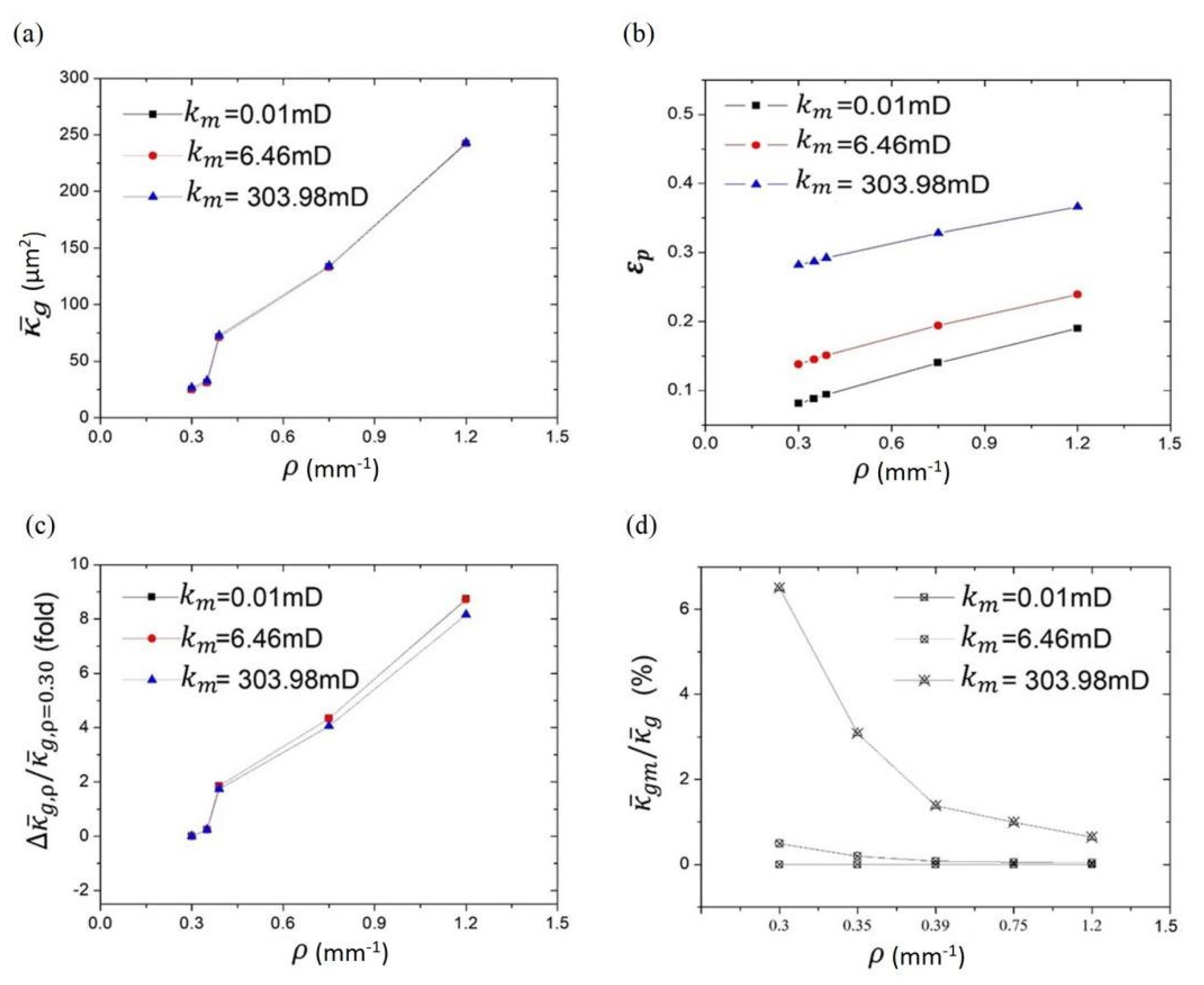
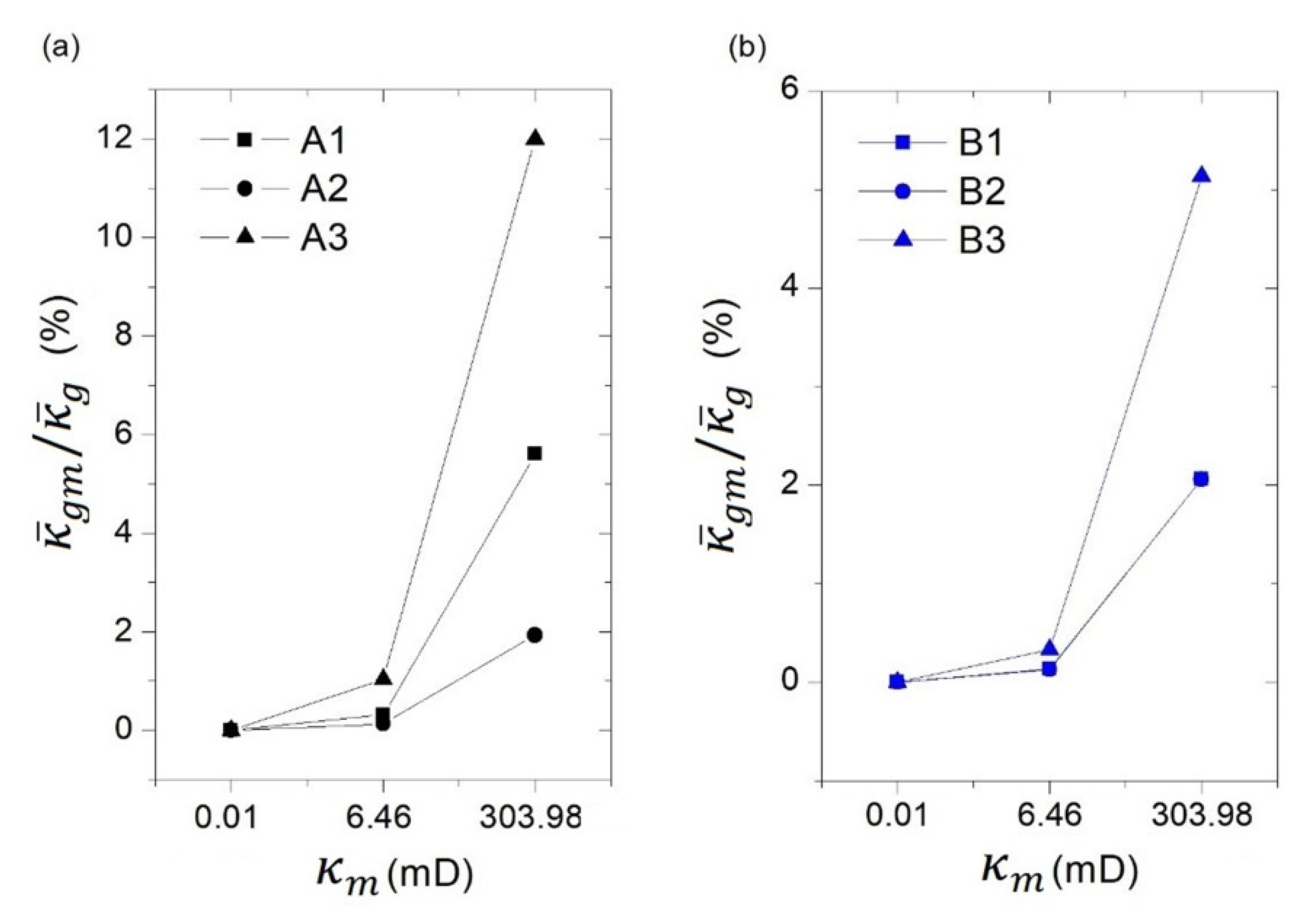
3.2. Estimation of Fractured Rock Permeability

Based on a qualitative analysis, flow paths increase with the fracture number, and rock permeability increases as the fracture density becomes larger.

Table 6. Equivalent permeability and total porosity of rocks with three different matrix properties.

Fracture Density ρ (mm−1)	Equivalent Gas Permeability ${\overline{\mathit{\kappa }}}_{\mathit{g}}\left(\mathsf{\mu }{\mathbf{m}}^2\right)$			Total Porosity εp
	Irock	II rock	IIIrock	Irock	II rock	IIIrock
0.30	24.91	24.96	26.53	0.081	0.138	0.282
0.35	30.96	31.00	32.65	0.088	0.145	0.287
0.39	71.13	71.17	72.75	0.094	0.151	0.292
0.75	133.01	133.03	134.08	0.140	0.194	0.328
1.20	242.35	242.6	242.97	0.190	0.239	0.366

lists the simulation results for the equivalent permeability and total porosity.

Figure 10a,b plot the variations in equivalent permeability and total porosity with the fracture density and different rock rank types, respectively. Here, the total porosity refers to the total volume fraction of pores and fractures in the fracture system. The permeability and porosity of fractured rocks increased with increases in the fracture density, $\rho$, which was consistent with field examples [66]. Based on Figure 10c, one can observe that the permeability of the three rock ranks has the same variation trend as with an increase in fracture density. Elevated fracture densities result in larger increases in the equivalent permeability with the growth of the fracture density. With a fracture density $\rho$ of 0.30/mm, the fracture density increases by 16.7% and the equivalent permeability increases by approximately 24.3%. The fracture density increases by 3-fold at a $\rho$ of 1.2 (mm⁻¹) and the equivalent permeability increases by approximately 8.73-fold.

At the same time, we can observe that the equivalent permeability of fractured rocks varies little with increases in the porosity and matrix permeability relative to the influences of the fracture density, which is consistent with field examples [66]. However, for low-density fracture networks, our results indicate that there is a considerable change in the equivalent permeability due to matrix properties. Figure 10d compares the matrix contribution ratios of flow with various fracture densities. For I_rock and II_rock, there is a very small matrix contribution, which is near zero, but the matrix contribution from III_rock can reach nearly 6.5% of the total flow. As the fracture density increases, the permeability, which first increases, then gradually decreases with the matrix permeability. When the fracture density was 1.2/mm, the matrix contribution to rock permeability was nearly zero. Our results also indicate that the matrix contribution in model A3 can reach 11.98% (see Figure 11). This is mainly due to the fact that despite the good fracture connectivity, there are both fewer main flow paths and fractures at the bottom boundary (see Figure 12), which ultimately led to a weakened fracture flow and a relative increase in the matrix contribution to the equivalent permeability. The matrix velocity (10⁻³ m/s) of III_rock was 3–5 orders of magnitude larger than that of I_rock (10⁻¹² m/s) and II_rock (10⁻⁹ m/s). Additionally, the matrix contribution to the total flow, despite being approximately 4 orders of magnitude less than the fracture flow velocity (10⁻³ m/s), was relatively significant. Therefore, we can conclude that when the fracture/matrix permeability ratio, i.e., k_f/k_m, is less than or equal to 10⁴ for low fracture density rocks (i.e., $\rho$≤ 0.35 (mm⁻¹), w_av ≤ 0.284 mm), the matrix can contribute significantly to the total flow. Here, fracture permeability refers to the permeability of a single fracture and is calculated as $k_f=w^2/12$, where w is the single fracture aperture.

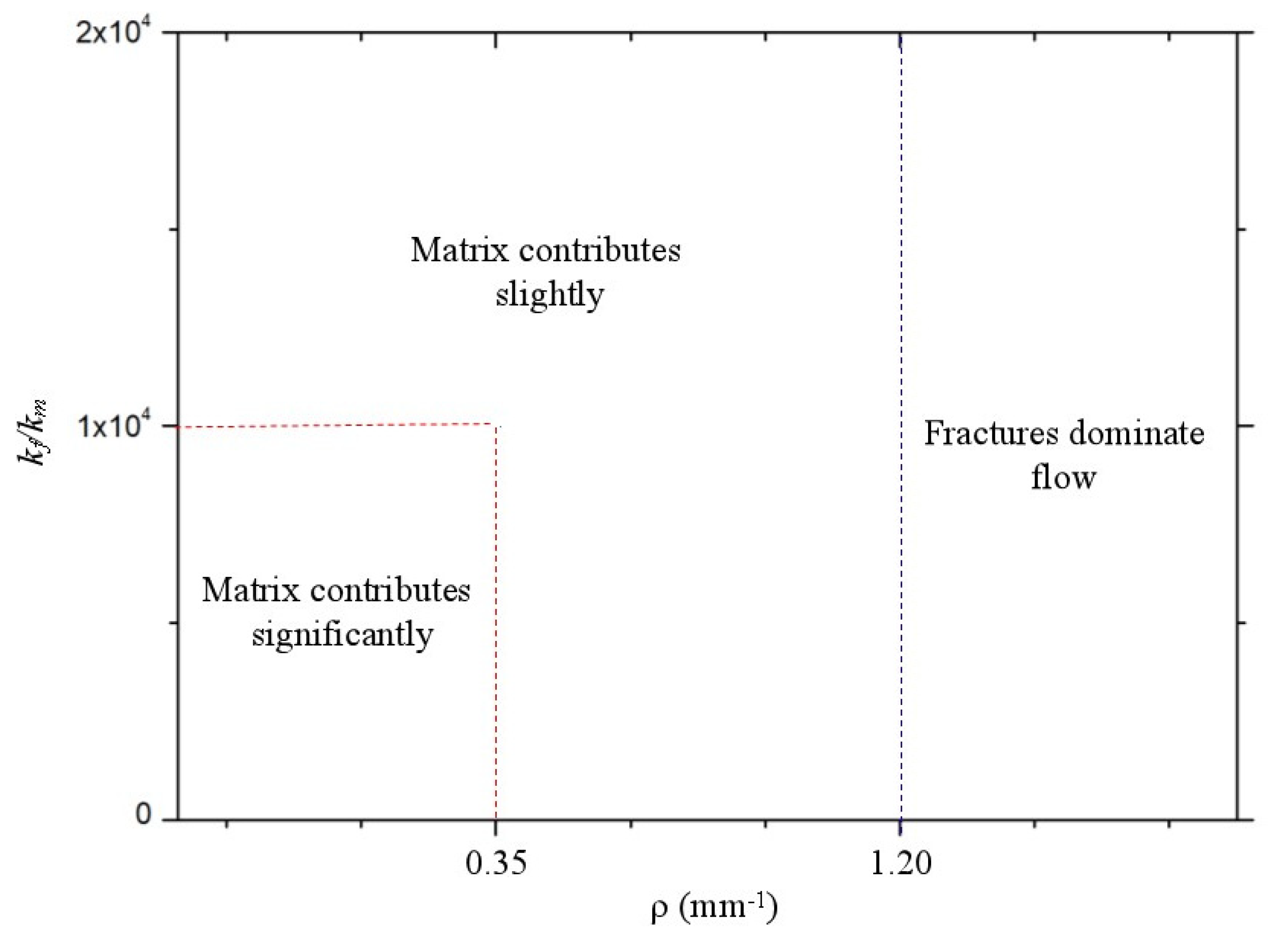
3.3. The Quantitative Relationship between Pore–Fracture Distribution and Permeability

To better understand the impacts that coupled flow in a matrix and fractures has on rock permeability, we calculated the variations in permeability regarding the fracture density and matrix permeability to quantitatively analyze the permeability of fractured rocks. We found that the equivalent permeability ${\overline{\kappa }}_g$of fractured rocks obeys the linear exponential function of the fracture density, $\mathsf{\rho }$, and matrix permeability, $k_m$, which is shown in the following equation:

$${\overline{\kappa }}_g=-109.83+106.69ex{p}^{\mathsf{\rho }}+3.71ex{p}^{k_m}; R^2=0.97$$

(16)

Figure 13 illustrates the 3-D relationship between permeability,${\overline{\kappa }}_g$ (µm²), fracture density, $\rho$ (mm⁻¹), and matrix permeability, k_m (µm²). According to this relationship, for a given fractured rock structure, the permeability can be estimated by the statistical distribution characteristics of the fractures and matrix. This relationship provides data references when evaluating fracturing effects.

Since the contribution of the matrix flow to the total flow is weaker than that of the fracture structures, we observed that the permeability increases with matrix permeability. However, using Equation (16), we speculated that the matrix contribution to the total flow increases with a decrease in the fracture density. When the fracture density, $\rho$, is less than or equal to 0.30 and the ratio of the fracture–matrix permeability, k_f/k_m, is less than or equal to 10⁴ for the fracture system developed in this study (w_av = 0.284 mm for the random fracture orientation, while the matrix permeability is between 0.01 and 1000 mD), the matrix contribution to the rock permeability can be significant. In contrast, when the fracture density, ρ, is greater than or equal to 1.2, the matrix contribution is nearly negligible.

Fluid flow partitioning between the matrix and fractures in fractured rocks is proposed in Figure 14. Compared with the study by Matthäi et al. [31], a two-dimensional partitioning of fracture–matrix flow concerning the fracture heterogeneity and the fracture–matrix permeability ratios (k_f/k_m) was established for characteristic flow regimes. This indicated that critical behavior exists when the flow is either dominated by the matrix or fractures. Similar to the results of Matthäi et al. [31], a critical behavior was observed around k_f/k_m ≈ 10⁴. For matrix permeability of 0.01 mD ≤ k_f ≤ 1000 mD and a ratio of fracture–matrix permeability of k_f/k_m ≤ 10⁴, the critical behavior occurs near $\rho$ = 0.35 mm⁻¹ (w_av = 0.284 mm). However, when the fracture density reaches a critical value, the flow is mainly dominated by fracture flow. This consists of three zones: (i) when the fracture density is extremely low (ρ ≤ 0.35 mm⁻¹, w_av ≤ 0.284 mm), the matrix contributes significantly to the total flow; (ii) when the fracture density is low or medium, the matrix slightly affects the total flow; (iii) when the fracture density is sufficiently high ($\rho$ ≥ 1.2 mm⁻¹, w_av ≤ 0.284 mm), fracture flow completely dominates the total flow.

4. Conclusions

In this study, we developed a dual-porosity model to investigate the permeability of tight fractured rocks, with a special focus on the quantitative analysis of the coupling contributions of fractures and micropores to the equivalent permeability of fractured reservoirs using variable exchanges between the velocity and pressure fields. Percolation theory was used to establish fracture networks with complicated fracture heterogeneity via self-developed codes, characterized by fracture density and percolation possibility. The rock permeability calculations considered gas compressibility and Klinkenberg effects. The two-dimensional partitioning schemes for three flow regimes were proposed to further demonstrate the fracture–matrix flow partitioning in fractured reservoirs with various fracture densities and fracture/matrix permeability ratios. The main results of this study are as follows:

(i) As the fracture density increases, the fracture connectivity gradually improves. The gas permeability significantly increases with an increase in the fracture density, which is due to increases in the fluid velocity and flow paths;

(ii) The gas flow in fractured rocks has clear hydraulic paths, which consist of several connected fracture clusters. Lower or even flow did not occur in the majority of the connected fractures;

(iii) Three flow regions were divided to demonstrate fracture–matrix flow using the two-dimensional partitioning method. The contribution of fractures and matrix micropores toward gas permeability can be determined using the fracture/matrix permeability ratios and the fracture density. The contribution of matrix micropores cannot be neglected if the fracture density is lower than a critical value;

(iv) We derived the quantitative relationships between the fracture density, porosity, and equivalent permeability for the three ranks of rocks. Permeability is characterized by exponential growth with increases in fracture density and rock porosity. This study intends to provide a research basis and numerical reference for the quantitative analysis and visual description of the relationships between rock permeability and pore–fracture structures.

It is noteworthy that although we were able to validate the dual-porosity model based on the tests of a series of single-fracture and cross-fracture models, there is still a lack of direct experimental verification of the proposed dual-porosity model. To overcome this, we intend to used three-dimensional printing (or additive manufacturing) technology [67] to fabricate a transparent dual-porosity model for future experimental investigations and to improve the predictive capability of the current numerical model. Moreover, because of the extremely high heterogeneity and anisotropy of the fracture structures in the real rocks, more factors need to be considered to better characterize the real rock structures and describe the 3D flow behavior in future studies and to explore the controlling mechanism of rock permeability in a dual-porosity model with micropores and fractures. Considering the primary purpose of this study and the limited length of research articles, we will discuss this issue in our follow-up studies.

References

1. Chen, X.L.; Tang, X.M.; Qian, Y.P. Propagation characteristics of multipole acoustic logging in cracked porous tight formations. Chin. J. Geophys. 2014, 57, 2961–2970. [Google Scholar]
2. Zhi, Z.W.; Cheng, W.Z.; Jun, W.H.; Jin, C.M. Research Advances and Exploration Significance of Large-area Accumulation of Low and Medium Abundance Lithologic Reservoirs. Acta Geol. Sin. 2008, 82, 463–476. [Google Scholar]
3. Fu, P.; Johnson, S.M.; Carrigan, C.R. An explicitly coupled hydro-geomechanical model for simulating hydraulic fracturing in arbitrary discrete fracture networks. Int. J. Numer. Anal. Met. 2014, 37, 2278–2300. [Google Scholar] [CrossRef]
4. Hu, X.; Xie, J.; Cai, W.; Wang, R.; Davarpanah, A. Thermodynamic effects of cycling carbon dioxide injectivity in shale reservoirs. J. Petrol. Sci. Eng. 2020, 195, 107717. [Google Scholar] [CrossRef]
5. Teimoori, A.; Chen, Z.; Rahman, S.S.; Tran, T. Effective Permeability Calculation Using Boundary Element Method in Naturally Fractured Reservoirs. Liq. Fuels Technol. 2005, 23, 693–709. [Google Scholar] [CrossRef]
6. Abdelazim, R.; Rahman, S.S. Estimation of Permeability of Naturally Fractured Reservoirs by Pressure Transient Analysis: An Innovative Reservoir Characterisation and Flow Simulation. J. Petrol. Sci. Eng. 2016, 145, 404–422. [Google Scholar] [CrossRef]
7. Park, Y.C.; Sung, W.M.; Kim, S.J. Development of a FEM Reservoir Model Equipped with an Effective Permeability Tensor and its Application to Naturally Fractured Reservoirs. Energy Sources 2002, 24, 531–542. [Google Scholar] [CrossRef]
8. Gang, T.; Kelkar, M.G. Efficient History Matching in Naturally Fractured Reservoirs. In Proceedings of the SPE/DOE Symposium on Improved Oil Recovery, Tulsa, OK, USA, 22–26 April 2006. [Google Scholar]
9. Wang, C.; Zhai, P.; Wang, L.; Wang, C.; Zhang, X.; Wu, X.; Jiang, Y. Careful features of lithotype cracks based on Micro-CT technology. Coal Sci. Technol. 2017, 45, 137–142. [Google Scholar] [CrossRef]
10. Peng, P.; Ju, Y.; Wang, Y.; Wang, S.; Gao, F. Numerical analysis of the effect of natural microcracks on the supercritical CO2 fracturing crack network of shale rock based on bonded particle models. Int. J. Numer. Anal. Met. 2017, 41, 1–23. [Google Scholar] [CrossRef]
11. Cheng, H.; Ju, Y.; Xu, T.; Yue, S.; Jia, T.; Neupane, B.; Han, K.; Yu, Q.; Zhu, H.; Cai, J. Full-Scale and Multi-Method Combined Characterization of Micro/Nano Pores in Organic Shale. J. Nanosci. Nanotechnol. 2017, 17, 6634–6644. [Google Scholar]
12. Hu, Q.; Zhang, Y.; Meng, X.; Li, Z.; Xie, Z.; Li, M. Characterization of micro-nano pore networks in shale oil reservoirs of Paleogene Shahejie Formation in Dongying Sag of Bohai Bay Basin, East China. Petrol. Explor. Dev. 2017, 44, 720–730. (In Chinese) [Google Scholar] [CrossRef]
13. Chen, M.; Bai, M.; Roegiers, J.C. Permeability Tensors of Anisotropic Fracture Networks. Math. Geol. 1999, 31, 335–373. [Google Scholar] [CrossRef]
14. Min, K.B.; Jing, L.; Stephansson, O. Determining the equivalent permeability tensor for fractured rock masses using a stochastic REV approach: Method and application to the field data from Sellafield, UK. Hydrogeol. J. 2004, 12, 497–510. [Google Scholar] [CrossRef]
15. Snow, D.T. Anisotropie Permeability of Fractured Media. Water Resour. Res. 1969, 5, 1273–1289. [Google Scholar] [CrossRef]
16. Wanniarachchi, W.A.M.; Ranjith, P.G.; Perera, M.S.A.; Rathnaweera, T.D.; Zhang, D.C.; Zhang, C. Investigation of effects of fracturing fluid on hydraulic fracturing and fracture permeability of reservoir rocks: An experimental study using water and foam fracturing. Eng. Fract. Mech. 2018, 194, S001379441731353X. [Google Scholar] [CrossRef]
17. Uehara, S.; Takahashi, M.; Oikawa, Y.; Masuda, K. Depth dependency of fracture permeability in Neogene mudstone. Agu Fall Meet. Abstr. 2009, 2009, H13E-1023. [Google Scholar]
18. Liang, Y.; Tsuji, S.; Jia, J.; Tsuji, T.; Matsuoka, T. Modeling CO2–Water–Mineral Wettability and Mineralization for Carbon Geosequestration. Acc. Chem. Res. 2017, 50, 1530–1540. [Google Scholar] [CrossRef]
19. Zhong, Y.; Zhang, H.; Shao, Z.; Li, K. Gas Transport Mechanisms in Micro- and Nano-Scale Matrix Pores in Shale Gas Reservoirs. Chem. Technol. Fuels Oil 2015, 51, 545–555. [Google Scholar] [CrossRef]
20. Duan, Y.; Cao, T.; Yang, X.; Zhang, Y.; Wu, G. Simulation of gas flow in nano-scale pores of shale gas deposits. J. Southwest Petrol. Univ. 2015, 37, 63–68. [Google Scholar]
21. Davarpanah, A.; Mirshekari, B. Experimental Investigation and Mathematical Modeling of Gas Diffusivity by Carbon Dioxide and Methane Kinetic Adsorption. Ind. Eng. Chem. Res. 2019, 58, 12392–12400. [Google Scholar] [CrossRef]
22. Rasmussen, T.C.; Jim-Yeh, T.C.; Evans, D.D. Effect of variable Fracture Permeability/Matrix Permeability Ratios on Three-Dimensional Fractured Rock Hydraulic Conductivity. 1989. pp. 337–358. Available online: https://eurekamag.com/research/018/362/018362917.php (accessed on 23 March 2021).
23. Lough, M.F.; Lee, S.H.; Kamath, J. An Efficient Boundary Integral Formulation for Flow Through Fractured Porous Media. J. Comput. Phys. 1998, 143, 462–483. [Google Scholar] [CrossRef]
24. Lee, S.H.; Lough, M.F.; Jensen, C.L. Hierarchical modeling of flow in naturally fractured formations with multiple length scales. Water Resour. Res. 2001, 37, 443–455. [Google Scholar] [CrossRef]
25. Neuman, S.P. Multiscale Relationships Between Fracture Length, Aperture, Density and Permeability. Geophys Res. Lett. 2015, 35, 1092–1104. [Google Scholar] [CrossRef]
26. Bai, M.; Ma, Q.; Roegiers, J.C. Dual-porosity behaviour of naturally fractured reservoirs. Int. J. Numer. Anal. Met. 2010, 18, 359–376. [Google Scholar] [CrossRef]
27. Cai, L.; Ding, D.Y.; Wang, C.; Wu, Y.S. Accurate and Efficient Simulation of Fracture–Matrix Interaction in Shale Gas Reservoirs. Transp. Porous Med. 2015, 107, 305–320. [Google Scholar] [CrossRef]
28. Wang, W.; Wei, Y.; Hu, X.; Hua, L.; Wu, B. A Semi-analytical Model for Simulating Real Gas Transport in Nanopores and Complex Fractures of Shale Gas Reservoirs. AIChE J. 2017, 64, 326–337. [Google Scholar] [CrossRef]
29. Abbasi, M.; Madani, M.; Sharifi, M.; Kazemi, A. Fluid flow in fractured reservoirs: Exact analytical solution for transient dual porosity model with variable rock matrix block size. J. Petrol. Sci. Eng. 2018, 164, 571–583. [Google Scholar] [CrossRef]
30. Rahman, M.M.; Rahman, S.S. Studies of Hydraulic Fracture-Propagation Behavior in Presence of Natural Fractures: Fully Coupled Fractured-Reservoir Modeling in Poroelastic Environments. Int. J. Geomech. 2013, 13, 809–826. [Google Scholar] [CrossRef]
31. Matthäi, S.K.; Belayneh, M. Fluid flow partitioning between fractures and a permeable rock matrix. Geophys Res. Lett. 2004, 31, 7. [Google Scholar] [CrossRef]
32. Sanaee, R.; Oluyemi, G.F.; Hossain, M.; Oyeneyin, M.B. Fracture-Matrix Flow Partitioning and Cross Flow: Numerical Modeling of Laboratory Fractured Core Flood. In Proceedings of the 2012 COMSOL Conference, Milan, Italy, 10–12 October 2012. [Google Scholar]
33. Lei, Q.; Wang, X.; Min, K.-B.; Rutqvist, J. Interactive roles of geometrical distribution and geomechanical deformation of fracture networks in fluid flow through fractured geological media. J. Rock Mech. Geotech. Eng. 2020, 12, 780–792. [Google Scholar] [CrossRef]
34. Wong, D.L.Y.; Doster, F.; Geiger, S.; Kamp, A. Partitioning Thresholds in Hybrid Implicit-Explicit Representations of Naturally Fractured Reservoirs. Water Resour. Res. 2020, 56, e2019WR025774. [Google Scholar] [CrossRef]
35. Jia, C. Characteristics of a Superimposed Basin and the Promise of a Buried Petroleum Play. In Characteristics of Chinese Petroleum Geology; Springer: Berlin/Heidelberg, Germany, 2012. [Google Scholar]
36. Karpyn, Z.T.; Alajmi, A.; Radaelli, F.; Halleck, P.M.; Grader, A.S. X-ray CT and hydraulic evidence for a relationship between fracture conductivity and adjacent matrix porosity. Eng. Geol. 2009, 103, 139–145. [Google Scholar] [CrossRef]
37. Liu, J.; Jiang, Y.; Zhao, Y. Progress in the Application of AE and CT in Research of Coal and Rock Fracture Propagation. Met. Mine 2008, 5, 63–66. [Google Scholar]
38. Kock, T.D.; Boone, M.A.; Schryver, T.D.; Stappen, J.V.; Derluyn, H.; Masschaele, B.; Schutter, G.D.; Cnudde, V. A Pore-Scale Study of Fracture Dynamics in Rock Using X-ray Micro-CT Under Ambient Freeze–Thaw Cycling. Environ. Sci. Technol. 2015, 49, 2867–2874. [Google Scholar] [CrossRef] [PubMed]
39. Ya, L.I.; Jie, Y.U.; Man, X.U.; Hui, W.U. SEM Study on Fracture Characteristic of Mineralized wall Rock Samples of Nannigou Gold Deposit in Guizhou under High Temperature and High Pressure. Bull. Miner. Petrol. Geochem. 2000, 39, 5271–5276. [Google Scholar]
40. Neupane, B.; Ju, Y.; Huang, C. Micro/Nano-Pore Structure Characterization of Western and Central Nepal Coals Using Scanning Electron Microscopy and Gas Adsorption. J. Nanosci. Nanotechnol. 2017, 17, 1–7. [Google Scholar] [CrossRef]
41. Yang, H.E.; Li, K.; Chai, J. Numerical Analysis of Unsteady Seepage Through Fracture Network in Rock Mass Simulated by the Monte-Carlo Method. J. Basic Sci. Eng. 2005, 13, 81–86. [Google Scholar]
42. Canals, M.; Ayt Ougougdal, M. Percolation on anisotropic media, the Bethe lattice revisited. Application to fracture networks. Nonlinear Proc. Geoph. 1997, 4, 11–18. [Google Scholar] [CrossRef] [Green Version]
43. Sisavath, S.; Mourzenko, V.; Genthon, P.; Thovert, J.F.; Adler, P.M. Geometry, percolation and transport properties of fracture networks derived from line data. Geophys J. Int. 2004, 157, 917–934. [Google Scholar] [CrossRef] [Green Version]
44. Reuschlé, T.; Darot, M.; Gueguen, Y. Mechanical and transport properties of crustal rocks: From single cracks to crack statistics. Phys. Earth Planet Inter. 1989, 55, 353–360. [Google Scholar] [CrossRef]
45. Mo, H.; Bai, M.; Lin, D.; Roegiers, J.C. Study of flow and transport in fracture network using percolation theory. Appl. Math. Model 1998, 22, 277–291. [Google Scholar] [CrossRef]
46. Rivard, C.; Delay, F. Simulations of solute transport in fractured porous media using 2D percolation networks with uncorrelated hydraulic conductivity fields. Hydrogeol. J. 2004, 12, 613–627. [Google Scholar] [CrossRef]
47. Pardo, Y.A.; Donado, L.D. Optimization of flow modeling in fractured media with discrete fracture network via percolation theory. In Proceedings of the Agu Fall Meeting, San Francisco, CA, USA, 9–13 December 2013. [Google Scholar]
48. Bagalkot, N.; Kumar, G.S. Effect of random fracture aperture on the transport of colloids in a coupled fracture-matrix system. Geosci. J. 2016, 21, 1–15. [Google Scholar] [CrossRef]
49. Zhang, Y.Q.; Oldenburg, C.M.; Finsterle, S. Percolation-theory and fuzzy rule-based probability estimation of fault leakage at geologic carbon sequestration sites. Environ. Earth Sci. 2010, 59, 1447–1459. [Google Scholar] [CrossRef] [Green Version]
50. Gudmundsson, A. Geometry, formation and development of tectonic fractures on the Reykjanes Peninsula, southwest Iceland. Tectonophysics 1987, 139, 295–308. [Google Scholar] [CrossRef]
51. Scholz, C.H.; Cowie, P.A. Determination of total strain from faulting using slip measurements. Nature 1990, 346, 837–839. [Google Scholar] [CrossRef]
52. Segall, P.; Pollard, D.D. Joint formation in granitic rock of the Sierra Nevada. Bull. Geol. Soc. Am. 1983, 94, 1005–1008. [Google Scholar] [CrossRef]
53. Dreuzy, J.-R.d.; Davy, P.; Bour, O. Hydraulic properties of two-dimensional random fracture networks following a power law length distribution 1. Effective connectivity. Water Resour. Res. 2001, 37, 2079–2096. [Google Scholar] [CrossRef]
54. Mourzenko, V.V.; Thovert, J.F.; Adler, P.M. Percolation of three-dimensional fracture networks with power-law size distribution. Phys. Rev. E 2005, 72, 066307. [Google Scholar] [CrossRef]
55. Khamforoush, M.; Shams, K.; Thovert, J.F.; Adler, P.M. Permeability and percolation of anisotropic three-dimensional fracture networks. Phys. Rev. E 2008, 77, 056307. [Google Scholar] [CrossRef]
56. Liu, D.M.; Yao, Y.B.; Cai, Y.D.; Zhang, B.R.; Zhang, K.M.; Li, J.Q. Characteristics of Porosity and Permeability and Their Geological Control of Permo-Carboniferous Coals in North China. Geoscience 2010, 24, 1198–1203. [Google Scholar]
57. Boaca, T.; Malureanu, I. Determination of oil reservoir permeability and porosity from resistivity measurement using an analytical model. J. Petrol. Sci. Eng. 2017, 157, 884–893. [Google Scholar] [CrossRef]
58. Youssef, A.A.; Awotunde, A.A. Modelling fluid flow in karst reservoirs using Darcy Model with estimated permeability distribution. Comput. Geosci. 2019, 133, 104311. [Google Scholar] [CrossRef]
59. Tiab, D.; Donaldson, E.C. Experiment 11—Verification of the Klinkenberg Effect. Petrophys 2004, 822–825. [Google Scholar] [CrossRef]
60. Tanikawa, W.; Shimamoto, T. Comparison of Klinkenberg-corrected gas permeability and water permeability in sedimentary rocks. Int. J. Rock Mech. Min. Sci. 2009, 46, 229–238. [Google Scholar] [CrossRef] [Green Version]
61. Dong, J.; Hsu, J.; Wu, W.; Shimamoto, T.; Hung, J. Stress-dependence of the permeability and porosity of sandstone and shale from TCDP Hole-A. Int. J. Rock Mech. Min. Sci. 2010, 47, 1141–1157. [Google Scholar] [CrossRef]
62. Konecny, P.; Kozusnikova, A. Influence of stress on the permeability of coal and sedimentary rocks of the Upper Silesian basin. Int. J. Rock Mech. Min. Sci. 2011, 48, 347–352. [Google Scholar] [CrossRef]
63. Wang, Z.; Rutqvist, J.; Zuo, J.; Dai, Y. A modified equivalent permeability model of fracture element and its verification. Chin. J. Rock Mech. Eng. 2013, 32, 728–733. (In Chinese) [Google Scholar]
64. Mckenna, S.A.; Reeves, P.C. Fractured Continuum Approach to Stochastic Permeability Modeling. AAPG Spec. Vol. 2006. [Google Scholar] [CrossRef]
65. Svensson, U. A continuum representation of fracture networks. Part I: Method and basic test cases. J. Hydrol. 2001, 250, 170–186. [Google Scholar] [CrossRef]
66. Maria, A.; Keller, A.A. Pore scale processes that control dispersion of colloids in saturated porous media. Water Resour. Res. 2004, 40, 114–125. [Google Scholar] [CrossRef] [Green Version]
67. Chang, C.; Ju, Y.; Xie, H.; Zhou, Q.; Gao, F. Non-Darcy interfacial dynamics of air-water two-phase flow in rough fractures under drainage conditions. Sci. Rep. 2017, 7, 4570. [Google Scholar] [CrossRef] [PubMed] [Green Version]
Figure 1. Sketch of the fractures and micropores within fractured reservoir rocks.
Energies 14 02209 g001
Figure 2. Connected fracture networks with various fracture densities and fracture numbers.
Energies 14 02209 g002
Figure 3. Fracture aperture frequency distribution for models with various fracture densities. The horizontal axis represents the fracture aperture, while the vertical axis represents the fracture frequency with a certain aperture for models with various fracture densities. The data were obtained from three models at each fracture density: (a) ρ = 0.30 mm1, Nfr = 25; (b) ρ = 0.35 mm1, Nfr = 29; (c) ρ = 0.39 mm1, Nfr = 32; (d) ρ = 0.75 mm1, Nfr = 58; (e) ρ = 1.20 mm1, Nfr = 92.
Energies 14 02209 g003
Figure 4. Fracture length frequency distribution of models with various fracture densities. The horizontal axis represents the fracture aperture, while the vertical axis represents the fracture frequency at a certain length for models with various fracture densities. The data are the average results measured from three models at each fracture density.
Energies 14 02209 g004
Figure 5. Domain settings and simulation conditions. The blue domains denote the fractures, while the gray domains represent the rock matrices with micropores. Methane flows into the system from the top and flows out from the bottom; the flow conditions are “no slip”.
Energies 14 02209 g005
Figure 6. Sketch of the simple fracture networks and hydraulic boundary conditions [63]: (a) single fracture network: nine sets of single fractures with different slopes ranging from 50° to 90°, with an interval of 5°; (b) intersecting fracture network: four cracks with through fracture 1 and non-through fractures 2, 3, and 4, with fractures 2, 3, and 4 being connected to form a hydraulic conduit. A hydraulic head (H1 = 30 m at the top and H2 = 10 m at the bottom) drives the flow, with vertical hydraulic gradients of 1 m/m at the left and right boundaries of the fracture system.
Energies 14 02209 g006
Figure 7. Fracture elements of the intersecting fractures using the free triangle meshing: (a) fracture elements after space discretization [63]; (b) free triangle meshes used in this study.
Energies 14 02209 g007
Figure 8. Velocity fields (top row) and pressure profiles (bottom row) in the selected fracture systems from three different matrix properties: (a)   I rock ; (b)   II rock ; (c)   III rock . The high-velocity branches plot the clear hydraulic paths, which consist of several connected fracture clusters. The pressure profiles show a slight pressure gradient in the fractures and matrices due to different fracture distributions and matrix properties.
Energies 14 02209 g008
Figure 9. Fracture flow velocity (a) and matrix flow velocity (b) values at the outlets of the model A1 (i) and model E1 (ii).
Energies 14 02209 g009
Figure 10. Variations of κ ¯ g   (a), ε p   (b), Δ κ ¯ g ,   ρ / κ ¯ g , ρ = 0.30   (c), and κ ¯ g m / κ ¯ g (d) with fracture density ρ for different rocks. The horizontal axis in each subfigure denotes the fracture density ρ, while the vertical axis represents the ratio of the gas permeability variation Δ κ ¯ g ,   ρ = κ ¯ g , ρ κ ¯ g , ρ = 0.30 in (c), which is the change of gas permeability with increasing fracture density to the value of rocks with ρ = 0.30 , κ ¯ g , ρ = 0.30   , i.e., Δ κ ¯ g ,   ρ / κ ¯ g , ρ = 0.30   = ( κ ¯ g , ρ κ ¯ g , ρ = 0.30 ) / κ ¯ g , ρ = 0.30 . The vertical axis represents the ratio of the matrix contribution   κ ¯ g m / κ ¯ g in (d), which is the gas permeability of matrix domains κ ¯ g m to the total gas permeability of rocks κ ¯ g . Note: The numerical results at each point represent the average values calculated from three models with identical fracture density.
Energies 14 02209 g010
Figure 11. Variation of κ ¯ g m / κ ¯ g   for rocks with low fracture densities: (a) ρ = 0.30 mm−1 and (b) ρ = 0.35 mm−1. The horizontal axis indicates the matrix permeability k m , while the vertical axis represents the ratio of the matrix contribution   κ ¯ g m / κ ¯ g , which is the gas permeability of matrix domains κ ¯ g m to the total gas permeability of rocks κ ¯ g .
Energies 14 02209 g011
Figure 12. Flow paths (a) and flow velocity values (b) at the outlets of model A3 with various matrix permeabilities. (b) The horizontal axis and vertical axis indicate the x-coordinate and methane flow velocity magnitude at each outlet boundary, respectively.
Energies 14 02209 g012
Figure 13. Equivalent permeability κ ¯ as a linear exponential function of fracture density ρ and matrix permeability km. Note: The numerical results at each point represent the mean values calculated from three models with identical fracture densities.
Energies 14 02209 g013
Figure 14. Two-dimensional fluid flow partitioning between the fractures and matrix of fractured rocks with various fracture densities (wav = 0.284 mm). Three flow regimes were classified to demonstrate fracture–matrix flow partitioning using the permeability ratio kf//km and fracture density ρ . (i) The matrix significantly contributes to the flow: kf//km < 1 × 10⁻⁴ and ρ ≤ 0.35 mm−1; (ii) the matrix contributes slightly to the flow: 0.35 mm−1 < ρ ≤ 1.2 mm−1; (iii) ρ > 1.2 mm−1: fractures dominate the flow.
Energies 14 02209 g014