Using CFD to Evaluate Natural Ventilation through a 3D Parametric Modeling Approach

Abstract

Predicting building air change rates is a challenge for designers seeking to deal with natural ventilation, a more and more popular passive strategy. Among the methods available for this task, computational fluid dynamics (CFD) appears the most compelling, in ascending use. However, CFD simulations require a range of settings and skills that inhibit its wide application. With the primary goal of providing a pragmatic CFD application to promote wind-driven ventilation assessments at the design phase, this paper presents a study that investigates natural ventilation integrating 3D parametric modeling and CFD. From pre- to post-processing, the workflow addresses all simulation steps: geometry and weather definition, including incident wind directions, a model set up, control, results’ edition, and visualization. Both indoor air velocities and air change rates (ACH) were calculated within the procedure, which used a test house and air measurements as a reference. The study explores alternatives in the 3D design platform’s frame to display and compute ACH and parametrically generate surfaces where air velocities are computed. The paper also discusses the effectiveness of the reference building’s natural ventilation by analyzing the CFD outputs. The proposed approach assists the practical use of CFD by designers, providing detailed information about the numerical model, as well as enabling the means to generate the cases, visualize, and post-process the results.

1. Introduction

Wind-driven natural ventilation is an attractive passive alternative in light of the challenges imposed by climate change and sustainable goals. To be effective, the strategy must deliver the required airflow quantities to satisfy both indoor air quality (IAQ) and thermal comfort criteria using outside air [1,2,3,4]. Nevertheless, natural ventilation is highly variable as it is driven by the climatic forces of wind (wind effect) and temperature (stack effect), which makes it challenging to estimate ventilation rates, an essential parameter for natural ventilation assessment. As the wind fluctuates and varies along the year, the investigations might verify if a specific place and time can provide the necessary quantity of air in a building/room. Different methods can be employed to address this task, including standards [5,6], guidelines [7,8], charts based on parametric analysis [9], empirical calculations [10], direct and indirect measurements [11], and building simulations [12,13,14,15]. An overview of these methods, with their respective outputs, can be found in [16,17].

With the advance of computing technology, the use of computational fluid dynamics (CFD) simulations has been widely increased to predict natural ventilation performance [18,19,20]. Wind-driven studies applying CFD have shown that the passive strategy can meet thermal comfort and reduce indoor temperatures and energy consumption by maximizing air velocity [21,22,23]. CFD is preferable to other methods due to its ability to address the natural ventilation phenomenon’s complexity, sufficient validation with experimental data, and relatively low cost compared to the high-resolution generated data [24,25,26,27,28]. On the other hand, El Ahmar et al. [29] highlight that CFD simulation requires an extensive range of skills, being used primarily for research purposes and not much in practical applications as a widespread tool among architects and designers, who usually struggle to master it. Although accessible airflow simulation resources, as well as user-friendly approaches, have been developed [30,31], there are not many proposals regarding a framework that guides the process and combines parametric tools. When predicting natural ventilation within CFD, many parameters need to be considered, starting with the definition of the boundary conditions, followed by model set up and calculations and finalized by post-processing the simulation results. If designers wish to evaluate wind-driven ventilation’s potential and performance in either initial design or built environment through CFD, then many questions quickly arise.

In that light, this paper presents a study that assessed natural ventilation by integrating a multifaceted workflow and CFD building simulation. This research used existing programs and developed customized functions by benefiting from the growing interaction between building design and simulation through 3D parametric modeling platforms. The main objective of this paper is to provide practical use of CFD in wind-driven ventilation studies to promote CFD applications at the design phase through a structured procedure, guiding pre- to post-processing steps. The secondary aim is to provide different ways to treat and display the predicted air change rates (ACH) to exploit the available potentialities and alternatives for inspecting CFD outputs within the 3D environment.

All research steps are presented as follows: Section 1.1 reviews studies on wind-driven natural ventilation, and Section 1.2 provides an overview of how CFD models can be employed in these studies to predict airflows. Section 2 covers the workflow developed, presenting both the building and experimental protocol used as reference (2.2), as well as the taken steps to define the boundary conditions (2.3). A comprehensive description of the CFD model is detailed in Section 3, which addresses the domain, solver, mesh settings, and model verification. Section 4 compares different methodologies for post-processing, while Section 5 summarizes and discusses the study results. Finally, Section 6 compiles the research limitations, providing some remarks besides the pros and cons of running CFD within 3D parametric modeling, followed by a conclusion in Section 7.

This study’s content should pave the way to promote CFD’s application in wind-driven natural ventilation studies through tool integration in parametric design platforms. The approach can assist CFD’s use among non-experts, facilitating case generation and providing new ways to visualize and compute the results.

1.1. State of the Art in Wind-Driven Natural Ventilation Investigations

Natural ventilation occurs due to pressure differences in the openings caused by wind force, buoyance, or combining these two. When investigations are not on high building, and the wind forces can be considered sufficiently strong, the buoyance effect becomes negligible, and wind-driven natural ventilation can be the focus. Consequently, several studies are concentrated on measuring, evaluating, and predicting this passive strategy, especially in recent years because of sustainable and energy demand goals [16,32]. Some emphasize either cross- or single-sided ventilation, investigating specific topics such as the impact of the building dimensions [33], internal divisions [34], multiple windows [35], sheltering [36,37], adjacent obstacles [38,39], wind exchangers [40], large openings [41], and a greenhouse with a wind tower [42]. Moreover, Dai et al. [43] study air quality and virus propagation in interunit dispersion in multistory buildings.

Experimentally, campaigns to assess wind-driven natural ventilation have been conducted on a real scale and with wind tunnels. They comprise pressure coefficients measured over facades for either isolated configurations [44] or in an urban context [45]. Lo and Novoselac [46] provide measurements in a multi-zone test building that, besides façade pressures, also includes wind properties, airflow through small window openings, and tracer-gas concentrations. A church typology is considered by Hayati et al. [47], while Tecle et al. [48] evaluate a low-rise building with different openings sizes and locations, room compartmentalization, and wind directions, measuring both ventilation rate and discharge coefficients. Extensive measurements for cross-ventilation in a sheltered building are presented by Shirzadi et al. [49], which can be used for the validation of CFD numerical models.

1.2. Assessing Natural Ventilation in CFD

Airflow prediction in CFD depends upon boundary/initial conditions as well on the turbulence model and the calculation method employed in the simulations. The three main turbulence models from lower to higher accuracy and computational cost are as follows: (i) Reynolds-averaged Navier–Stokes (RANS); (ii) large eddy simulation (LES); and (iii) direct numerical simulation (DNS) [50]. Due to the currently available computer hardware, DNS is still an unfeasible method for simulating natural ventilation in large-scale studies such as buildings; therefore, most of the studies adopt either RANS or LES models. Studies focused on evaluating turbulence models’ performance, potentially suitable for indoor airflow calculations in terms of precision and computing demand, were investigated in References [51,52].

Of the calculation methods utilized, the two most popular are the integration of the velocity profile in the opening and the tracer-gas decay methods. The former is the simplest and widely-used method, [53,54], suitable only for incompressible (stable) flows, which is the case in most natural ventilation studies. It integrates the average normal velocities coming through an orifice (opening) with its area, and the number of velocities considered in the calculation corresponds to the number of small regions that constitute the opening mesh. Although the method applies to both RANS and LES simulations, an alternative, only valid for LES models, computes the instantaneous airflow rate at each time step by integrating the normal velocities at the openings and then time-averages the instantaneous airflow rates [55,56].

As for the tracer-gas decay method, the CFD calculates ventilation rates reproducing the tracer-gas decay technique used experimentally [57,58], and the dispersion of the gas tracer is modeled by introducing a further transport equation. While the method can overestimate airflow exchange rate in a numerical context since it considers all ventilation mechanisms [59], the tracer-gas technic is considered to be more reliable than the integration of the opening velocities method. Still, its high computational expense might not justify its relatively modest improvement of accuracy [59]. Moreover, the integration method is most precise when the incident wind flow is perpendicular to the opening. Otherwise, when the wind comes at an angle, the tracer-gas approach might be preferable [60].

On the other hand, airflow rates relative to the volume of the space may be preferable to the absolute ventilation flow, given in m³/s or l/s. In that sense, air change rate (ACH) is commonly employed as a target criterion to assess natural ventilation regarding acceptable indoor air quality and comfort. The measure is often used as a “rule of thumb” in ventilation design for building engineers [61] and, therefore, configures a desirable output.

Wind-driven CFD models can estimate ACH through the calculation of the airflow rate $(Q_r)$ in m³/s by Equation (1) and later convert it to ACH by Equation (2).

$$Q_r = 1/2{\displaystyle \sum }_j{\displaystyle \sum }_{i=1}^n\left|{\overrightarrow{v}}_i\times {\overrightarrow{n}}_i\right|\times A_i$$

(1)

$$ACH= 3600 \times Q_r/V$$

(2)

where $V$ is the space volume (m³); the subscript $i$ represents the number of cells that make up the vertical plane across the opening; ${\overrightarrow{v}}_i$ is the mean velocity vector; ${\overrightarrow{n}}_i$ is the normal direction to the opening; $A_i$ is the corresponding opening area of cell $i$; and $j$ is the opening $j$ of the building.

Furthermore, indoor air velocity (m/s) is another considered measure when assessing natural ventilation [62,63,64]. Increasing air movement has the potential to shift thermal acceptability to higher operative temperature values, as demonstrated in research in hot and humid climates [65,66,67]. The adaptative comfort standard ASHRAE 55 [68] also addresses this wind cooling effect and foresees an increase in the average airspeed depending on temperature, limited to 1.2 m/s. Similarly, the European version (EN 16798-1) [69] states that values up to 1.5 m/s could extend the comfort limits in the spaces by 4 °C. Meanwhile, transient studies that investigated the wind effect in summer periods have also proven its effectiveness, using averaged air velocities calculated in horizontal planes across the spaces as an assessment method [70].

Thus, many measures are available to evaluate the performance of natural ventilation through CFD simulation. One method’s choice over another depends on the investigation’s approach and objectives, aside from the available initial data to feed the necessary conditions to build up an adequate model.

2. Methodology

2.1. Overview

The method procedure consists of two main activities. First, geometry and location under study are defined (pre-processing), meaning the number of incident winds (angles and velocities) to be simulated is settled based on weather data analyses. Section 2.3 explains this process in greater detail. Second, calculation and post-processing steps are repeated for each of the investigated wind angles (procedure detailed in Section 3 and Section 4).

The schematic diagram in Figure 1 compiles all steps proposed by this structured workflow. As illustrated, this study uses multiple software programs for pre-processing, simulations, results post-processing, and visualization. Most of the work was done within the commercial 3D modeler Rhinoceros 5 or Rhino [71] through one of its widely adopted graphical algorithm editor, Grasshopper [72], and its many plugins. Although numerous architectural design and simulation studies utilized these tools’ power function [73,74,75,76], there is still a lack of connectivity between the parametric design platform and the building performance simulation, especially for natural ventilation assessment. Hence, a customized workflow was created to enable the automatization of the CFD simulations, together with a new alternative for post-processing and visualizing the airflow simulation results using Grasshopper native components. Rhino 5 was used for the geometric model because Grasshopper is settled for parametrization, and Butterfly, a Ladybug Tool [77], is used as an object-oriented python library that creates and runs CFD simulations using OpenFOAM. Different wind directions (building rotation angles) and other geometric configurations such as wind tunnel dimensions and object functions can be parameterized to generate their respective CFD cases and post-processing surfaces automatically. Additionally, the Supplementary Material used through these research steps is available for download in the Mendeley repository, and the link is available in the Supplementary Materials section in Back Matter of this article.

2.2. Reference Building and Wind Velocities Measurements

The case-study building concerns one of the full-scale passive test houses from the INCAS experimental platform at the French National Institute for Solar Energy—INES facility, located near Chambéry, France (45°38′38.5″ N 5°52′27.4″ E). The edifice is used as a reference in this research because one of its goals is to support numerical simulations. Therefore, it is equipped with various sensors and has a simple design to ensure a more straightforward numerical verification process. The investigated building, also known as I-MA house, is a two-story rectangular cavity brick construction (7.5 m × 8.5 m), with the most massive openings facing south (34% glazed).

Table 1. Overview of spaces details in the case-study building.

Room Vol (m³)	Opening-Type Width × Height (m)	Area of Openings (m²)
Living Room 65.7	L_S (ext. doors) 2.2 × 2.1-2 L_H_N (int. door) 1.2 × 2.1 L_C_N (int. door) 0.9 × 2.1 L_E (window) 0.8 × 1.15 L_W (window/ext. door) 0.8 × 1.15/1 × 2.10	17.6
Cellar 29.6	C_N (window) 0.8 × 1.15 L_C_N (int. door) 0.9 × 2.1	2.81
Bedroom 1 33.7	R1_W (ext. door) 1 × 2.10 R1_E (int. door) 0.9 × 2.1	3.02
Bedroom 2 25.9	R2_S (ext. door) 1.4 × 2.1 R2_N (int. door) 0.9 × 2.1	4.83
Bedroom 3 24.6	R3_S (ext. door) 1.4 × 2.1 R3_N (int. door) 0.9 × 2.1	4.83

provides an overview of the investigated spaces within this study, while Figures 5b,c and 7 show the geometry of the house. The building floor plan is provided in the Appendix A (Figure A1).

During a one-week experimental campaign (19–25.08.14) that assessed the building’s thermal inertia, indoor air velocity data (m/s) at a 1.2 m height were recorded with an anemometer (DeltaOhm—accuracy ± 0.1 m/s) in the living room (sensor position is highlighted in Figure 9). The sampling rate was one recording per minute (Figure 2). Although desirable, the experiment was unable to measure air velocities in other rooms or the building’s ventilation rate due to resource and time limitations.

The measurement protocol involved fully opened internal doors, with one window in each orientation per floor tilted and opened during the night (9:00 p.m.–6:59 a.m.). Furthermore, the underfloor heating system was off, and the building ventilation system (no-load supply airflow rate) was on for the whole period with approximately 135 m³/h flow rate, app. 0.5 h⁻¹. This building geometry, as well as its monitored data, was set as a reference for analyzing the outputs of CFD simulations, which used the climate file recorded on-site to perform the wind analyses and thus determine the boundary conditions. Although the measurements are insufficient to carry out a rigorous numerical model validation, they provide proper orientation to guide the analyses concerning natural ventilation performance. A detailed description of the construction, as well as the climatic data used in the study, the experimental protocol, and the measurement equipment, can be found in Reference [78].

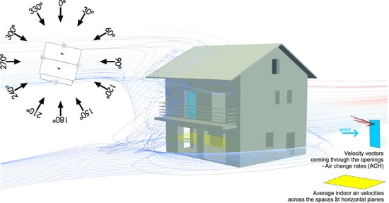
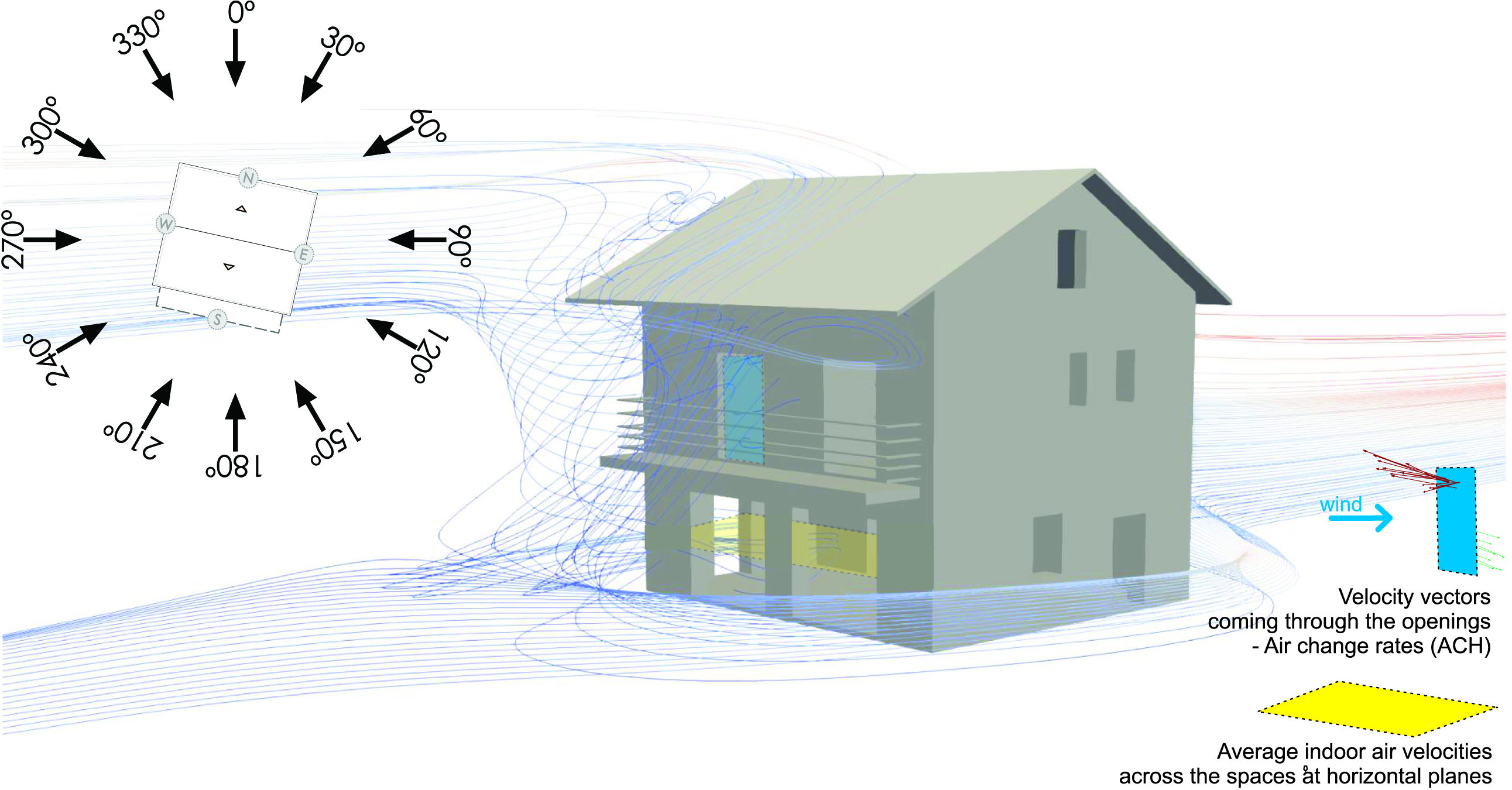
2.3. Wind Data Input for CFD Simulations

As wind direction fluctuates and significantly influences ventilation performance, experiments and simulations must consider its variation [79]. Thus, when defining the CFD boundary conditions for specific investigations/locations, it is essential to analyze the available wind data to outline the velocities and incident winds that are addressed at the numerical assessments. Considering this, the frequency distribution and wind speeds were initially extracted from the considered meteorological data. This analysis runs through the wind rose component from the parametric environmental plugin Ladybug [80], together with native Rhino/Grasshopper elements.

The component takes an EnergyPlus Weather file (.epw) as input, and how many cardinal points dividing the hourly average wind speed data must be defined. One needs at least four cardinal directions, and 36 angles (10° interval) would represent a high resolution. Data distribution between 30° to 40° is recommended in [81] to establish a direct relationship between the available wind angles and the best building orientation that could benefit from the winds. Thus, 12 cardinal directions were considered in this investigation. As output, the component gives a list containing the time-frequency that the wind is coming from for each direction and the average wind velocity. However, a logarithmic normal distribution is considered to better describe the probability distribution of the wind speed frequency curves [82,83]. Therefore, both normal and lognormal distributions were used (Figure 3) when analyzing the wind speed statistical distribution, and the best fit was selected. Each of these dominant incident wind directions corresponds to a building rotation angle that, together with its respective wind speed, configured a unique CFD model.

Besides the wind data from the experimental campaign (19-25.08.14), the investigations also considered the cooling season, identified from April to September [78], as a boundary condition. While the former compares simulated to measured data, the latter aims to take into account the period in which natural ventilation could be used as a cooling strategy, thus configuring a more representative analysis. In this sense, a statement condition function was applied to the Ladybug wind rose component for the cooling season, restricting the wind data assortment to the period when the dry-bulb temperature (DBT) was higher than 24 °C.

Figure 4 gathers the wind roses generated for both investigated scenarios, showing their respective wind speed and frequency values for each considered direction. Most of the wind speed distribution follows the logarithmic normal distribution, except for the southwest wind (θ = 240°) in the measurement week (Scenario 1) and θ = 60°, θ = 90°, and θ = 120° in the cooling season (Scenario 2). Figure 3b illustrates this exception, showing that the normal distribution best describes the east wind (θ = 90°) of the cooling season. In most cases, however, the lognormal distribution provides a better fit, as shown in Figure 3a, which illustrates the data of the south wind (θ = 180°) recorded in the measurement week.

As 12 directions are considered for each scenario, 24 CFD models are generated. Nevertheless, as this represents a high computational cost, the study was restricted to the most occurring wind directions. Therefore, the wind angles with frequencies less than 1.5% in the cooling period and 5% in the measurement week were not simulated, totaling 18 CFD models. The investigated angles (incident wind directions) in the study are highlighted in Figure 4.

3. CFD Model

3.1. Model Configuration

The CFD open-source code Field Operation and Manipulation OpenFOAM software [84], version 2006, was used to run a steady airflow through a three-dimensional model. As the study focused on wind-driven ventilation, the effects of thermal-driven ventilation (buoyancy) were not considered, meaning the simulations run under isothermal conditions. OpenFOAM has an extensive range of features to solve complex fluid flows and has been validated with both on-site measurements and wind-tunnel experimental data [85,86].

Conventionally, the simulation process takes place at the Grasshopper/Rhino interface, and the CFD engine runs in the background. This procedure, despite systematizing the calculation, has a downside: the program remains in processing until all simulation steps are finished. Therefore, considering the number of cases in this study, it was preferred to run them directly on the OpenFOAM terminal, using the Linux operating system. The use of Butterfly components was restricted to writing CFD model files, and instead of using command lines to execute the simulation steps, a script was developed to automatize the process.

3.1.1. Domain

Two geometries were developed for the study (Figure 5). One uses the window configurations from the experimental campaign to enable comparison between simulated and measured data (CFD 1—Figure 5b). As opposed to the cooling season model, all openings were left completely open, without frames (CFD 2—Figure 5c). This approach provides the maximum airflow rates in the spaces to assess if natural ventilation may be employed as a cooling strategy.

The model setup encompasses a coupled indoor–outdoor CFD simulation, where the same computational domain captures the dynamic interaction between external and internal environments around openings [61,87,88]. Based on the best practices guidelines [89], the computational domain size was determined: windward, height, and lateral sides = 5H, and leeward = 15 H to allow flow redevelopment; where H is the building height (8.5m). As a result, the computational domain (Figure 5a) had the following measurements: length × width × height, of 183 × 98 × 42 m³, resulting in a blockage ratio of 1.8%, which meets the recommended values by previous studies of less than 3%, to avoid the effect of compressed flow [89,90].

3.1.2. Solver Settings

We considered the flow as turbulent; therefore, a turbulence model, RANS equations [91], was employed for determining the wind pressure variations on the I-MA house, solved in combination with the standard k-ε turbulence model. Numerous studies investigated different CFD turbulence models to predict airflow in naturally ventilated buildings and revealed that the two-equation k-ε turbulence model is optimal from a performance/cost perspective compared to other models [52,92,93,94]. The k-ε turbulence model is one of the most commonly used two-equations turbulence model in CFD for natural ventilation problems, and it is described as stable, giving reasonably accurate results for most indoor airflows. However, it may have difficulties dealing with special room situations (e.g., high-buoyancy effect and large temperature gradient [51]), which is not the subject of this research.

For the velocity-pressure coupling, a steady-state solver for incompressible and turbulent flows was used—the semi-implicit method for pressure-linked equations (SIMPLE algorithm) [95]. The under-relaxation factors (α, 0 < α ≤ 1) were respectively set to 0.3 to pressure p, and 0.7 to velocity U, turbulent kinetic energy k, and dissipation rate ε. The under-relaxation technique is employed to improve computational stability, limiting the amount that the variable changes from one iteration to the next [96]. Second-order discretization schemes were used for both convection and diffusion terms of the mathematical governing equations. The selected numerical schemes set for these terms were correspondingly bounded Gauss linearUpwind [97] and the Gauss linear limited corrected, where the explicit non-orthogonal correction was set to Ψ = 0.333.

Both residuals values and monitoring results at specific locations (probes) were set as convergence criteria. For the latter, points located at the window surface area were selected, and the velocity and pressure outputs in those points were checked. The solutions converted approximately at the maximum residual level of 10⁻⁵ with solution imbalances of less than 0.5%. All CFD simulations were run using a desktop with 20 Cores and 288 GB of RAM memory. The computational time for each incident wind was approximately 7 min.

3.1.3. Mesh Processing and Boundary Conditions

The accuracy of the CFD results directly depends on the mesh quality, which was generated by the snappyHexMesh and the blockMesh utilities of OpenFOAM. First, blockMesh creates a background mesh that defines the domain extensions and a base level mesh. Afterward, snappyHexMesh constructs a three-dimensional polyhedral mesh around the investigated geometry described by a tri-surface mesh made of hexahedra cells. The computational grid was fully structured, being more refined near the area of interest, the immediate surroundings of the building model. Minimum and maximum layer thickness were 0.01 and 0.3, respectively, with an expansion ratio of 1.1, guaranteeing a smooth transition from fine mesh near the wall surfaces and avoiding significant aspect ratios that can compromise convergence. The resulting grid and mesh for both CFD models are shown in Figure 5b,c, which had four refinement levels and three cells between levels. Although the snappyHexMeshDict already contains numerous quality control settings, the mesh quality was also visually verified in ParaView [98] version 5.8.0, an open-source, multi-platform data analysis for visualization applications; and statistically assessed with the checkMesh utility of OpenFOAM. Other quality controls, such as maximum non-orthogonality and feature angles were also changed, set respectively to 50 and varying form 70–90, considering each of the incident wind direction simulated.

Moreover, grid sensitivity studies were conducted to ensure that the selected grid results did not vary considerably with finer grid resolutions. Therefore, coarse, medium, and fine meshes were created for CFD model 2 considering the north wind direction (θ = 0°) by changing the number of refinement levels. Consequently, the ratio between the smallest and largest mesh is beyond a conventional range, although the differences in results among them differ to the third decimal place.

Table 2. Grid sensitivity with CFD 2.

Mesh Type	Refine Levels	Cells Count	Mean Scalar Velocity (1st Floor)	Residuals
				Ux	Uy	Uz	p	Cumulative Continuity
1. Coarse	2,3	758,617	0.174975	4.1 × 10−5	2.5 × 10−7	4.1 × 10−5	3.3 × 10−3	1.068 × 10−8
2. Medium	3,4	1,225,845	0.1726165	3.6 × 10−5	3.0 × 10−7	2.9 × 10−5	3.8 × 10−3	1.061 × 10−8
3. Fine	4,5	3,880,640	0.171156	3.5 × 10−5	2.6 × 10−7	3.6 × 10−5	3.8 × 10−3	1.325 × 10−8

presents the total number of cells, model residuals, and the calculated mean scalar velocity values for the I-MA first floor. As the variance between the coarse and fine grid is close to 1.5% and between the medium and fine mesh is below 1%, all simulations utilized the medium mesh properties.

Regarding the boundary conditions, vertical profiles for the mean velocity U, turbulent kinetic energy k, and dissipation rate ε were assigned at the inlet through the atmospheric boundary layer (ABL) function [99]. As for the wind velocity, applied normal to the inlet, the values were set according to the wind data selection described previously in Section 2.3. With the ABL function, the roughness class and length (Z₀) of the area around the reference building is taken into account, where Z₀ = 0.25 corresponds to an area with scattered obstacles, e.g., low buildings [100], which is the case for the experimental building too.

Furthermore, standard wall functions were assigned for the ground and building surfaces, and the near-wall velocity profiles were modeled so that a transition between the fully turbulent area and the region near the wall is considered due to the turbulence models requiring complementary information in the near-wall region [101]. The non-dimensional parameter y+ that describes the treatment near the walls was measured in 58, which is within the best practice interval from 30 to 300 for k-ε turbulence model [102,103]. A zero-static pressure (fixedValue) was applied at the outlet plane, also assigned with a velocity inlet/outlet type. Zero normal velocities and zero-gradient pressures were set to the ground and building surfaces, while the top and lateral sides of the domain were set as slip, meaning the viscous effects at the wall are negligible on those regions.

3.2. Model Verification

To demonstrate the accuracy of the numerical simulations, velocity components predicted within the RANS model were compared against experimental results. The flow condition and building dimensions followed the wind tunnel experiment from Karava et al. [104], which used particle image velocimetry (PIV) to measure the velocity field inside a single zone. The full-scale model width, length, and height equal 20 × 20 × 16 m, respectively, with one opening (9.2 m × 3.6 m) at the center of the inlet and outlet facades (Configuration E1 [104]), modeled in 1:2 scale. All other settings of the CFD model were maintained as described in the previous sections. Figure 6 shows the simulation results and the experimental data of the normalized velocity U/U_ref distribution on a horizontal measurement line (L). The square symbols represent the PIV measurements of Karava et al. [104], and the x symbols are the simulation results of Ramponi and Blocken [87] with shear-stress transport (SST) k-ω model (their reference case). The mean absolute deviation between simulation and experimental data is 0.090 for the whole section but drops to 0.047 if restricted to the readings inside the investigated geometry. The comparison shows that Ux results agree with data from the reference study, and CFD can reproduce the velocity tendency.

4. Post-Processing

Natural ventilation is evaluated in three ways in this study: (i) average air velocities (m/s) in horizontal planes across the spaces; (ii) ACH, using either all velocity vectors that pass through the openings; or (iii) filtering recirculation of return air with the assistance of the parametric design platform, which also displays the velocity vectors.

4.1. Air Velocities

After the case has run and converged, OpenFOAM surface field value object functions are added to the system file, and the case runs once again so that average indoor air velocity (m/s) across all spaces are calculated at 1.2 m height horizontal plans (.stl files). These surfaces, shown in yellow in Figure 7a, are parametrically exported from the Rhino geometry file using Grasshopper plugins, which transformed the drawn plans into OpenFOAM object functions. The average wind speed calculated on each of the plans/rooms is saved as a sub-folder among the post-processing files. A MatLab script accesses these folders and collects the recorded results, grouping them according to their respective simulated incident wind direction.

4.2. ACH—Integration Method (All Velocity Vectors)

The multi-platform ParaView was used to fulfill two purposes: qualitative and quantitative analyses of results. While one allows a visual examination, observing airflows/velocity vectors, the other aims to calculate the ACH through the integration method. For this, the airflow rates (m³/s) are determined by applying the integrate variables filter in the vertical planes forming the openings crosssection of the investigated rooms within the three-dimensional CFD model. However, in ParaView, all vectors are computed, not just the positive ones, which can lead to calculation errors. Figure 7b shows these vertical planes (solid fill), and the red rectangle represents the slice plane that cuts one of the openings. The airflow is calculated in each of the room openings that, when added together, give the room ventilation rate (Equation (1)), converted to ACH using Equation (2).

4.3. ACH—Integration Method (Without Recirculation)

The primary goal was to visualize the velocity vectors coming through the openings, allowing for a comprehensive airflow assessment. For this, the following protocol was adopted: first, vector velocities (x, y, and z axes) that cross each point of the vertical openings section are exported as .csv files; second, a Grasshopper/Rhino definition imports both vectors and points, so one can visualize and analyze it. Grasshopper reads the ParaView .csv files and uses predefined geometry information in Rhino to plot the vector data in its respective vertical sections.

Additionally, the 3D parametric modeling tool allows filtering of the velocity vectors, accounting for just the positive velocities and so removing air recirculation. By using native Grasshopper components, the openings normal planes are identified, and only the velocity vectors entering the rooms are computed, discarding the recirculation flows, represented as red arrows in Figure 8.With this approach, the scalar velocity (m/s) in each opening area (m²) is estimated, determining volume flow (m³/s) and, consequently, the ACH in each of the investigated rooms. Recirculation flows are accounted as 0 m/s, and the total opening area is considered.

One limitation of this approach is that the surface opening must be completely free, which prevents the analysis of different window frames/configurations. Due to this limitation, the procedure was only applied to CFD 2 (cooling season scenario), where all openings were modeled without frames.

Moreover, both ParaView and Grasshopper working states allow for settings adjusted for one case to be replicated in others. Thus, only one post-processing definition was created to perform qualitative analyses in ParaView and import the .csv files in Grasshopper/Rhino. The most intensive task was generating the vector velocities (.csv files) for the ACH calculations, where the rotation angles needed to be updated for each of the different incident directions simulated at the CFD cases.

5. Results and Discussions

5.1. CFD 1—Measurement Week

Figure 9 illustrates the flow distribution for the most occurring wind direction (θ = 180°) at the I-MA house in a qualitative perspective, modeled after the window settings employed during measurements [78]. The dashed lines represent the measuring position over which the predicted indoor air velocities for each of the investigated wind directions were plotted (Figure 10 and Figure 11), and the rectangle defines the region covered by the anemometer.

First, the indoor air velocities (m/s) recorded in the living room were screened so that the experimental campaign measurements could be related to the CFD 1 outputs. In this sense, data recorded with closed windows (7:00 a.m.–8:59 p.m.) were excluded, and the remaining readings were grouped and averaged given the same angle range used in CFD simulations, resulting in a single measured value for each wind direction. Therefore, the values predicted by the CFD simulations along the line (several points) are compared to a resultant unique reading measured with the anemometer during the experiment.

The way the windows were left open (in a tilted position) during the measurements provided a greater airflow near the walls with lower speeds in the center of the rooms where the sensor was placed. Moreover, since most windows were closed during the experiment, slow velocities can be observed, with a maximum recorded value of 0.076 m/s, at the incident wind direction θ = 90° and a minimum of 0.062 m/s at θ = 30° and θ = 240°.

Figure 12 summarizes the resulting single air velocities measured with the anemometer and the averaged air velocities calculated by the CFD models in the horizontal plane (1.2 m above the floor) for the living room as solid and pattern bars, respectively, for four wind directions.

As the building ventilation system (no-load supply) was in operation throughout the experiment, even in the occurrence of external calm winds, air velocity measurements remained around 0.065 m/s, which does not necessarily indicate natural ventilation but rather an effect of the mechanized system. This is the case of incident winds at θ = 150°, θ = 180°, θ = 210°, and θ = 240° that have wind speed boundary condition assigned as less than 1.5 m, and the mechanized ventilation prevails over natural. As the artificial flow was not modeled, CFD simulations output indoor air velocities much slower than those measured, differing by about 30%. Therefore, these wind directions are not used as a reference comparison to the numerical model results and are not presented in Figure 12.

Nevertheless, while the air velocities across the spaces were non-uniform, varying significantly along the longitudinal axis, the average values calculated in the horizontal planes are a reasonable representation of indoor airflows. The representation efficiently captures the room ventilation performance, providing a more comprehensive analysis than that coming from a single sensor, restricted to a small accuracy. Hence, calculation planes configure a convenient and reliable method when assessing natural ventilation performance, in both building assessment or even in the project development phase.

5.2. CFD 2—Cooling Season

• Air velocities

In Figure 13, the air velocities calculated in the horizontal planes (1.2 m above the floor) for the cellar (C), living room (LV), and the three bedrooms (BR 1-3) are shown as bars for all ten incident wind directions investigated, and the inlet wind speed used in each angle is presented as a dotted line. The internal airflow varies significantly due to wind direction fluctuations being more sensitive to the direction than the outdoor wind speed, as demonstrated in [62]. For example, the cellar presents both the highest and lowest predicted indoor air velocities, 0.88 m/s and 0.08 m/s for incident wind directions θ = 0° and θ = 270°, respectively.

Considering all the investigated rooms, air velocities vary from 0.1 to 0.4 m/s, with an average value around 0.34 m/s on the ground floor (cellar (C) and living room (LR)) and 0.23 m/s on the first floor (bedroom 1–3 (BR1–BR3)), which, besides smaller openings, also has a balcony. Within this air velocity range, internal operative temperatures up to 28 °C would be acceptable according to comfort standards. However, other passive or active strategies must be utilized in higher temperatures, such as buoyancy-driven airflows or fans.

The wind direction’s influence on the air flows and the predicted air velocities can be observed in Figure 14. The image combines the distribution of normalized mean wind speed U_norm (the mean wind speed values were rescaled to have mean = 0 and standard deviation = 1) and streamlines patterns around the ground and first floor. For the sake of space, only the three most frequent incident wind directions (θ = 150°, 180°, 210°) and the highest speed (θ = 0°) are portrayed. Both predicted U_norm and streamlines vary significantly with incident wind directions in terms of eddies’ existence, size, and position in the rooms. Depending on the incident wind angle, the flows in space may present either a pattern from a cross-ventilated room, with a more uniform distribution (Figure 14c,e, or of a single-sided one, showing eddy formations in the room corners (Figure 14a,g).

Moreover, higher indoor air velocities are observed when the building orientation is oblique to an incident wind angle. The case with the south wind (θ = 180°), for example, perpendicular to the building’s openings (Figure 14e,f)), presents lower air velocity values than the oblique one, with the south-southwest direction (θ = 210°) (Figure 14g,h), although both have the same inlet wind speed of 1.55 m/s. While the bedrooms 1 and 2 show air velocities of 0.11 and 0.25 m/s for θ = 180°, when θ = 210°, the values are 0.26 and 0.34 m/s, respectively. This influence of the building orientation concerning the wind incident angle is also observed in [18].

• ACH—Integration Method

A comparison between the ACH calculated with the two integration methods described in Section 4.2 and Section 4.3 is presented in Figure 15. for the living room, cellar, and bedrooms 1 and 2. Bedroom 3 is omitted for brevity and because it shows a similar airflow behavior as bedroom 2.

A direct relationship can be observed between the predicted velocities calculated in the horizontal plane (Figure 14) and the ACH estimated with the integration method. At the same time, the ventilation rates restricted to the velocity vectors entering the room (dotted line with square markers) are in general lower in the ground floor and bigger in the first floor than those using all velocities that pass through the openings (continuous lines with cross-markers). As the ACH values depend on the room volume, the living room (65.7 m³) presents the lowest air rates, varying from 1.66 to 2.8 (ACH⁻¹), using the method described in the Section 4.2, against 1.6 to 3.3 (ACH⁻¹) when disregarding recirculation flows (Section 4.3). Despite the different ventilation rates found in each incident wind direction, filtered ACH values calculated by combining CFD results to Grasshopper components vary, on average, between −11% to +6%, which can impact performance assessments. In Appendix A, Figure A1 shows the visualization in Rhino of the average normal velocities coming through the openings for the south wind direction (θ = 180°).

6. Research Constraints and Remarks

This study employs CFD to explore wind-driven natural ventilation through 3D parametric modeling platforms. Accuracy of the assessment process is ensured by carefully defining the boundary conditions and numerical settings, besides comparing CFD results (velocity components and indoor air velocities) with data from a wind tunnel experiment and a large-scale measurement campaign. Nevertheless, future studies and design applications must consider some limitations regarding this investigation, including:

• Assessment of natural ventilation occurred in wind-driven conditions. Different solver settings and boundary conditions are required to investigate buoyancy-driven ventilation.
• The CFD domain did not include immediate surroundings. For analyses in an urban context, modeling the neighborhood should be considered.
• The influence of window opening degree was not investigated, since all openings were modeled without frames opened. This approach delivers the maximum ventilation potential of the building. However, as window operation influences natural ventilation performance [105], window opening schedules could be modeled for a more precise assessment, when known.
• The current study measured air velocity (m/s) and used RANS and k-ε turbulence models in the investigations. Despite its effectiveness, a different approach would be required to properly verify the ACH calculated by the adapted integration method described in Section 4.3. Some alternatives include using LES or other turbulence models such as shear-stress transport (SST) k-ω associated with physical experimentation involving airflow prediction through the tracer-gas decay method. Testing different turbulence models comprise the scope of future work.
• Displaying velocity vectors within the 3D parametric design software is an alternative in light of qualitative airflow evaluations. However, further experimental campaigns should be programmed for tracer-gas measurements besides deeper investigations to allow for checking the accuracy of the approach when employed to solve the integration method excluding recirculation flows.

Finally, some advantages and disadvantages of integrating parametric 3D modeling with CFD are highlighted, compared to conventional CFD models:

Pros:

• The CFD workflow and tasks are organized with visual programming resources rather than code lines, allowing a better understanding of their steps, especially for users unfamiliar with conventional programming languages.
• The integration between the project’s geometry and the CFD model’s automatic generation facilitates performing CFD simulations during either project development or building performance assessment. As the tools are embedded in a single platform, parameterized geometric configurations can be easily changed and tested.
• Several configurations are pre-established within the CFD plugin in the 3D software and have default values based on natural ventilation studies’ best practices. Therefore, designers can perform CFD simulations with more reliability. Nonetheless, it is possible to change or add new functions using all OpenFOAM capabilities. As a result, advanced users can adapt their models as desired and profit from the 3D parametric resources.

Cons:

• Although OpenFOAM is a free, open-source platform, the proposed CFD workflow needs a commercial 3D modeling software.
• Compared to other commercial CFD programs, such as Ansys-Fluent and CFX, the number of predetermined features to set up a model with the 3D modeling platform’s CFD plugin is smaller. Hence, the user might have to make a more significant effort when trying to model a problem outside the available files and settings.

7. Conclusions

This paper presented a framework to systematize the analyses of a building’s wind-driven natural ventilation potential through CFD simulation. Combining available programs and developing customized functions, the study provided a pragmatic use of CFD for either building design or assessment. A full-scale test house was used as a base case, its geometry and the climatic characteristics of its site were settled as a reference, and air velocity measurements performed within the experimental house served as validation data. Insights regarding the procedure that covers from pre- to post-processing steps include:

• The proposed workflow assists practical use of CFD, combining more accessible wind-driven airflow simulation resources and an oriented method, which can promote CFD applications at the design phase and encourage comprehensive building evaluations.
• The detailed information regarding wind data definition and numerical model settings can help future studies and applications willing to use CFD in natural ventilation assessments.
• Combining 3D modeling platform utilities with CFD objective functions to generate parameterized calculation surfaces automates post-processing and accelerates the analysis. It provides an effective quantitative way to investigate naturally ventilated buildings with CFD.

Lastly, the CFD simulations provided information on the ventilative effectiveness of the test house, used as a reference building in this study. The results lead to the following conclusions:

• Since air velocities across the room are non-uniform, the horizontal calculation plans provide a quick but rather general space reference value. For a more detailed analysis, one must check velocity contours and streamlines.
• For the cooling season, 10 of the 12 wind directions considered at the climactic analysis were simulated, preferring those most frequent. Although the number of wind directions to be considered is adjustable, it is noted that wind direction fluctuations considerably influence the internal airflow. Therefore, the greater the number of incident wind directions, the better the building characterization. However, if one must limit cases, prioritizing the oblique winds based on occurrence would be recommended as they are more effective for open windows.

References

1. Zhu, Y.; Luo, M.; Ouyang, Q.; Huang, L.; Cao, B. Dynamic characteristics and comfort assessment of airflows in indoor environments: A review. Build. Environ. 2015, 91, 5–14. [Google Scholar] [CrossRef]
2. Sundell, J.; Levin, H.; Nazaroff, W.W.; Cain, W.S.; Fisk, W.J.; Grimsrund, D.T.; Gyntelberg, F.; Li, Y.; Persily, A.K.; Pickering, A.C. Ventilation rates and health: Multidisciplinary review of the scientific literature. Indoor Air 2011, 21, 191–204. [Google Scholar] [CrossRef] [PubMed]
3. Chenari, B.; Dias Carrilho, J.; Gameiro da Silva, M. Towards sustainable, energy-efficient and healthy ventilation strategies in buildings: A review. Renew. Sustain. Energy Rev. 2016, 59, 1426–1447. [Google Scholar]
4. European Commission. Ventilation, Good Indoor Air Quality and Rational Use of Energy, Report No 23; European Commission: Brussels, Belgium, 2003. [Google Scholar]
5. DIN EN 16798-7. Energy Performance of Buildings-Ventilation For Buildings-Part 7: Calculation Methods For the Determination of Air Flow Rates in Buildings Including Infiltration; DIN EN: Berlin, Germany, 2017. [Google Scholar]
6. ASHRAE. Standard 62.1-2016: Ventilation for Acceptable Indoor Air Quality; American Society of Heating, Refrigerating and Air-Conditioning Engineers: Atlanta, GA, USA, 2016. [Google Scholar]
7. CIBSE. Applications Manual AM 10. Natural Ventilation in Non-Domestic Buildings; Chartered Institution of Building Services Engineers: London, UK, 2010. [Google Scholar]
8. CIBSE. Guide A. Environmental Design; Chartered Institution of Building Services Engineers: London, UK, 2007. [Google Scholar]
9. de Faria, L.C.; Cook, M.J.; Loveday, D.; Angelopoulos, C.; Shukla, Y.; Rawal, R.; Manu, S.; Mishra, D.; Patel, J.; Anbarasu, S. Design Charts to Assist on the Sizing of Natural Ventilation for Cooling Residential Apartments in India. In Proceedings of the 16th International Building Simulation Conference, Rome, Italy, 2–4 September 2019; pp. 696–703. [Google Scholar]
10. Faggianelli, G.A.; Brun, A.; Wurtz, E.; Muselli, M. Natural cross ventilation in buildings on Mediterranean coastal zones. Energy Build 2014, 77, 206–218. [Google Scholar] [CrossRef]
11. Kiwan, A.; Berg, W.; Brunsch, R.; Özcan, S.; Müller, H.-J.; Gläser, M.; Fiedler, M.; Ammon, C.; Berckmans, D. Tracer gas technique, air velocity measurement and natural ventilation method for estimating ventilation rates through naturally ventilated barns. Agric. Eng. Int. 2012, 14, 22–36. [Google Scholar]
12. Brambilla, A.; Bonvin, J.; Flourentzou, F.; Jusselme, T. On the Influence of Thermal Mass and Natural Ventilation on Overheating Risk in Offices. Build. 2018, 8, 47. [Google Scholar] [CrossRef] [Green Version]
13. Mateus, N.M.; Simões, G.N.; Lúcio, C.; da Graça, G.C. Comparison of measured and simulated performance of natural displacement ventilation systems for classrooms. Energy Build. 2016, 133, 185–196. [Google Scholar] [CrossRef]
14. Weerasuriya, A.U.; Zhang, X.; Gan, V.J.L.; Tan, Y. A holistic framework to utilize natural ventilation to optimize energy performance of residential high-rise buildings. Build. Environ. 2019, 153, 218–232. [Google Scholar] [CrossRef]
15. Johnson, M.-H.; Zhai, Z.; Krarti, M. Performance evaluation of network airflow models for natural ventilation. HVAC&R Res. 2012, 18, 349–365. [Google Scholar]
16. Sakiyama, N.R.M.; Carlo, J.C.; Frick, J.; Garrecht, H. Perspectives of naturally ventilated buildings: A review. Renew. Sustain. Energy Rev. 2020, 130, 109933. [Google Scholar] [CrossRef]
17. Chen, Q. Ventilation performance prediction for buildings: A method overview and recent applications. Build. Environ. 2009, 44, 848–858. [Google Scholar] [CrossRef]
18. Porras-Amores, C.; Mazarrón, F.R.; Cañas, I.; Villoría Sáez, P. Natural ventilation analysis in an underground construction: CFD simulation and experimental validation. Tunn. Undergr. Space Technol. 2019, 90, 162–173. [Google Scholar] [CrossRef]
19. Albuquerque, D.P.; Mateus, N.; Avantaggiato, M.; Carrilho da Graça, G. Full-scale measurement and validated simulation of cooling load reduction due to nighttime natural ventilation of a large atrium. Energy Build. 2020, 224, 110233. [Google Scholar] [CrossRef]
20. You, W.; Qin, M.; Ding, W. Improving building facade design using integrated simulation of daylighting, thermal performance and natural ventilation. Build. Simul. 2013, 6, 269–282. [Google Scholar] [CrossRef]
21. Hong, T.; Lee, M.; Kim, J. Analysis of Energy Consumption and Indoor Temperature Distributions in Educational Facility Based on CFD-BES Model. Energy Procedia 2017, 105, 3705–3710. [Google Scholar] [CrossRef]
22. Elshafei, G.; Negm, A.; Bady, M.; Suzuki, M.; Ibrahim, M.G. Numerical and experimental investigations of the impacts of window parameters on indoor natural ventilation in a residential building. Energy Build. 2017, 141, 321–332. [Google Scholar] [CrossRef]
23. Raji, B.; Tenpierik, M.J.; Bokel, R.; van den Dobbelsteen, A. Natural summer ventilation strategies for energy-saving in high-rise buildings: A case study in the Netherlands. Int. J. Vent. 2020, 19, 25–48. [Google Scholar] [CrossRef] [Green Version]
24. Blocken, B. Computational Fluid Dynamics for urban physics: Importance, scales, possibilities, limitations and ten tips and tricks towards accurate and reliable simulations. Build. Environ. 2015, 91, 219–245. [Google Scholar] [CrossRef] [Green Version]
25. de Faria, L.C.; Cook, M.J.; Loveday, D.; Angelopoulos, C.; Manu, S.; Shukla, Y. Sizing natural ventilation systems for cooling: The potential of NV systems to deliver thermal comfort while reducing energy demands of multi-storey residental buildings in india. In Proceedings of the 34th Passive and Low Energy Architecture Conference, HongKong, China, 10–12 December 2018; pp. 218–224. [Google Scholar]
26. Hawendi, S.; Gao, S. Impact of an external boundary wall on indoor flow field and natural cross-ventilation in an isolated family house using numerical simulations. J. Build. Eng. 2017, 10, 109–123. [Google Scholar] [CrossRef] [Green Version]
27. Ferrucci, M.; Brocato, M. Parametric analysis of the wind-driven ventilation potential of buildings with rectangular layout. Build. Serv. Eng. Res. Technol. 2019, 40, 109–128. [Google Scholar] [CrossRef]
28. Yang, T.; Wright, N.G.; Etheridge, D.W.; Quinn, A.D. A Comparison of CFD and Full-scale Measurements for Analysis of Natural Ventilation. Int. J. Vent. 2006, 4, 337–348. [Google Scholar] [CrossRef]
29. El Ahmar, S.; Battista, F.; Fioravanti, A. Simulation of the thermal performance of a geometrically complex Double-Skin Facade for hot climates: EnergyPlus vs. OpenFOAM. Build. Simul. 2019, 2, 781–795. [Google Scholar] [CrossRef]
30. Ferrucci, M.; Brocato, M.; Peron, F. Digital Tools for the Morphological Design of the Naturally Ventilated Buildings. Future Cities Environ. 2018, 4, 478. [Google Scholar] [CrossRef] [Green Version]
31. Kim R-w Hong S-w Norton, T.; Amon, T.; Youssef, A.; Berckmans, D.; Lee, I. Computational fluid dynamics for non-experts: Development of a user-friendly CFD simulator (HNVR-SYS) for natural ventilation design applications. Biosyst. Eng. 2020, 193, 232–246. [Google Scholar] [CrossRef]
32. Ramponi, R.; Angelotti, A.; Blocken, B. Energy saving potential of night ventilation: Sensitivity to pressure coefficients for different European climates. Appl. Energy 2014, 123, 185–195. [Google Scholar] [CrossRef]
33. Chu, C.-R.; Chiang, B.-F. Wind-driven cross ventilation in long buildings. Build. Environ. 2014, 80, 150–158. [Google Scholar] [CrossRef]
34. Chu, C.-R.; Chiang, B.-F. Wind-driven cross ventilation with internal obstacles. Energy Build. 2013, 67, 201–209. [Google Scholar] [CrossRef]
35. Bangalee, M.Z.I.; Lin, S.Y.; Miau, J.J. Wind driven natural ventilation through multiple windows of a building: A computational approach. Energy Build. 2012, 45, 317–325. [Google Scholar] [CrossRef]
36. Shirzadi, M.; Mirzaei, P.A.; Naghashzadegan, M.; Tominaga, Y. Modelling enhancement of cross-ventilation in sheltered buildings using stochastic optimization. Int. J. Heat Mass Transf. 2018, 118, 758–772. [Google Scholar] [CrossRef]
37. Zhong, H.-Y.; Jing, Y.; Sun, Y.; Kikumoto, H.; Zhao, F.-Y.; Li, Y. Wind-driven pumping flow ventilation of highrise buildings: Effects of upstream building arrangements and opening area ratios. Sci. Total. Environ. 2020, 722, 137924. [Google Scholar] [CrossRef] [PubMed]
38. Arinami, Y.; Akabayashi, S.-i.; Tominaga, Y.; Sakaguchi, J. Performance evaluation of single-sided natural ventilation for generic building using large-eddy simulations: Effect of guide vanes and adjacent obstacles. Build. Environ. 2019, 154, 68–80. [Google Scholar] [CrossRef]
39. Zheng, J.; Tao, Q.; Li, L. Numerical study of wind environment of a low-rise building with shading louvers: Sensitive analysis and evaluation of cross ventilation. J. Asian Archit. Build. Eng. 2020, 19, 541–558. [Google Scholar] [CrossRef]
40. Castillo, J.A.; Huelsz, G.; van Hooff, T.; Blocken, B. Natural ventilation of an isolated generic building with a windward window and different windexchangers: CFD validation, sensitivity study and performance analysis. Build. Simul. 2019, 12, 475–488. [Google Scholar] [CrossRef]
41. Gautam, K.R.; Rong, L.; Zhang, G.; Abkar, M. Comparison of analysis methods for wind-driven cross ventilation through large openings. Build. Environ. 2019, 154, 375–388. [Google Scholar] [CrossRef]
42. Pakari, A.; Ghani, S. Airflow assessment in a naturally ventilated greenhouse equipped with wind towers: Numerical simulation and wind tunnel experiments. Energy Build. 2019, 199, 1–11. [Google Scholar] [CrossRef]
43. Dai, Y.W.; Mak, C.M.; Ai, Z.T. Computational fluid dynamics simulation of wind-driven inter-unit dispersion around multi-storey buildings: Upstream building effect. Indoor Built Environ. 2019, 28, 217–234. [Google Scholar] [CrossRef] [Green Version]
44. Gough, H.; King, M.-F.; Nathan, P.; Grimmond, C.S.B.; Robins, A.; Noakes, C.J.; Luo, C.; Barlow, J.F. Influence of neighbouring structures on building façade pressures: Comparison between full-scale, wind-tunnel, CFD and practitioner guidelines. J. Wind Eng. Ind. Aerodyn. 2019, 189, 22–33. [Google Scholar] [CrossRef] [Green Version]
45. Hirose, C.; Ikegaya, N.; Hagishima, A.; Tanimoto, J. Outdoor measurement of wall pressure on cubical scale model affected by atmospheric turbulent flow. Build. Environ. 2019, 160, 106170. [Google Scholar] [CrossRef]
46. Lo, L.J.; Novoselac, A. Cross ventilation with small openings: Measurements in a multi-zone test building. Build. Environ. 2012, 57, 377–386. [Google Scholar] [CrossRef]
47. Hayati, A.; Mattsson, M.; Sandberg, M. A wind tunnel study of wind-driven airing through open doors. Int. J. Vent. 2019, 18, 113–135. [Google Scholar] [CrossRef] [Green Version]
48. Tecle, A.; Bitsuamlak, G.T.; Jiru, T.E. Wind-driven natural ventilation in a low-rise building: A Boundary Layer Wind Tunnel study. Build. Environ. 2013, 59, 275–289. [Google Scholar] [CrossRef]
49. Shirzadi, M.; Tominaga, Y.; Mirzaei, P.A. Wind tunnel experiments on cross-ventilation flow of a generic sheltered building in urban areas. Build. Environ. 2019, 158, 60–72. [Google Scholar] [CrossRef]
50. Hensen, J.; Lamberts, R. Building Performance Simulation for Design and Operation; Spon Press: London, UK; New York, NY, USA, 2011. [Google Scholar]
51. Zhai, Z.J.; Zhang, Z.; Zhang, W.; Chen, Q.Y. Evaluation of Various Turbulence Models in Predicting Airflow and Turbulence in Enclosed Environments by CFD: Part 1—Summary of Prevalent Turbulence Models. HVAC&R Res. 2007, 13, 853–870. [Google Scholar] [CrossRef]
52. Zhang, Z.; Zhang, W.; Zhai, Z.J.; Chen, Q.Y. Evaluation of Various Turbulence Models in Predicting Airflow and Turbulence in Enclosed Environments by CFD: Part 2—Comparison with Experimental Data from Literature. HVAC&R Res. 2007, 13, 871–886. [Google Scholar] [CrossRef]
53. Jiang y Alexander, D.; Jenkins, H.; Arthur, R.; Chen, Q. Natural ventilation in buildings: Measurement ina wind tunnel and numerical simulation with large-eddy simulation. J. Wind. Eng. Ind. Aerodyn. 2003, 91, 331–353. [Google Scholar] [CrossRef]
54. Jiang y Chen, Q. Study of natural ventilation in buildings by large eddy simulation. J. Wind Eng. Ind. Aerodyn. 2001, 89, 1155–1178. [Google Scholar] [CrossRef] [Green Version]
55. Wright, N.G.; Hargreaves, D.M. Unsteady CFD Simulations for Natural Ventilation. Int. J. Vent. 2006, 5, 13–20. [Google Scholar] [CrossRef]
56. Bu, Z.; Kato, S. Wind-induced ventilation performances and airflow characteristics in an areaway-attached basement with a single-sided opening. Build. Environ. 2011, 46, 911–921. [Google Scholar] [CrossRef]
57. Sherman, M.H. Tracer-gas techniques for measuring ventilation in a single zone. Build. Environ. 1990, 25, 365–374. [Google Scholar] [CrossRef]
58. Laußmann, D.; Helm, D. Air Change Measurements Using Tracer Gases: Methods and Results. Significance of Air Change for Indoor Air Quality; Epidemiologie und Gesundheitsberichterstattung, Robert Koch-Institut: Berlin, Germany, 2011. [Google Scholar]
59. Caciolo, M.; Stabat, P.; Marchio, D. Numerical simulation of single-sided ventilation using RANS and LES and comparison with full-scale experiments. Build. Environ. 2012, 50, 202–213. [Google Scholar] [CrossRef]
60. Zhang, X.; Weerasuriya, A.U.; Tse, K.T. CFD simulation of natural ventilation of a generic building in various incident wind directions: Comparison of turbulence modelling, evaluation methods, and ventilation mechanisms. Energy Build. 2020, 229, 110516. [Google Scholar] [CrossRef]
61. Tong, Z.; Chen, Y.; Malkawi, A. Defining the Influence Region in neighborhood-scale CFD simulations for natural ventilation design. Appl. Energy 2016, 182, 625–633. [Google Scholar] [CrossRef]
62. Deng, X.; Tan, Z. Numerical analysis of local thermal comfort in a plan office under natural ventilation. Indoor Built Environ. 2020, 29, 972–986. [Google Scholar] [CrossRef]
63. Subhashini, S.; Thirumaran, K. CFD simulations for examining natural ventilation in the learning spaces of an educational building with courtyards in Madurai. Build. Serv. Eng. Res. Technol. 2020, 41, 466–479. [Google Scholar] [CrossRef]
64. Saadatjoo, P.; Mahdavinejad, M.; Zhang, G. A study on terraced apartments and their natural ventilation performance in hot and humid regions. Build. Simul. 2018, 11, 359–372. [Google Scholar] [CrossRef]
65. Cândido, C.; de Dear, R.; Lamberts, R. Combined thermal acceptability and air movement assessments in a hot humid climate. Build. Environ. 2011, 46, 379–385. [Google Scholar] [CrossRef]
66. Huang, L.; Ouyang, Q.; Zhu, Y.; Jiang, L. A study about the demand for air movement in warm environment. Build. Environ. 2013, 61, 27–33. [Google Scholar] [CrossRef]
67. Bayoumi, M. Improving Natural Ventilation Conditions on Semi-Outdoor and Indoor Levels in Warm–Humid Climates. Buildings 2018, 8, 75. [Google Scholar] [CrossRef] [Green Version]
68. ASHRAE. Standard 55: Thermal Environmental Conditions for Human Occupancy; ASHRAE: New York, NY, USA, 2013. [Google Scholar]
69. DIN EN 16798-1. Energy Performance of Buildings-Ventilation for Buildings-Part 1: Indoor Environmental Input Parameters for Design and Assessment of Energy Performance of Buildings Addressing Indoor Air Quality, Thermal Environment, Lighting and Acoustics-Module M1-6.(16798-1); DIN EN: Berlin, Germany, 2019. [Google Scholar]
70. Spentzou, E.; Cook, M.J.; Emmitt, S. Modelling natural ventilation for summer thermal comfort in Mediterranean dwellings. Int. J.Vent. 2019, 18, 28–45. [Google Scholar] [CrossRef] [Green Version]
71. Robert McNeel & Associates Rhinoceros 3D 5 for Windows and Mac, Seattle, WA, USA. Available online: https://www.rhino3d.com/ (accessed on 23 November 2020).
72. Davidson, S. Grasshopper. Available online: https://www.grasshopper3d.com/ (accessed on 23 November 2020).
73. Wang, B.; Malkawi, A. Genetic Algorithm Based Building Form Optimization Study for Natural Ventilation Potential. In Proceedings of the 14th International Building Simulation Conference, Hyderabad, India, 7–9 December 2015; pp. 640–647. [Google Scholar]
74. Yoon, N.; Piette, M.A.; Han, J.M.; Wu, W.; Malkawi, A. Optimization of Window Positions for Wind-Driven Natural Ventilation Performance. Energies 2020, 13, 2464. [Google Scholar] [CrossRef]
75. Mackey, C.; Galanos, T.; Norford, L.; Roudsari, M.S. Wind, Sun, Surface Temperature, and Heat Island: Critical Variables for High-resolution Outdoor Thermal Comfort. In Proceedings of the 15th International Building Simulation Conference, San Francisco, CA, USA, 7–9 August 2017; pp. 985–993. [Google Scholar]
76. Ganji, H.B.; Utzinger, D.M.; Bradley, D.E. Create and Validate Hybrid Ventilation Components in Simulation using Grasshopper and Python in Rhinoceros. In Proceedings of the 16th International Building Simulation Conference, Rome, Italy, 2–4 September 2019; pp. 4345–4352. [Google Scholar]
77. Roudsari, M.S.; Mackey, C. Butterfly. Ladybug Tools Butterfly. Available online: https://www.ladybug.tools/butterfly.html (accessed on 23 November 2020).
78. Sakiyama, N.R.M.; Mazzaferro, L.; Carlo, J.C.; Bejat, T.; Garrecht, H. Natural ventilation potential from weather analyses and building simulation. Energy Build. 2020, 231, 110596. [Google Scholar] [CrossRef]
79. Ji, L.; Tan, H.; Kato, S.; Bu, Z.; Takahashi, T. Wind tunnel investigation on influence of fluctuating wind direction on cross natural ventilation. Build. Environ. 2011, 46, 2490–2499. [Google Scholar] [CrossRef]
80. Roudsari, M.S.; Pak, M.; Smith, A. Ladybug: A parametric environmental plugin for grasshopper to help designers create an environmentally-conscious design. In Proceedings of the 13th International Building Simulation Conference, Chambéry, France, 26–28 August 2013; pp. 3128–3135. [Google Scholar]
81. Gandemer, J.; Barnaud, G. Guide Sur La Climatisation Naturelle De l’habitat En Climat Tropical Humide; Centre Scientifique Et Technique Du Bâtiment: Marne LaVale, France, 1997. [Google Scholar]
82. Calif, R.; Schmitt, F.G. Modeling of atmospheric wind speed sequence using a lognormal continuous stochastic equation. J. Wind Eng. Ind. Aerodyn. 2012, 109, 1–8. [Google Scholar] [CrossRef]
83. Garcia, A.; Torres, J.L.; Prieto, E.; Francisco, A.D.E. Fitting wind speed distributions: A case study. Sol. Energy 1998, 62, 139–144. [Google Scholar] [CrossRef]
84. OpenCFD Ltd. OpenFOAM: v1219 User Guide Openfoam. Available online: https://www.openfoam.com/documentation/user-guide/ (accessed on 23 November 2020).
85. Gartmann, A.; Fister, W.; Schwanghart, W.; Müller, M.D. CFD modelling and validation of measured wind field data in a portable wind tunnel. Aeolian Res. 2011, 3, 315–325. [Google Scholar] [CrossRef]
86. Kubilay, A.; Derome, D.; Blocken, B.; Carmeliet, J. Numerical simulations of wind-driven rain on an array of low-rise cubic buildings and validation by field measurements. Build. Environ. 2014, 81, 283–295. [Google Scholar] [CrossRef] [Green Version]
87. Ramponi, R.; Blocken, B. CFD simulation of cross-ventilation for a generic isolated building: Impact of computational parameters. Build. Environ. 2012, 53, 34–48. [Google Scholar] [CrossRef]
88. Tan, G.; Glicksman, L.R. Application of integrating multi-zone model with CFD simulation to natural ventilation prediction. Energy Build. 2005, 37, 1049–1057. [Google Scholar] [CrossRef]
89. Tominaga, Y.; Mochida, A.; Yoshie, R.; Kataoka, H.; Nozu, T.; Yoshikawa, M.; Shirasawa, T. AIJ guidelines for practical applications of CFD to pedestrian wind environment around buildings. J. Wind Eng. Ind. Aerodyn. 2008, 96, 1749–1761. [Google Scholar] [CrossRef]
90. Muhsin, F.; Yusoff, W.F.M.; Mohamed, M.F.; Sapian, A.R. CFD modeling of natural ventilation in a void connected to the living units of a multi-storey housing for thermal comfort. Energy Build. 2017, 144, 1–16. [Google Scholar] [CrossRef]
91. Cebeci, T.; Shao, J.P.; Kafyeke, F.; Laurendeau, E. Computational Fluid Dynamics for Engineers: From Panel to navier-Stokes Methods with Computer Programs; Springer Berlin Heidelberg: Heidelberg, Germany, 2005. [Google Scholar]
92. Chen, Q.; Lee, K.; Mazumdar, S.; Poussou, S.; Wang, L.; Wang, M.; Zhang, Z. Ventilation performance prediction for buildings: Model assessment. Build. Environ. 2010, 45, 295–303. [Google Scholar] [CrossRef] [Green Version]
93. Cheung, J.O.P.; Liu, C.-H. CFD simulations of natural ventilation behaviour in high-rise buildings in regular and staggered arrangements at various spacings. Energy Build. 2011, 43, 1149–1158. [Google Scholar] [CrossRef]
94. Farea, T.G.; Ossen, D.R.; Alkaff, S.; Kotani, H. CFD modeling for natural ventilation in a lightwell connected to outdoor through horizontal voids. Energy Build. 2015, 86, 502–513. [Google Scholar] [CrossRef]
95. Patankar, S.V.; Spalding, D.B. A calculation procedure for heat, mass and momentum transfer in three-dimensional parabolic flows. Int. J. Heat Mass Transf. 1972, 15, 1787–1806. [Google Scholar] [CrossRef]
96. Versteeg, H.K.; Malalasekera, W. An Introduction to Computational Fluid Dynamics: The Finite Volume Method, 2nd ed.; Pearson Education Ltd.: Harlow, UK; New York, NY, USA, 2007. [Google Scholar]
97. Warming, R.F.; Beam, R.M. Upwind Second-Order Difference Schemes and Applications in Aerodynamic Flows. AIAA J. 1976, 14, 1241–1249. [Google Scholar] [CrossRef]
98. Kitware Inc. ParaView. Available online: https://www.paraview.org/ (accessed on 23 November 2020).
99. Hargreaves, D.M.; Wright, N.G. On the use of the k– model in commercial CFD software to model the neutral atmospheric boundary layer. J. Wind Eng. Industrial Aerodyn. 2007, 95, 355–369. [Google Scholar] [CrossRef]
100. Hammond, D.S.; Chapman, L.; Thornes, J.E. Roughness length estimation along road transects using airborne LIDAR data. Meteorol. Appl. 2012, 19, 420–426. [Google Scholar] [CrossRef]
101. Fangquing, L. A Thorough Description Of How Wall Functions are implemented in OpenFoam. In Proceedings of CFD with OpenSource Software, 2016, Edited by Nilsson. H. Available online: http://www.tfd.chalmers.se/~hani/kurser/OS_CFD_2016/FangqingLiu/openfoamFinal.pdf (accessed on 23 November 2020).
102. Lukiantchuki, M.A.; Shimomura, A.P.; Silva FMd Caram, R.M. Evaluation of CFD simulations with wind tunnel experiments: Pressure coefficients at openings in sawtooth building. Acta Sci. Technol. 2018, 40, 37537. [Google Scholar] [CrossRef]
103. Rong, L.; Nielsen, P.V.; Bjerg, B.; Zhang, G. Summary of best guidelines and validation of CFD modeling in livestock buildings to ensure prediction quality. Comput. Electron. Agric. 2016, 121, 180–190. [Google Scholar] [CrossRef]
104. Karava, P.; Stathopoulos, T.; Athienitis, A.K. Airflow assessment in cross-ventilated buildings with operable façade elements. Build. Environ. 2011, 46, 266–279. [Google Scholar] [CrossRef]
105. Liu, T.; Lee, W.L. Influence of window opening degree on natural ventilation performance of residential buildings in Hong Kong. Sci. Technol. Built Environ. 2020. [Google Scholar] [CrossRef]
Figure 1. Steps to assess wind-driven natural ventilation through computational fluid dynamics (CF)D within parametric 3D modeling.
Energies 14 02197 g001
Figure 2. Recorded indoor air velocities in the living room at a 1.2 m height above the floor: one recording per minute.
Energies 14 02197 g002
Figure 3. Fitting of the probability distribution to the wind speed data. (a) Logarithmic normal distribution − θ = 180°; (b) Normal distribution (continuous line) × logarithmic distribution (dashed line) − θ = 90°.
Energies 14 02197 g003
Figure 4. Wind rose, frequency of time, and wind speed by direction. (a) Measurement week; (b) Cooling season.
Energies 14 02197 g004
Figure 5. Computational domain. (a) Wind tunnel domain; (b) meshed geometry CFD 1; and (c) meshed geometry CFD 2.
Energies 14 02197 g005aEnergies 14 02197 g005b
Figure 6. Comparison between the experimental (particle image velocimetry (PIV)) measurements and the numerical CFD results: (a) profile of velocity component along the centerline between inlet and outlet openings; (b) velocity vector field in the vertical center plane.
Energies 14 02197 g006
Figure 7. Post-processing calculation planes. (a) Horizontal—room air velocity (m/s); (b) Vertical—Integration method: ACH.
Energies 14 02197 g007
Figure 8. Velocity vectors coming through the opening (in red: recirculation flows).
Energies 14 02197 g008
Figure 9. Velocity contours and vectors (x,y plane; h = 1.2 m) for south wind direction (θ = 180°), 0.73 m/s (dashed line: measuring line along which the indoor air velocities were plotted; rectangle: anemometer’s region).
Energies 14 02197 g009
Figure 10. Predicted indoor air velocities (m/s) at 100 points along a measuring line (longitudinal) with measured values at θ = 30°, θ = 60°, and θ = 90° wind directions.
Energies 14 02197 g010
Figure 11. Predicted indoor air velocities (m/s) at 100 points along a measuring line (transversal) with measured values at θ = 30° and θ = 120° wind directions.
Energies 14 02197 g011
Figure 12. Measured air velocity in the living room with CFD average indoor air velocities (m/s) calculated at a horizontal plane-1.2 m above the floor (only valid wind directions).
Energies 14 02197 g012
Figure 13. Average indoor air velocities (m/s) across the spaces calculated at a horizontal plane at 1.2 m above the floor for different incident wind directions.
Energies 14 02197 g013
Figure 14. Normalized mean wind speed contours and mean velocity streamlines in horizontal plane (h = 1.2 m above the floor). (a,b) 0°; (c,d) 150°; (e,f) 180°; and (g,h) 210° for ground floor (a,c,e,g) and first floor (b,d,f,h).
Energies 14 02197 g014aEnergies 14 02197 g014b
Figure 15. Predicted ACH at living room, cellar, and bedrooms 1 and 2—comparison between two approaches of the integration method.
Energies 14 02197 g015