Data-Driven Evaluation of Secondary- and Tertiary-Reserve Needs with High Renewables Penetration: The Italian Case

Abstract

The diffusion of nonprogrammable power plants, together with the decommissioning of conventional, rotating generators, is increasing the need for flexible resources to always ensure the safe and secure operation of the European electric-power system. Beyond technological advances, policy aspects also play a fundamental role in the opening of electricity markets to new players; in this regard, System Operations Guideline EU 2017/1485 and Italian Regulatory Authority documents require the Italian transmission-system operator (TSO; Terna) to publish all exploited algorithms and methodologies for the management of market balancing. In this context, the present paper develops and presents a data-driven methodology to estimate secondary and tertiary reserve needs; a numerical real-life case study, focused on the North Italy geographical zone, is presented. Data for 2017, 2018, and 2019 on electricity consumption and production (forecasted and actual) were gathered. Following the European TSOs Organization (ENTSO-E) and the Italian TSO (Terna) prescriptions, methodology for the calculation of reserve needs was developed. Results are presented under graphical form and refer, among others, to spinning and nonspinning reserve duration curves, forecast error contribution to reserve calculation, and samples considered for analysis. While a comparison with available market observations is not very helpful, results suggest that the developed methodology could be useful for the evaluation of reserve needs in different control areas.

1. Introduction

The widespread diffusion of nonprogrammable renewable-energy sources (NP-RES) replacing conventional fossil-fueled plants is expected to increase the need for fast and reliable flexibility in order to ensure the safe operation of electric-power systems. Increased variability and uncertainty in electricity supply, together with higher peaks in electricity demand, could bring an unnecessary development of peak-load covering capacity and power-transmission assets, eventually resulting in overinvestment issues and stranded assets [1]. In its annual reports, the Italian transmission-system operator (TSO; Terna S.p.A.) highlighted some solutions for this problem, mainly entailing new flexibility options, demand response projects, and electric storage deployment; on the other hand, a fundamental aspect is the calculation of power-reserve needs for the secure operation of electricity networks, i.e., the amount of up/downward reserve required to compensate unexpected fluctuations in power demand or generation in real time. This was also underlined by Italian Regulatory Authority ARERA in its recent consultation document for a reformation of the dispatching service [2] (DCO 322/2019). In Chapter 2.2, paragraph 3.16, letter c, the authority confirmed the necessity of publishing TSO methodologies to quantify reserve needs. The request was also inserted in amendments required for the load frequency control (LFC) block operational agreement, developed by Italian TSO Terna according to Article 119 of the System Operations Guideline (SO GL) [3].

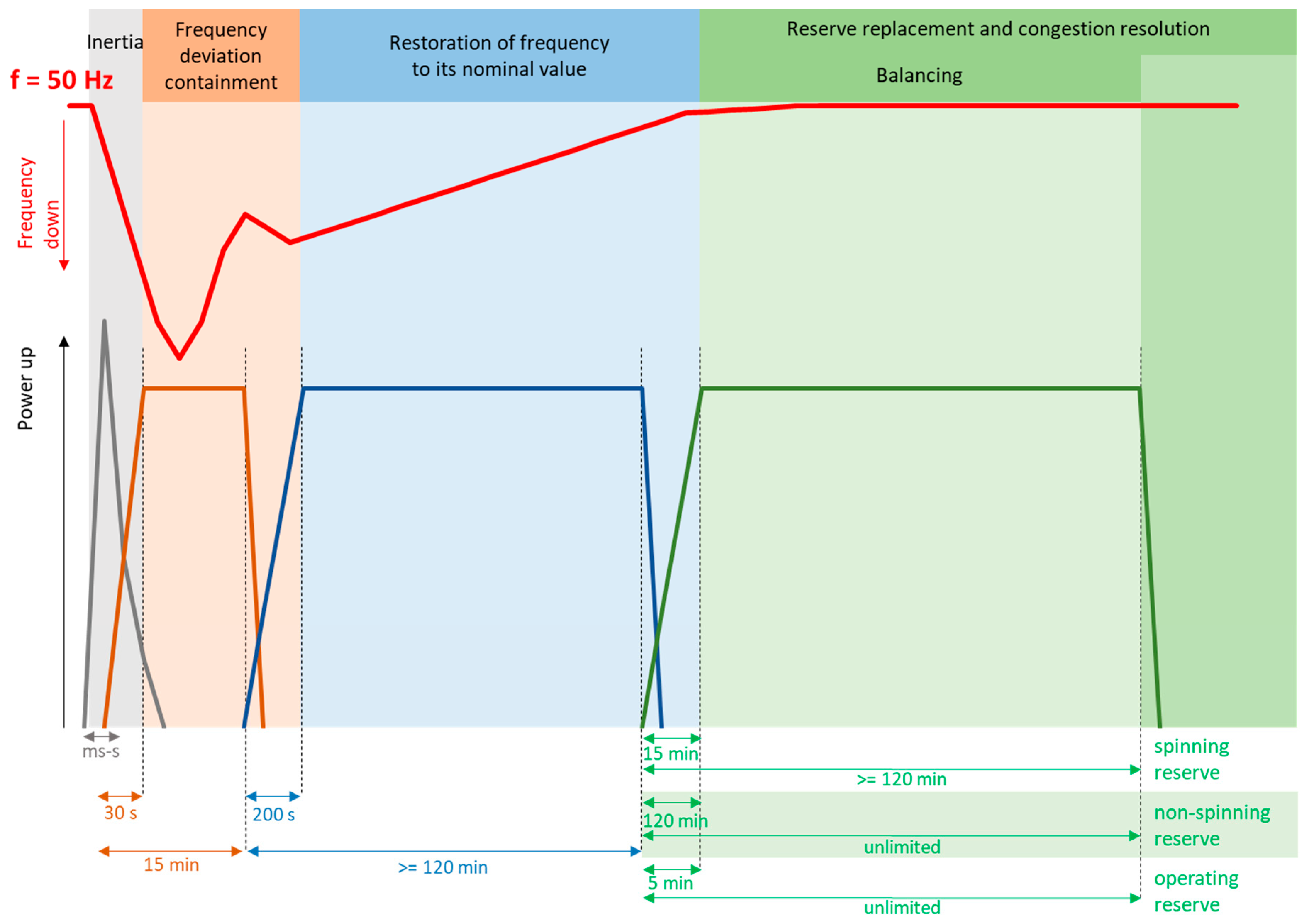
Load-frequency control, the creation of technical reserves, and the corresponding control performance are essential to allow for daily TSO operations [4,5]. Three main frequency-regulation reserves are defined on the European level, namely, the primary, secondary, and tertiary reserves; their transposition into national-market products is still heterogeneous among European Union (EU) states. Figure 1 presents their technical characteristics for the Italian network code, identifying the relevant activation time, the minimum required duration, and the main purpose.

Inertia (in grey) is related to synchronous machines connected to the power system and is associated to the kinetic energy of their rotating mass. Since renewable-energy plants, such as photovoltaic (PV) and wind, are connected to the grid by static converters or asynchronous generators, power system inertia is reduced, deteriorating grid stability. On the other hand, virtual inertia logics can be implemented in electronic-power-based systems [6].

Primary control is the fastest regulation (light brown line) aiming at stabilizing the frequency value; in Italy, it is automatically and locally activated for every programmable significant unit (i.e., with a nominal power greater than 10 MVA). Its required volume is defined on the basis of ENTSO-E prescriptions with respect to the so-called “reference incident”, where a contemporary loss of 3000 MW of generation is assumed on the EU level. The reserve needed from the Italian control area is evaluated by multiplying the total EU need by a contribution coefficient [7]. This coefficient reflects the weight of each control area on the overall synchronous area [8]. Its computation is based on the ratio between the yearly sum of energy produced and consumed in the Italian control area with respect to the sum of production and consumption of continental Europe (equal to 10.4% as per 2018 data [9]).

Secondary and tertiary controls (in blue and green, respectively) are activated in a subsequent moment, aiming at bringing the frequency back to its nominal value and coping with possible future frequency-variation events.

The SO GL prescribes to estimate reserve requirements following both a deterministic and a probabilistic approach [3]. The deterministic approach is mainly in use for the secondary reserve or automatic frequency restoration reserve (aFRR): it is also known as the empirical noise method, and it expresses reserve requirements as a function of maximal peak load in a region [10]. The probabilistic approach is detailed in [11], where the input variables for sizing (i.e., power plant outages, load variation, forecast errors and exchange schedules) are listed and explained as well as the reasons for adopting a probability density function (thus, a statistical or probabilistic approach). This is adopted in many cases for sizing the tertiary reserve or manual frequency restoration reserve (mFRR).

Internationally, there are different techniques for sizing the reserve resources. In [12], after estimating aFRR requirements for some countries following the empirical noise method [13], the minimal contracted aFRR for 2010 in the same countries is shown. The contracted aFRR is usually comparable with the requirement (with some exceptions, e.g., in Switzerland, where the contracted reserve is largely above the requirement). Similarly, in Germany, the contracted aFRR is much higher than the requirement [14]; this can be due to the fact that German TSOs use a probabilistic method based on the statistical convolution of stochastic variables that considers a very high confidence interval (99.95%), resulting in a high level of security [10]. On the other hand, in Belgium, the contracted aFRR is smaller than the requirement in the guidelines. These different TSOs’ sensibilities result in widely varying amounts of aFRR and mFRR for different countries in the Continental Europe Synchronous Area, ranging from 5% to 15% of maximal peak load [10].

Some measures can be adopted to efficiently cover the control needs, and some improvements are proposed in the literature and by TSOs to decrease the total amount of reserve. For instance, in [12], the effect of two TSO cooperation concepts on aFRR sizing was proposed: the possibility of decreasing the total aFRR contracted by developing larger LFC blocks and by cooperation among TSOs was investigated. The sizing of aFRR and mFRR against different product lengths was investigated in [15], showing that larger product lengths imply larger reserves. In [14], the Belgian TSO proposed a new methodology for aFRR sizing: an improved probabilistic approach investigated (in 2020) in a proof of concept. Results of the TSO’s study showed that an improvement in estimation techniques (e.g., the use of calibrated machine-learning techniques) could lead to a decrease in reserve sizing. The same effect can be obtained by considering more relevant variables in the computation: for instance, the impact of the International Grid Control Cooperation (IGCC) on reserve needs, whose aim is exactly to perform the imbalance netting of aFRR among European countries.

This work develops a methodology to size secondary and tertiary reserves, corresponding to aFRR, mFRR, and replacement reserve (RR) products introduced by SO GL [3]. For the sake of clarity and brevity, the procedure is illustrated focusing on the bidding zone of northern Italy. Moreover, the methodology was built following indications provided by Annex 22 of Terna’s Network Code [16], which specifies that the calculation of balancing reserve needs is performed over aggregates of geographical zones; these aggregates are:

• Continente, which includes the entire Italian peninsula;
• Sicilia and Sardegna (geographical islands connected to the Italian peninsula thanks to AC and HVDC links) bidding zones, when their connection capacity with aggregate Continente is not high enough to prevent any balancing reserve shortage.

Collected data refer to 2017, 2018, and 2019, and concern the consumption and production of electricity; moreover, to evaluate the uncertainty linked both to loads and NP-RES; data about electricity-consumption and -production forecasts were also gathered.

Results are presented showing the calculated reserve-duration curve for the analyzed period, the standard forecast error derived from the collected data for load, wind, and solar energy, and all other elaborated parameters during the described procedure. After introducing a methodology for all the three reserves cited above, results are compared to Italian market data; however, this comparison does not seem significant due to the low degree of transparency currently characterizing the actions performed by Terna on the balancing market, where it acts as a unique, central counterpart. Despite this, the methodology shows good potential for further improvement, both updating it thanks to new data and by applying it to different control areas.

The remainder of the paper is organized as follows. Section 2 and Section 3 describe the methodology elaborated for secondary and tertiary spinning reserve evaluation, respectively. Section 4 details the procedure for the tertiary nonspinning reserve, focusing on the diverse terms contributing to its definition. Lastly, Section 5 briefly compares the obtained results with data elaborated from the Italian market, and draws some general conclusions.

2. Calculation of Secondary (aFRR)-Reserve Need

The calculation of the secondary reserve need is based on the ENTSO-E methodology described in [13], and particularly on the empirical reserve-sizing approach aimed at the noise management defined in Section B, Definition 5.1. The recommended minimal amount of secondary control reserve (aFRR) of a control area can be calculated as

$$\mathrm{aFRR}=\sqrt{{\mathrm{a}\ast \mathrm{L}}_{\mathrm{MAX}}{+\mathrm{b}}^2}-\mathrm{b},$$

(1)

where L_MAX is the maximal forecasted load for the control area, and a and b are equal to 10 and 150 MW, respectively. Annex 22 of the Italian NC specifies that aFRR need should be defined hourly per each aggregate of the geographical zones, resulting in being a function of the forecasted hourly load of the same aggregate. Moreover, the secondary reserve is symmetrically defined for upward and downward regulation.

Data of the day-ahead forecast and actual load for the Continente aggregate were downloaded from the ENTSO-E Transparency Platform for 2017, 2018, and 2019 [17], and the above formula was applied to such data in order to compute the hourly secondary-reserve need. Figure 2 shows the mean value for the aFRR need that was calculated, grouped by hour of the day and day of the week for each of the three analyzed years. The profiles for the different years are very similar, showing a higher reserve need for working days than that for holidays, and reflecting the different load levels along the week (for the scope of calculations reported in Figure 1, national holidays were classified as Sundays).

3. Calculation of Spinning (mFRR)-Tertiary-Reserve Need

The spinning tertiary reserve is associated to the manual FRR as defined in the SO GL and to tertiary regulation “pronta” of the Terna network code. The spinning and nonspinning tertiary reserves define the total tertiary reserve. According to Annex 22 of the Terna network code, spinning reserve need is calculated only for upward regulation, for each aggregate of geographical zones, in order to cope with

• the full replacement of secondary-reserve needs for the same aggregate;
• the temporal advance or delay of residual load ramps with respect to the forecasted behavior, where residual load is defined as the gross load minus PV power-plant injection and energy exchanges with bordering foreign bidding zones.

Moreover, Annex 22 specifies that the spinning-reserve need for the northern Italy bidding zone must be considered to be equal to the spinning-reserve need for the aggregated Continente area.

Because of this, the residual load in the northern Italy area (the study case adopted in this paper) was computed as the difference between the forecasted load of the Continente area and:

• the total forecasted PV production in the four bidding zones belonging to the aggregate Continente;
• the commercial energy exchange with the foreign zones, taken positive if the power flows from Italy to another state, negative if vice versa.

On this basis, considering data gathered for 2017, 2018 and 2019, the hourly spinning-reserve need of the northern Italy bidding zone was calculated as:

$${\mathrm{mFRR}}_{\mathrm{spin}}^{\mathrm{North}}{=\mathrm{aFRR}}^{\mathrm{Continente}}\ast \left(1+\left|{\mathrm{LoadRamp}}^{\mathrm{Continente}}\right|\right),$$

(2)

where aFRR is computed as specified above, while load ramp contribution is defined as:

$${\mathrm{LoadRamp}}^{\mathrm{Continente}}=\frac{{\mathrm{ResidualLoad}}_{\mathrm{i}}^{\mathrm{Continente}}{-\mathrm{ResidualLoad}}_{\mathrm{i}-1}^{\mathrm{Continente}}}{{\mathrm{ResidualLoad}}_{\mathrm{i}}^{\mathrm{Continente}}}$$

(3)

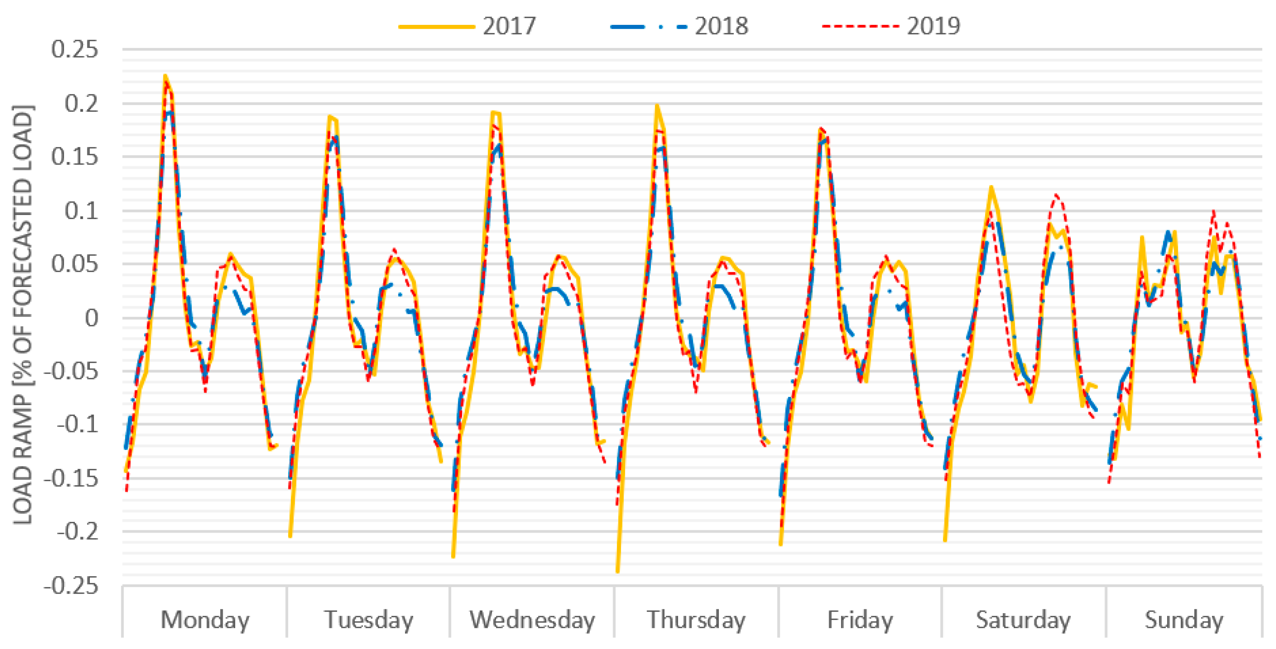
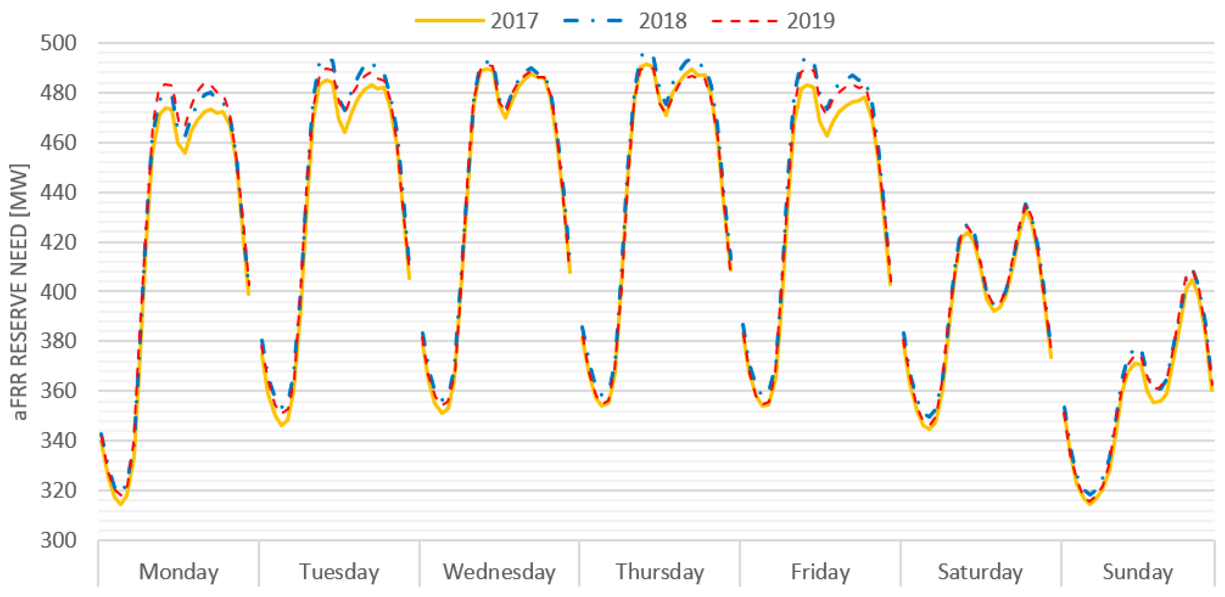
for every hour i of the three considered years. The load-ramp contribution is, thereby, calculated as the absolute value of the residual-load variation foreseen between one hour and the previous one, expressed as a percentage of the forecasted residual-load value for the same hour. Figure 3 presents the mean value of the load ramp calculated on the Continente area for the analyzed years; in this case, it is also possible to see homogeneity among 2017, 2018, and 2019 data, beyond a similar behavior among different days of the week.

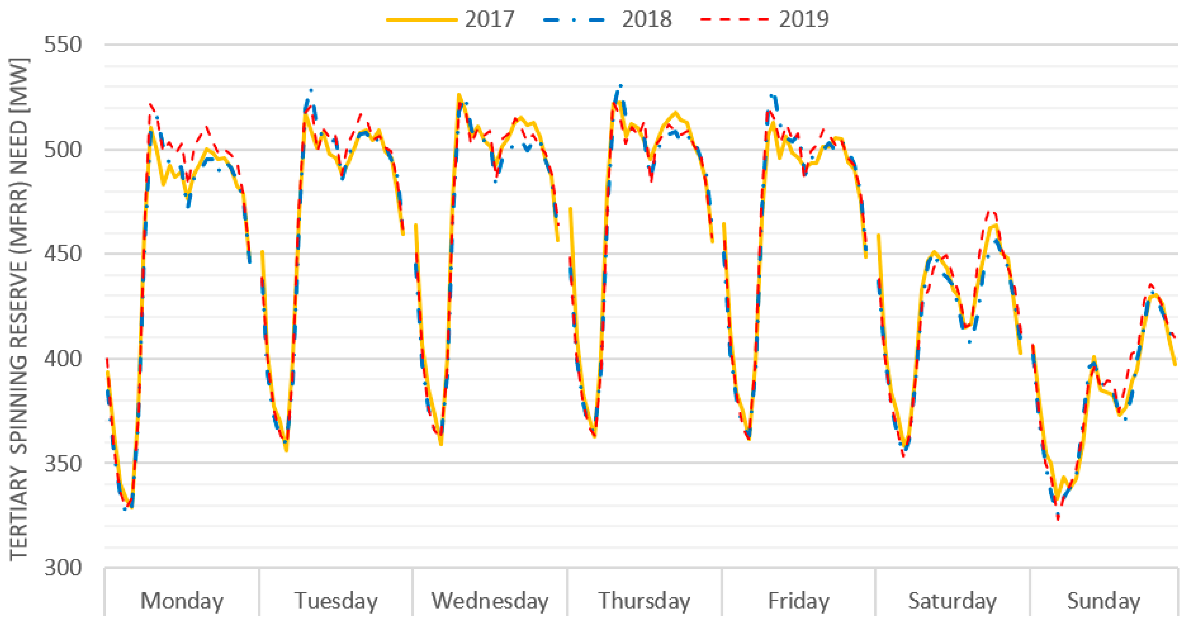
Figure 4 presents the mean value for the spinning tertiary reserve over the analyzed period, showing similar behavior to the ones depicted above, confirming that there is a strong link between spinning reserve (hence electric load), hour of the day, and day of the week; moreover, the required spinning reserve was substantially constant along the studied time interval. Tertiary spinning reserve is only defined, as stated above, for upward reserve need.

4. Calculation of Nonspinning-Tertiary-Reserve (RR) Needs

Annex 22 of the Italian network code defines the hourly need for upward nonspinning tertiary reserve for each bidding zone as the statistical combination of:

• nonprogrammed unavailability of a thermoelectric-power plant having the maximal value in the final binding injection program, increased by its upward reserved quantity;
• error in the forecast of the load and of nonprogrammable power-plant production, evaluated with a confidence interval of 99.7%, under the hypothesis that errors are independent of each other;
• a loss of production from power plants under trial.

Similarly, concerning downward regulation, nonspinning-tertiary-reserve need calculation is based on a combination of:

• nonprogrammed unavailability for a hydroelectric pumping power plant with a maximal value for the final binding withdrawal program, increased by its downward reserved quantity;
• error in the forecast of the load and of nonprogrammable power-plant production, evaluated with a confidence interval of 99.7%, under the hypothesis that errors are independent of each other.

On the basis of these considerations, the nonspinning upward and downward reserve needs were calculated as:

$${\mathrm{RR}}_{\mathrm{Nspin},\mathrm{upward}}^{\mathrm{North}}{=\mathrm{P}}_{\mathrm{MAX},\mathrm{thermo}}^{\mathrm{Continente}}+2.74\ast \sqrt{{\mathsf{\sigma }}_{\mathrm{LOAD}}^2{+\mathsf{\sigma }}_{\mathrm{WIND}}^2{+\mathsf{\sigma }}_{\mathrm{PV}}^2}$$

(4)

$${\mathrm{RR}}_{\mathrm{Nspin},\mathrm{downward}}^{\mathrm{North}}{=\mathrm{P}}_{\mathrm{MAX},\mathrm{pumped}}^{\mathrm{Continente}}+2.74\ast \sqrt{{\mathsf{\sigma }}_{\mathrm{LOAD}}^2{+\mathsf{\sigma }}_{\mathrm{WIND}}^2{+\mathsf{\sigma }}_{\mathrm{PV}}^2},$$

(5)

where the contribution of on-trial power plants to the upward reserve need was neglected. The next subsections describe the procedure followed to compute each term of the above formula.

4.1. Contribution from Thermoelectric- and Hydroelectic-Power-Plant Binding Programs

To evaluate the contribution coming from thermoelectric and hydroelectric power plants to the upward and downward tertiary-nonspinning-reserve needs, data coming from different electricity markets were exploited. In particular, considering 2017, 2018, and 2019, data from day-ahead market (DAM), intraday market (IDM) and ancillary-services market (ASM) sessions, available at [18], were downloaded. These data allowed for assessing the binding injection or withdrawal program specific to each power unit for every hour of analyzed the period.

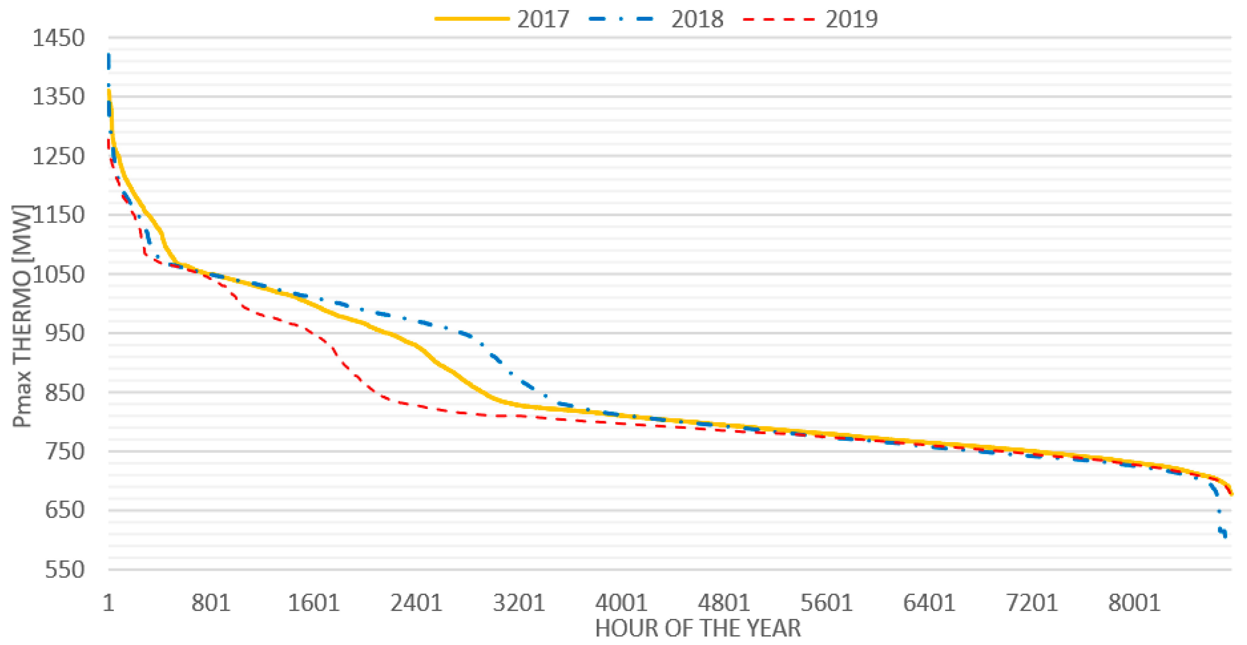
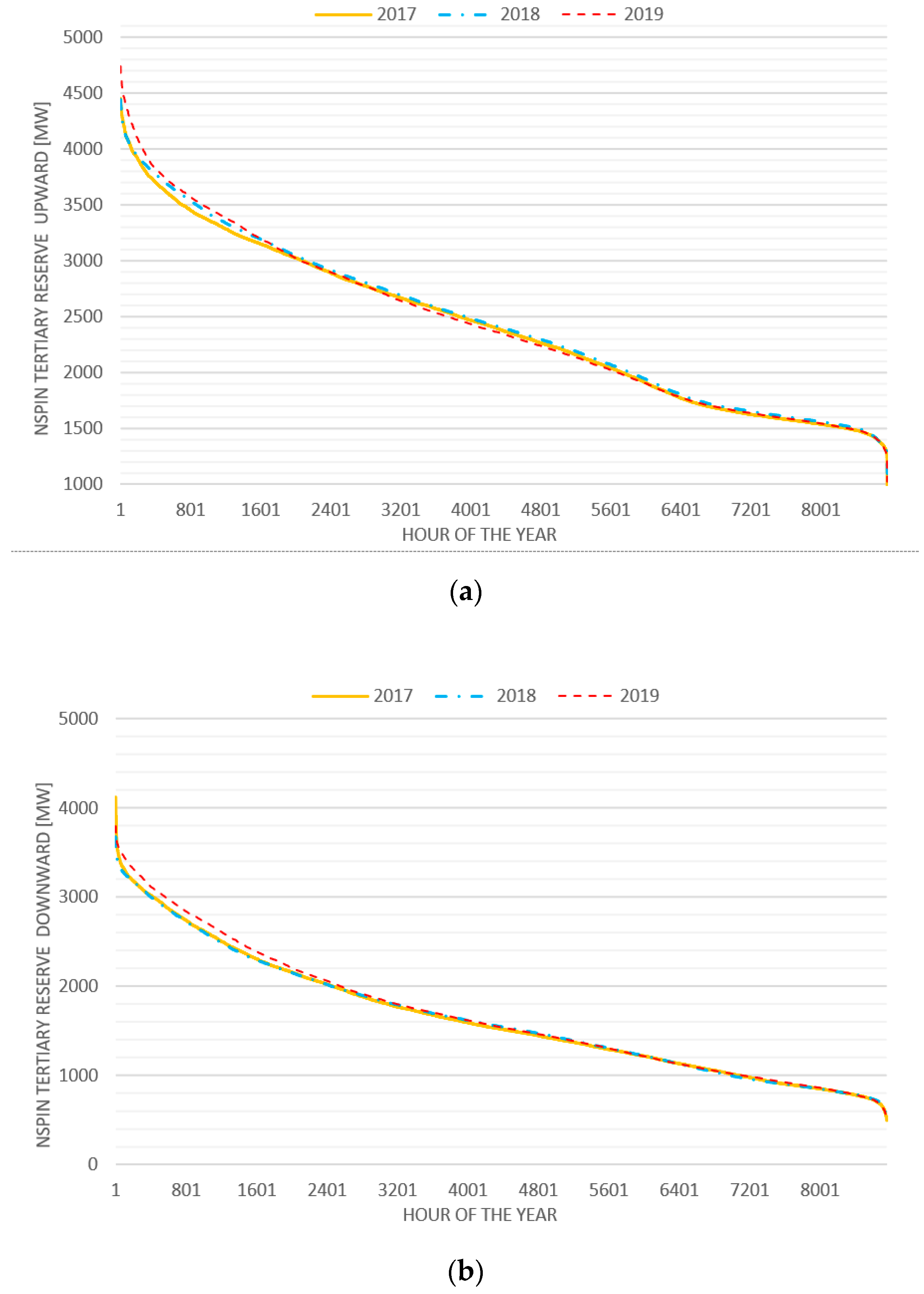
For thermoelectric-power units, the injection binding program was summed up with the upward regulation capacity available from the same unit; among all thermoelectric units over the geographical area defined by the Continente aggregate, the one for which this summation was at the maximum was chosen, and the summation value was considered for upward nonspinning reserve computation. Figure 5 presents the duration curve of this term along the analyzed time period.

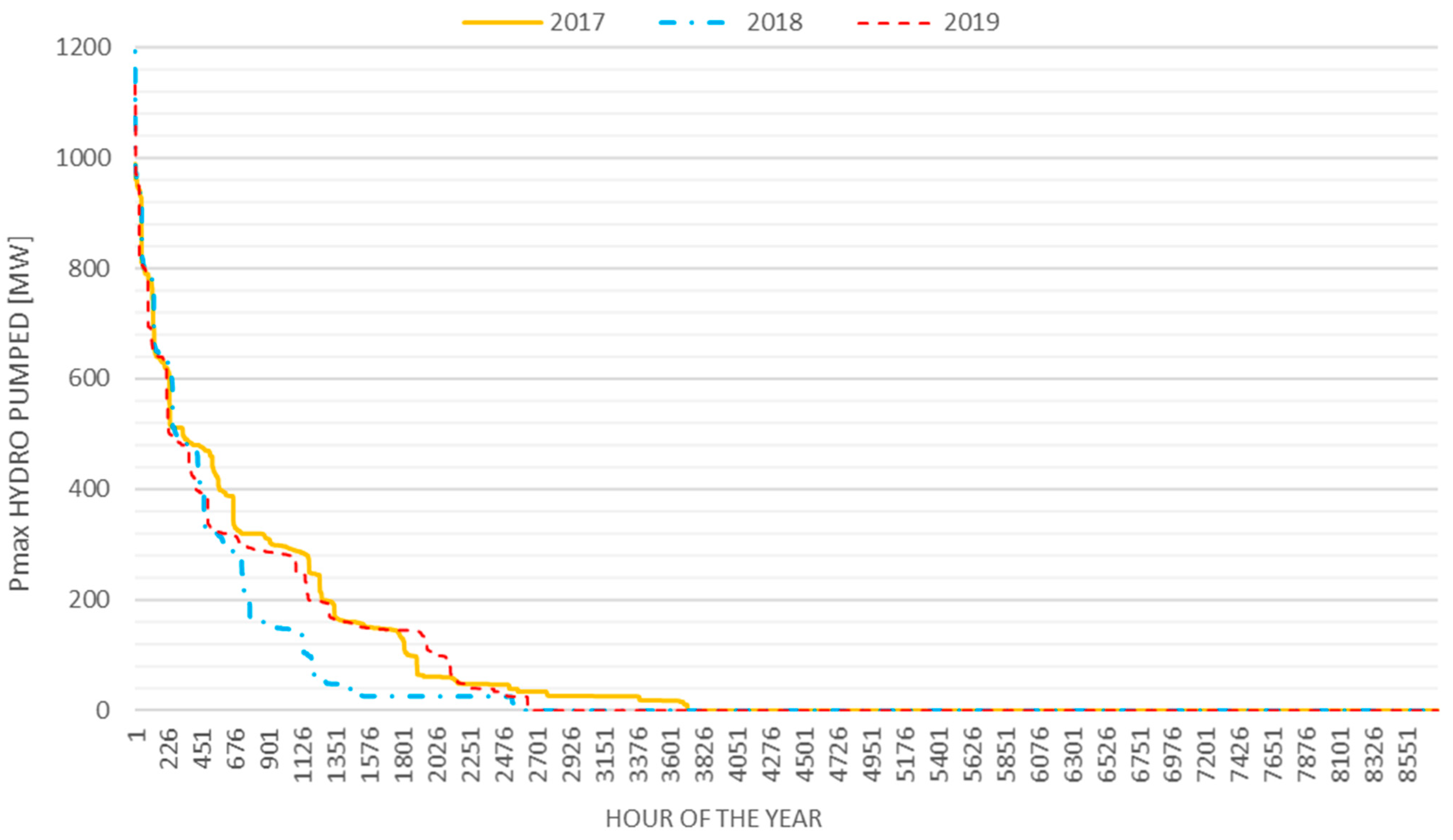
A similar procedure was also exploited for hydroelectric pumping power units, for which the binding withdrawal program was summed to the downward regulation capacity available for the same unit. Among all hydroelectric units over the geographical area defined by the Continente aggregate, the one for which this summation was maximal was chosen, and its value was considered for the downward nonspinning reserve computation. Figure 6 presents the duration curve of this term along the analyzed time period.

4.2. Contribution from Load-Forecast Error

In order to evaluate the contribution of load forecast error to the nonspinning reserve, the procedure adopted in [19] was considered. In particular, data for the forecasted and the actual load for the Continente aggregate were downloaded from the ENTSO-E Transparency Platform, and the hourly load forecast error was computed as

$${\mathrm{E}}_{\mathrm{load}}[\%]=\frac{{\mathrm{ActualLoad}}_{\mathrm{i}}^{\mathrm{Continente}} {-\mathrm{ForecastLoad}}_{\mathrm{i}}^{\mathrm{Continente}}}{{\mathrm{ForecastLoad}}_{\mathrm{i}}^{\mathrm{Continente}}},$$

(6)

where E_load is defined as a percentage of the forecasted load value. Data concerning the load forecast error for 2017, 2018, and 2019 were grouped by hour of day and day of week, and the standard deviation of the empirical distribution of the load forecast error obtained was calculated as

$${\mathsf{\sigma }}_{\mathrm{load}}^{(\mathrm{h},\mathrm{d})}[\%]=\sqrt{\frac{{{\displaystyle \sum }}_{\mathrm{N}}{\left({\mathrm{E}}_{\mathrm{load}}^{\mathrm{n}}{-\mathsf{\mu }}^{(\mathrm{h},\mathrm{d})}\right)}^2}{\mathrm{N}}},$$

(7)

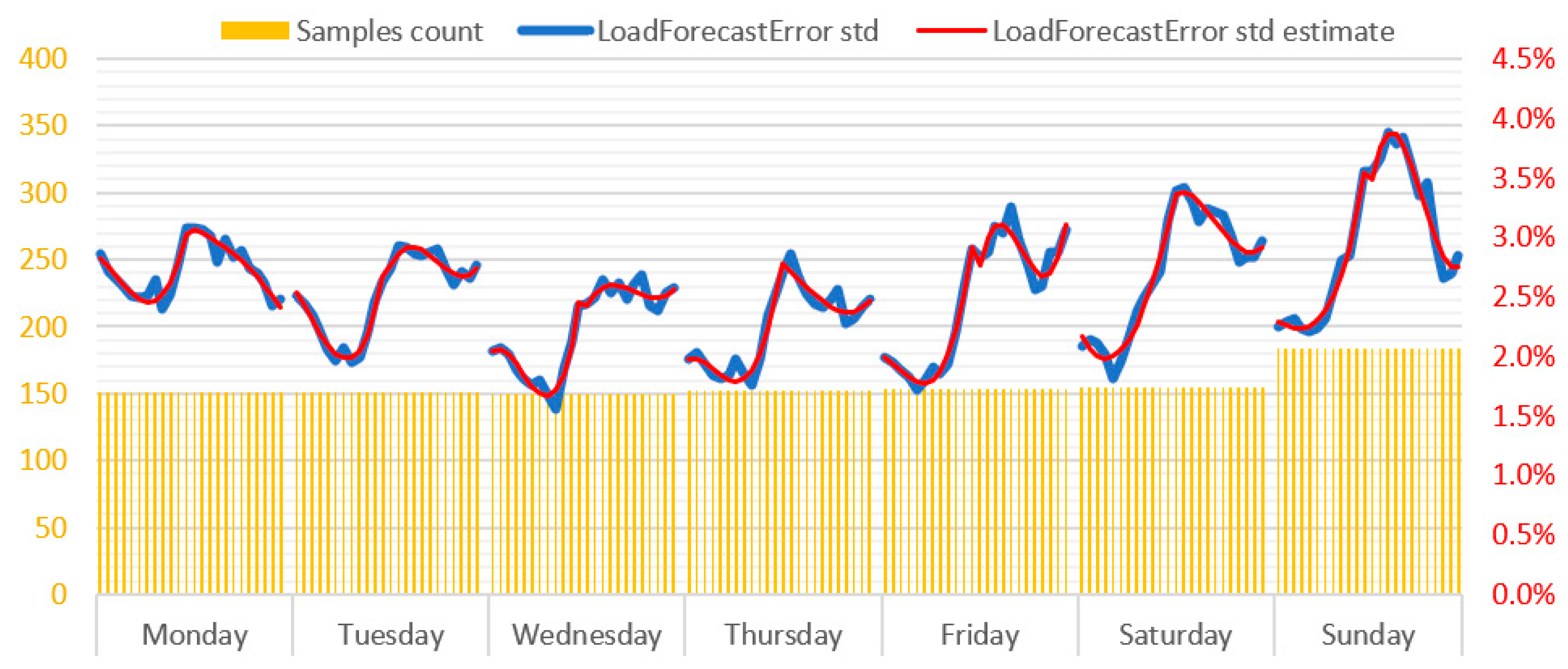
where (h,d) is an index that identifies a specific couple (hour,day), N is the total number of samples falling in set (h,d), and μ is the mean value of the error calculated for set (h,d). For the scope of this analysis, national holidays were classified as Sundays. Figure 7 presents the standard deviation of the load-forecast error calculated for each couple (hour,day); the left axis reports the number of available samples for each set (hour,day), while the right axis refers to the standard-deviation value. The blue curve represents the exact value calculated for the standard deviation, while the red curve is an approximation, i.e., data-driven regression adopted to point out the trend for the nonspinning-reserve need.

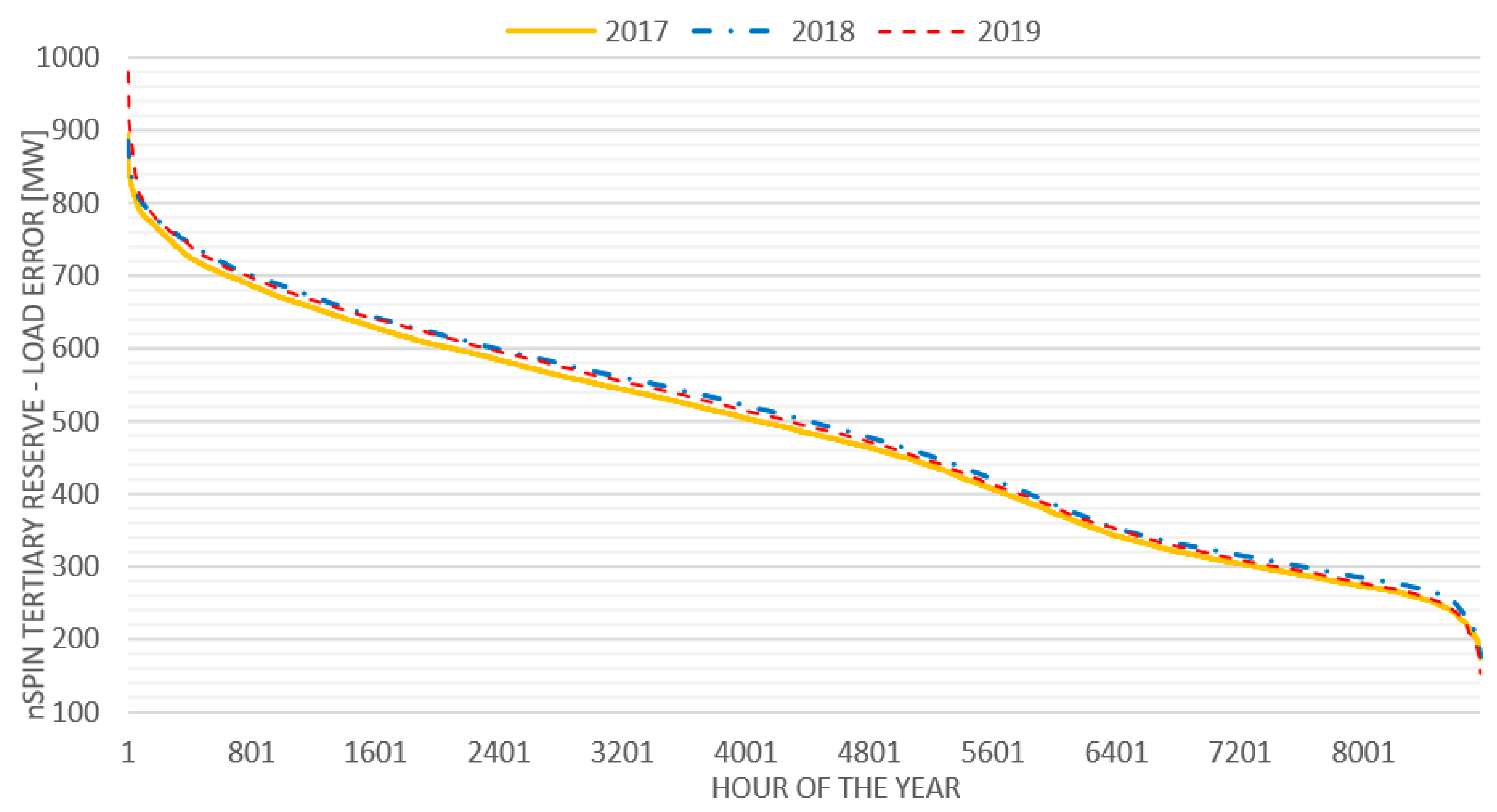
Lastly, the contribution of load-forecast error was converted into MW for each hour i of the t analyzed time period.

$${\mathsf{\sigma }}_{\mathrm{LOAD}}^{\mathrm{i}\in (\mathrm{h},\mathrm{d})}\left[\mathrm{MW}\right]{=\mathsf{\sigma }}_{\mathrm{load}}^{(\mathrm{h},\mathrm{d})}[\%]{\ast \mathrm{ForecastLoad}}_{\mathrm{i}}^{\mathrm{North}}\left[\mathrm{MW}\right]$$

(8)

Figure 8 presents the duration curve of the contribution to the needed amount of nonspinning tertiary reserve relevant to the load-forecast error in the northern zone.

4.3. Contribution from Wind-Production Forecast Error

Differently from the load forecast, wind-forecast error cannot be evaluated by grouping samples on the basis of the hour of the day and the day of the week. On the basis of the literature review and observations reported in [19], the standard deviation of the wind-forecast error showed dependence on two particular contingencies:

• the forecasted level of production that indirectly represents foreseen wind speed (expressed through σ¹_w), and
• the time horizon over which the forecast was issued (expressed through σ²_w).

In the proposed approach, two parallel analyses were carried out in order to associate distribution (and standard deviation) to the forecast error for both the above-listed conditions; lastly, a single value for the standard deviation was derived.

Data concerning actual and forecasted wind production were downloaded from the ENTSO-E Transparency Platform for 2017, 2018, and 2019 for aggregate Continente. According to the ENTSO-E platform, data for wind-forecast production were classified into:

• day-ahead forecast, which is communicated at 18:00 of the day before the delivery;
• intraday forecast, which is communicated at 08:00 of the delivery day; and
• last forecast, which is the last available value communicated by the TSO during the production day.

According to this information, and on the basis of the sequence of Italian market sessions, that data related to the last forecast were updated at 16:00 of the delivery day. Supporting the above statement, analysis of the available data showed that:

• day-ahead forecast is equal to the intraday forecast for every hour before 08:00 each day, and
• intraday forecast is equal to last forecast for every hour before 16:00 of each day.

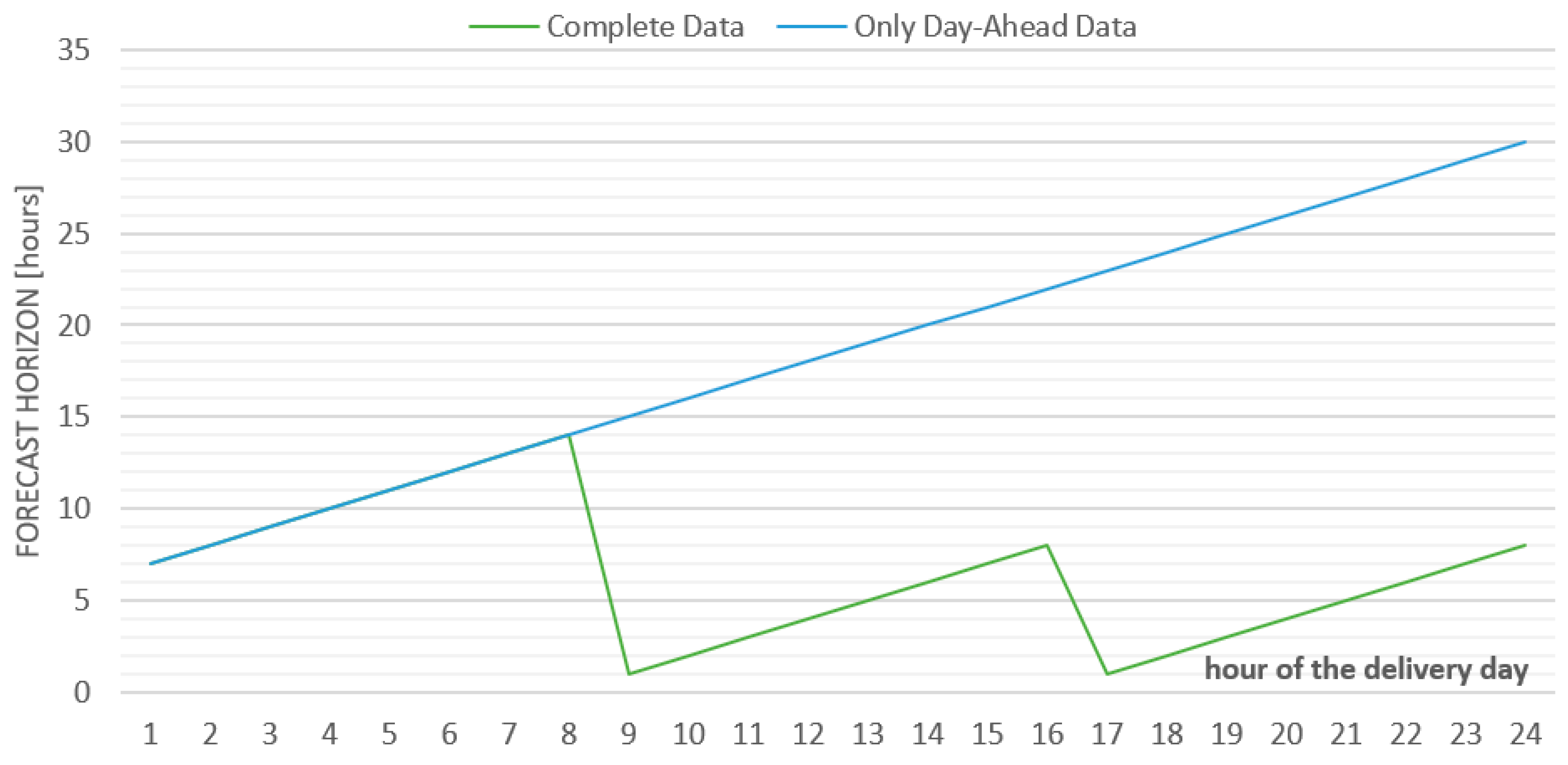
On this basis, it was possible to associate a forecast horizon to each datum, defined as the number of hours between the hour in which the forecast is updated and the hour to which the forecast refers. Moreover, for almost half of the collected data (from 2017 to half of 2018) only day-ahead forecasts were available; hence, the considered time horizon was fully referred to the day-ahead forecast time. Figure 9 reports the considered forecast horizon for complete data, where all three forecast updates were available, and for day-ahead data only, where only a day-ahead forecast was available.

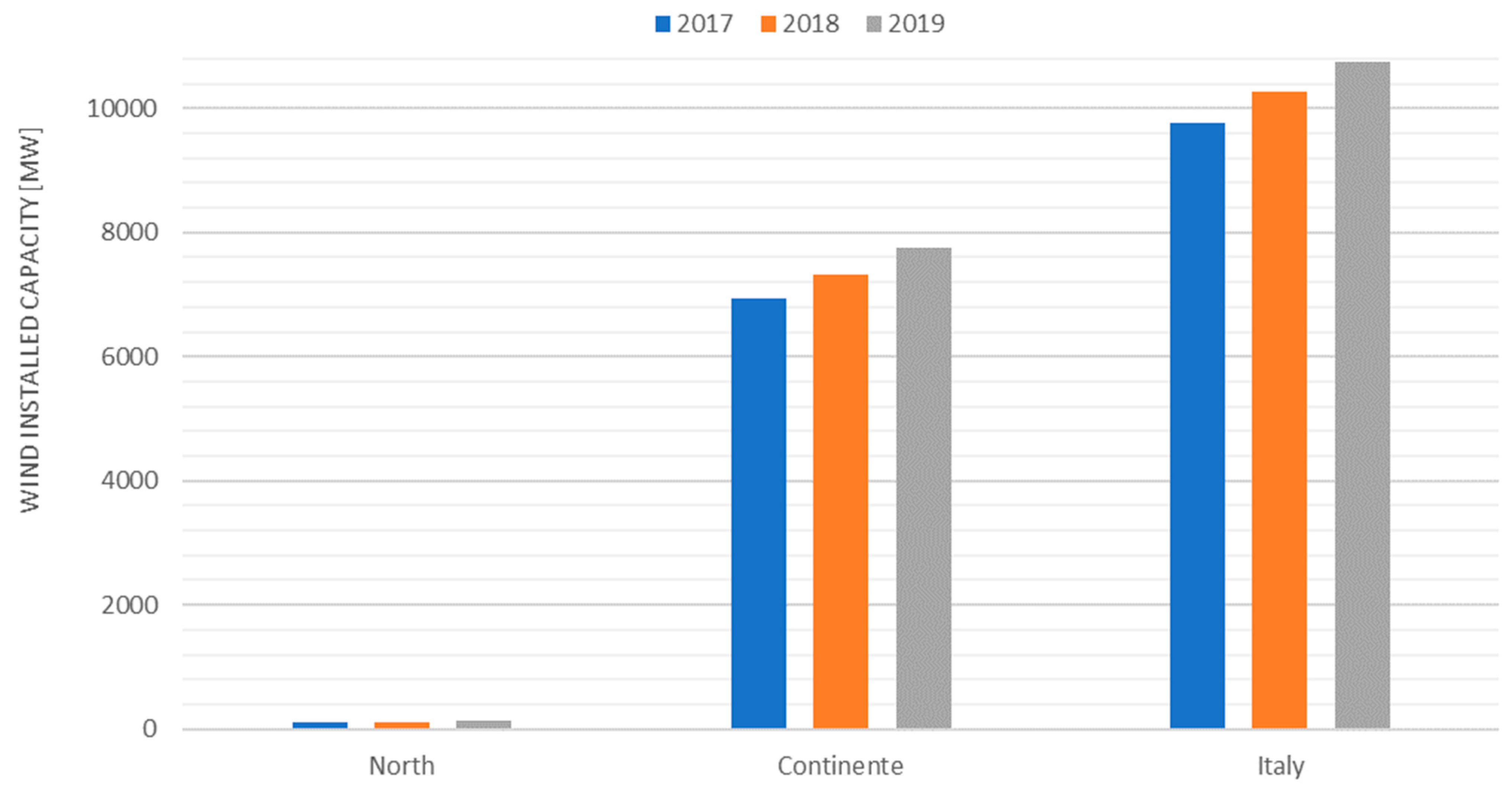
Beyond data concerning the wind-production forecast, data about installed wind capacity in Italy were also collected from [20,21]. Figure 10 presents these data on the analyzed time period, distinguishing between the northern bidding zone, the Continente aggregate, and Italy as a whole. As displayed, the northern zone hosts an almost negligible amount of wind plants (roughly 120 MW), while installed capacity is much higher in other bidding zones (up to 10 GW).

Starting from collected data for wind-forecast production and installed wind capacity, σ¹_w and σ²_w were computed as follows. First, wind-forecast error was calculated for every hour of the analyzed period (2017, 2018, and 2019) as:

$${\mathrm{E}}_{\mathrm{wind}}=\frac{{\mathrm{ActualProduction}}_{\mathrm{i}}^{\mathrm{Continente}}{-\mathrm{ForecastProduction}}_{\mathrm{i}}^{\mathrm{Continente}}}{{\mathrm{InstalledCapacity}}_{\mathrm{wind}}^{\mathrm{Continente}}}$$

(9)

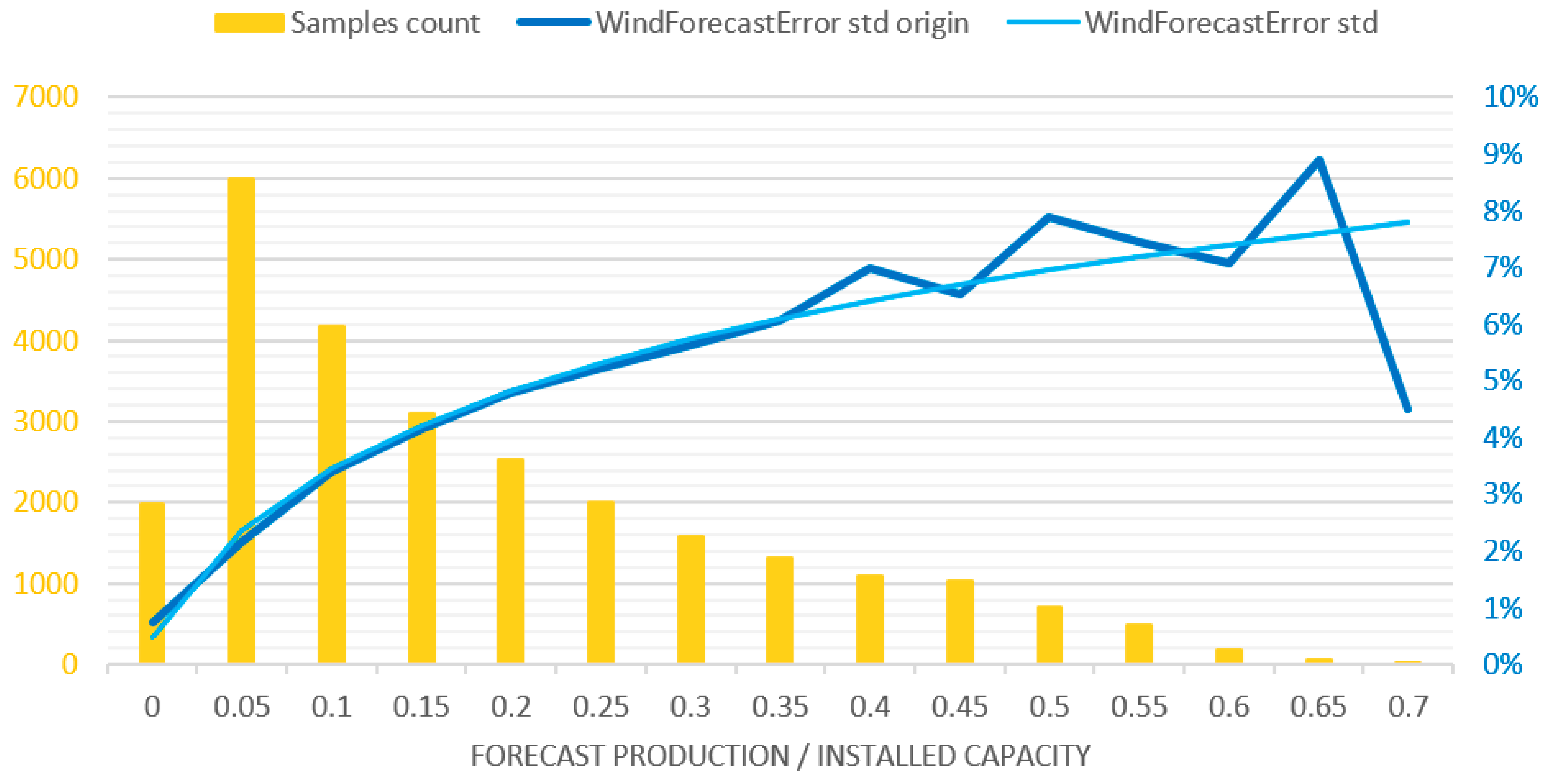
σ¹_w was calculated as the standard deviation of the wind-forecast error distribution, grouping it on the basis of the ratio between forecasted production (MW) and installed capacity (MW) in each and every hour.

$${\mathsf{\sigma }}_{\mathrm{w}}^{\mathrm{F}/\mathrm{I}}=\mathrm{f}\left(\frac{\mathrm{ForecastProduction}}{\mathrm{InstalledCapacity}}\right)$$

(10)

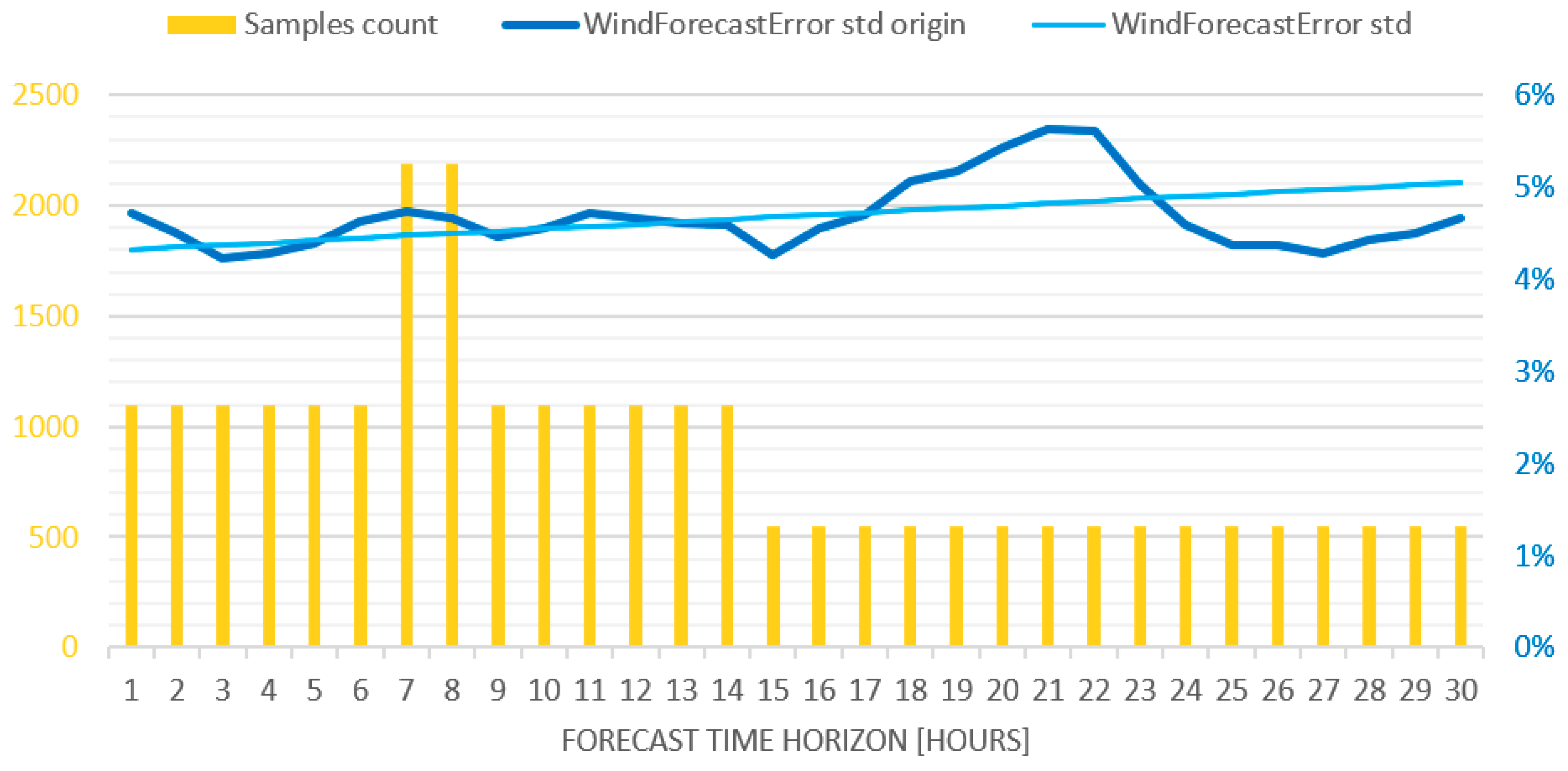
Figure 11 shows the obtained results. Yellow, referred to in the left y axis, reports the number of available samples for each x-axis interval; blue, referred to in the right y axis, presents the calculated value for the forecast-error standard deviation; light blue reports the actual approximation used for nonspinning-reserve calculation. Uncertainty linked to wind-forecast production considerably increase with forecast production itself, showing strong dependence on the wind-speed value.

Moreover, σ²_w was calculated as the standard deviation of wind-forecast error distribution, grouping it on the basis of the forecast time horizon.

$${\mathsf{\sigma }}_{\mathrm{w}}^{\mathrm{FTH}}=\mathrm{f}\left(\mathrm{ForecastTimeHorizon}\right)$$

(11)

Figure 12 shows the results of this analysis, reporting the number of samples available in yellow, the computed standard-deviation value in blue, and the used approximation in the following calculations in light blue. Data confirmed correlation between forecast uncertainty and forecast time horizon, even if this dependence was weaker than the one shown for σ¹_w.

The two aspects, represented by σ¹_w and σ²_w, can be merged by calculating the standard deviation of the combined distribution, supposing that the two errors are independent.

$${\mathsf{\sigma }}_{\mathrm{wind}}^{\left(\frac{\mathrm{F}}{\mathrm{I}};\mathrm{FTH}\right)}[\%]=\sqrt{{\mathsf{\sigma }}_{\mathrm{w}}^{F/I }{}^2{-\mathsf{\sigma }}_{\mathrm{w}}^{\mathrm{FTH}}{}^2}$$

(12)

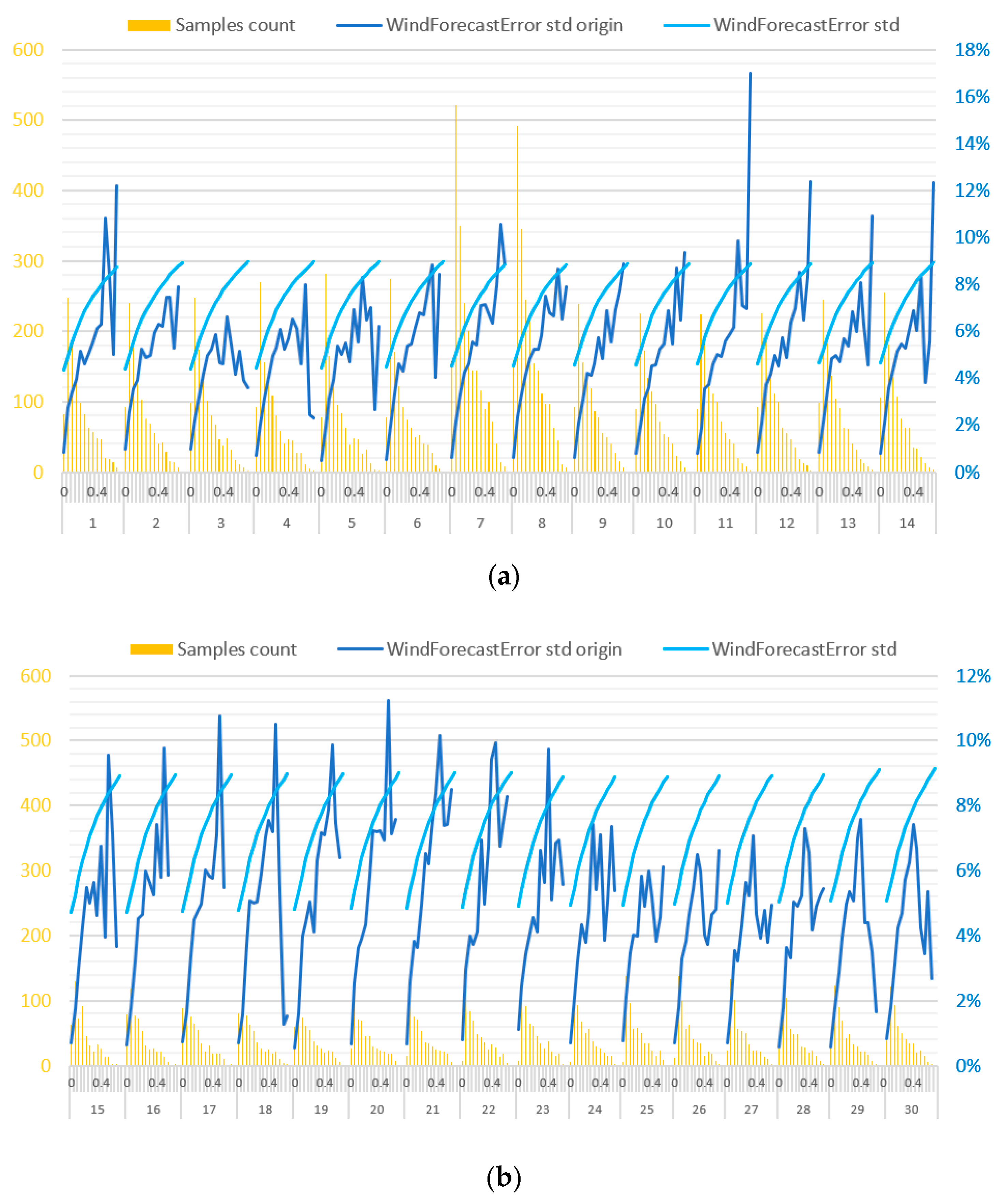
The final standard deviation of the wind-forecast error thereby depends on both the forecast time horizon (FTH, first reference x axis) and the forecast production level (F/I, second reference x axis). Figure 13a,b show the obtained results for this analysis. While there is strong dependence on the forecasted production level, uncertainty linked to wind forecast remained stable or slightly increased among the different forecast time horizons. In particular, Figure 13a presents data concerning a forecast time horizon up to 14 h before the delivery hour, and Figure 13b presents data concerning a forecast time horizon from 15 to 30 h before the delivery hour. Gathered data refer to 2017, 2018, and 2019.

Lastly, the wind-forecast standard error expressed in MW was calculated on the basis of the previously defined standard deviation and the installed wind capacity in the northern zone. Hence, this error depends on the ratio between forecast production and installed capacity, and on the forecast time horizon, as they were defined for each and every hour.

$${\mathsf{\sigma }}_{\mathrm{WIND}}^{\mathrm{i}\in \left(\frac{\mathrm{F}}{\mathrm{I}};\mathrm{FTH}\right)}{\left[\mathrm{MW}\right]=\mathsf{\sigma }}_{\mathrm{wind}}^{\left(\frac{\mathrm{F}}{\mathrm{I}};\mathrm{FTH}\right)}{[\%]\ast \mathrm{WindInstalledCapacity}}_{\mathrm{year}}^{\mathrm{North}}\left[\mathrm{MW}\right]$$

(13)

The computed value was corrected, as suggested in [19], considering that the downward standard deviation should be lower than 2/3 (i.e., 68% of possible situations in normal Gaussian distribution) of the forecast production, and that the upward standard deviation should be lower than 2/3 of the difference between installed capacity and forecast production. Figure 14a,b show the duration curve for the wind-related forecast error contributing to nonspinning-reserve calculation for upward and downward regulation, respectively; data are related to the northern bidding zone.

4.4. Contribution from Solar-Production Forecast Error

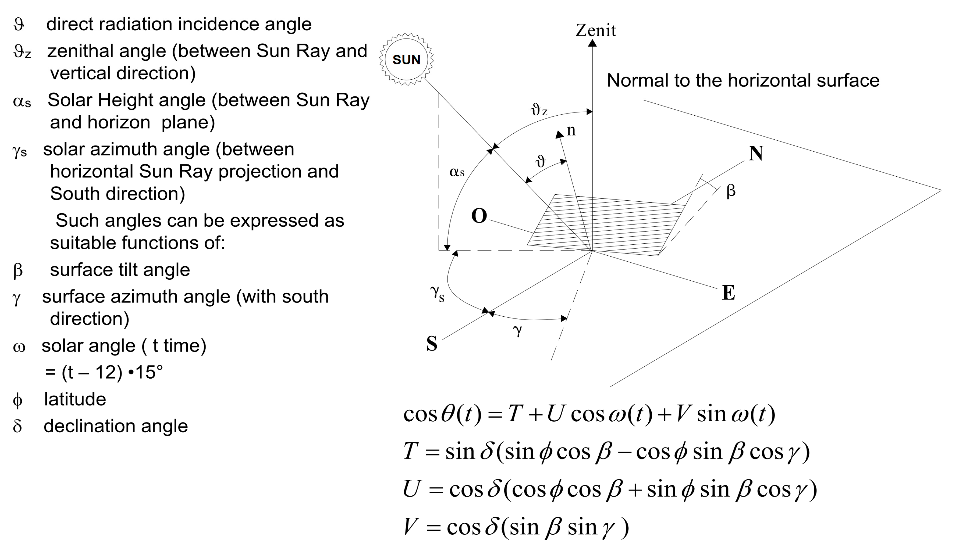
The literature review reported in [19] clearly indicated that the solar forecast error depends on the uncertainty linked to sky conditions; this issue is expressed in the scientific literature through the clearness index (CI), an index varying from 0 to 1 where the former defines a completely cloudy sky and the latter a fully sunny sky. The CI value can be calculated as the ratio between forecasted PV production and the maximal theoretical PV production available in each hour of the year. The latter can be computed through specific solar-related equations. Because of this, the first part of this subsection shows how maximal PV production was computed.

Considering the position of the sun in the sky, the angle shown in Figure 15 can be selected.

For the sake of simplicity, azimuth and tilt angle (γ and β, respectively) were set to zero, supposing a perfect exposition of PV panels to the south, and no inclination with respect to the horizontal plane. This introduced a bias in the results that was fixed in a second step, as detailed in the following. In particular, regarding the model’s parameters:

• latitude (ϕ) was set to 43.5° for centre-north, 41.5° for centre-south, 40° for south, and 45° for north;
• declination angle, which depends on the day of the considered year, was computed as

$$\mathsf{\delta }=23.45\ast \sin \left(360\ast \frac{284+\mathrm{n}}{365}\right),$$

(14)

where n is the progressive number of the day during the year,

• the solar angle was calculated as:

$$\begin{gathered} {\mathsf{\omega }=\mathrm{t}}_{\mathrm{s}}\ast 15°-202.5°\mathrm{if}\mathrm{in}\mathrm{Central}\mathrm{European}\mathrm{Time}; \\ {\mathsf{\omega }=\mathrm{t}}_{\mathrm{s}}\ast 15°-187.5°\mathrm{if}\mathrm{in}\mathrm{Central}\mathrm{European}\mathrm{Solar}\mathrm{Time} \end{gathered}$$

(15)

where solar time t_s is defined as:

$${\mathrm{t}}_{\mathrm{s}}\left[\mathrm{hour}\right]=\mathrm{h}+\frac{\left({4\ast \mathsf{\lambda }}_{\mathrm{loc}}{-\mathsf{\lambda }}_{\mathrm{standard}}\right)+\mathrm{E}\left(\mathrm{n}\right)}{60},$$

(16)

where h is the standard local time; λ_loc and λ_standard are the mean longitude of each zone and the longitude difference with respect to the Greenwich meridian, respectively; and E(n) is the Ephemerid or time equation expression. In particular, the Ephemerid is computed as:

$$\mathrm{E}\left(\mathrm{n}\right)\left[\mathrm{minutes}\right]=229.2\ast \left(\begin{array}{c}0.0000075+0.001868\ast \cos \left(\mathrm{B}\right)-0.03277\ast \sin \left(\mathrm{B}\right)\\ -0.014615\ast \cos \left(2\mathrm{B}\right)-0.0408\ast \sin \left(2\mathrm{B}\right)\end{array}\right)$$

(17)

where

$$\mathrm{B}=\left(\mathrm{n}-1\right)\ast \frac{360}{365}.$$

(18)

From the Ephemerid, it is possible to define the time correction factor (TCF) as

$$\mathrm{TCF}\left[\mathrm{minutes}\right]=\left({4\ast \mathsf{\lambda }}_{\mathrm{loc}}{-\mathsf{\lambda }}_{\mathrm{standard}}\right)+\mathrm{E}\left(\mathrm{n}\right).$$

(19)

Hence, solar local time is

$${\mathrm{t}}_{\mathrm{s}}\left[\mathrm{hours}\right]=\mathrm{local}\mathrm{time}+\frac{\mathrm{TCF}}{60}.$$

(20)

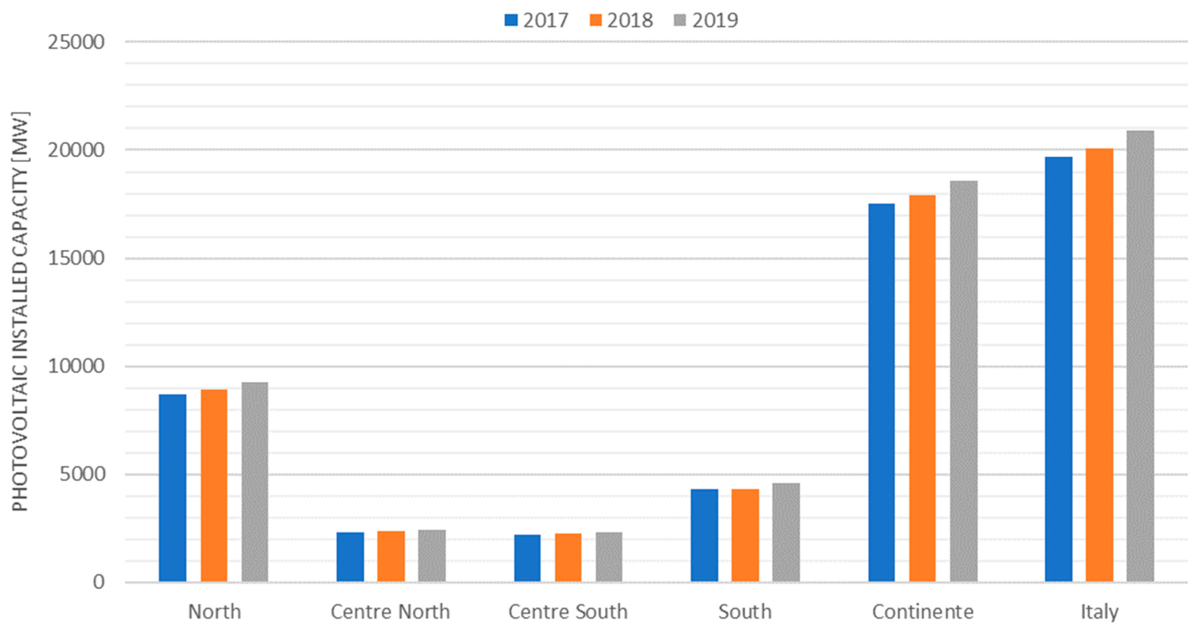
From the defined parameters above, the maximal PV production of each hour of the year can be calculated as

$${\mathrm{P}}_{\mathrm{PV},\mathrm{i}}^{\mathrm{MAX}}=\sin \left(\mathsf{\alpha }\right){\ast \mathrm{P}}_{\mathrm{PV}}^{\mathrm{INSTALLED}},$$

(21)

where α is the solar height, sin(α) = cos(θ), calculated as above, and installed PV capacity for each bidding zone for the Continente aggregate was taken from [20,21]; relevant data are detailed in Figure 16.

Data concerning the PV production forecast were downloaded from the ENTSO-E Transparency Platform, with the same structure described for the wind-forecast data. For the purpose of calculations, the most recent PV production forecast available in each hour of the analyzed time period (2017, 2018 and 2019) was considered. From the available forecasted PV production, the standard deviation of the distribution of the PV production forecast error was calculated as a function of the ratio between forecasted PV production and maximal theoretical production according to the position of the sun, computed for every zone as explained above.

Hence, solar-forecast error was calculated for each bidding zone as

$${\mathrm{E}}_{\mathrm{solar}}=\frac{{\mathrm{ActualProduction}}_{\mathrm{i}}^{\mathrm{Zone}}{-\mathrm{ForecastProduction}}_{\mathrm{i}}^{\mathrm{Zone}}}{{\mathrm{P}}_{\mathrm{PV},\mathrm{i}}^{\mathrm{MAX}}}$$

(22)

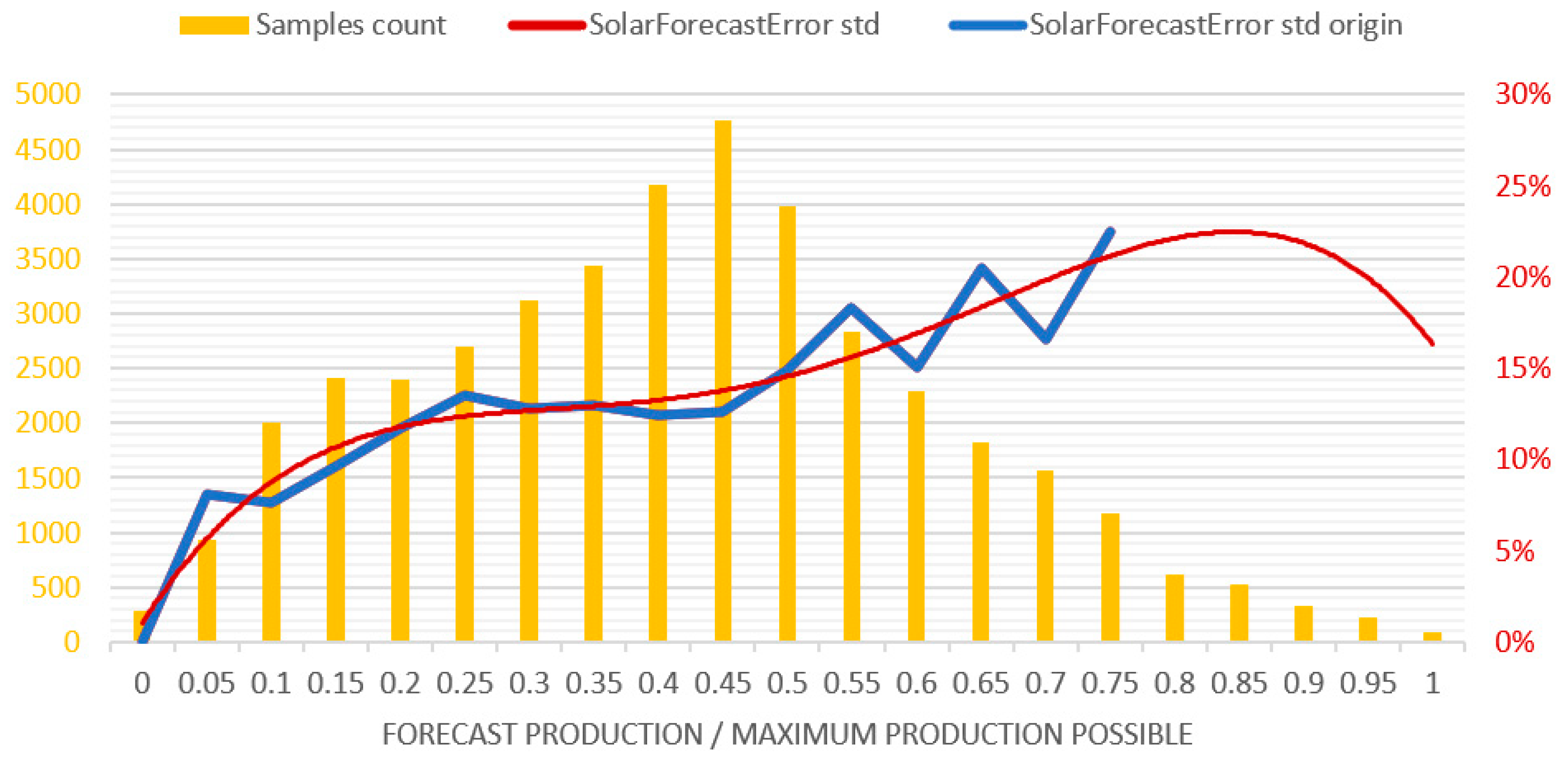
Then, solar-forecast error was grouped for every hour and zone on the basis of the ratio between forecasted PV production and maximal possible production (indirectly representing the CI through it). Thus, standard-deviation distribution was calculated as a function of this ratio.

$${\mathsf{\sigma }}_{\mathrm{solar}}^{\left(\frac{\mathrm{FP}}{\mathrm{MP}}\right)}[\%]=\mathrm{f}\left(\frac{\mathrm{ForecastProduction}}{\mathrm{MaximumProduction}}\right)$$

(23)

Figure 17 reports the obtained result for the solar-forecast-error standard deviation as a function of the above-mentioned ratio. Yellow reports the number of available samples for each category, while the exact standard deviation is shown in blue. Differently from the usual evaluation proposed by the scientific literature, the standard deviation of the PV forecast error did not decrease as the CI approximated to 1. This problem is because most PV power plants in Italy are currently not observable by the TSO since they are installed in medium- and low-voltage grids; consequently, monitoring error grows with the theoretical PV injection. Moreover, few observations are available for CI values above 0.8, affecting process accuracy (outliers impact too-high results); consequently, samples above a CI equal to 0.8 were trunked.

The contribution of solar-forecast error to nonspinning reserve was computed as

$${\mathsf{\sigma }}_{\mathrm{SOLAR}}^{\mathrm{i}\in \left(\frac{\mathrm{FP}}{\mathrm{MP}}\right)}\left[\mathrm{MW}\right]{=\mathsf{\sigma }}_{\mathrm{solar}}^{\left(\frac{\mathrm{FP}}{\mathrm{MP}}\right)}[\%]{\ast \mathrm{P}}_{\mathrm{PV},\mathrm{i}}^{\mathrm{MAX}}$$

(24)

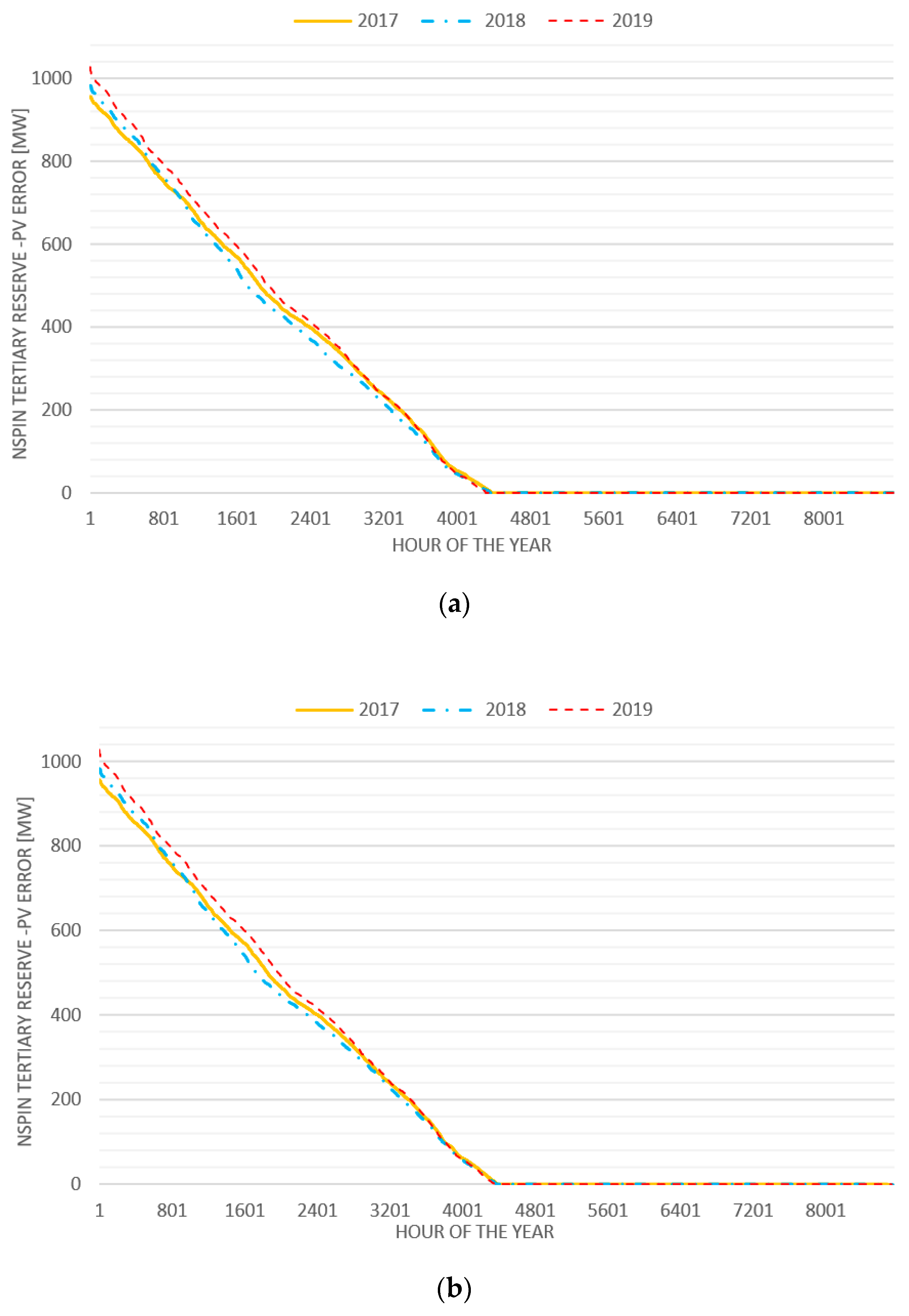
Lastly, the contribution was limited to being lower than 2/3 of the forecasted PV production for upward reserve, and lower than 2/3 of the difference between maximal production and forecasted production for the downward reserve. Figure 18a,b present the load-duration curve for upward and downward contributions to nonspinning reserve coming from solar-forecast error in the analyzed time period for the northern zone. The behavior among the different investigated years was quite similar.

4.5. Total Nonspinning-Reserve Need

Lastly, the overall need for nonspinning upward and downward reserve was calculated for the northern zone. Figure 19a,b represent the upward and downward, respectively, total nonspinning-reserve-need duration curve for the analyzed period.

5. Critical Discussion of Obtained Results

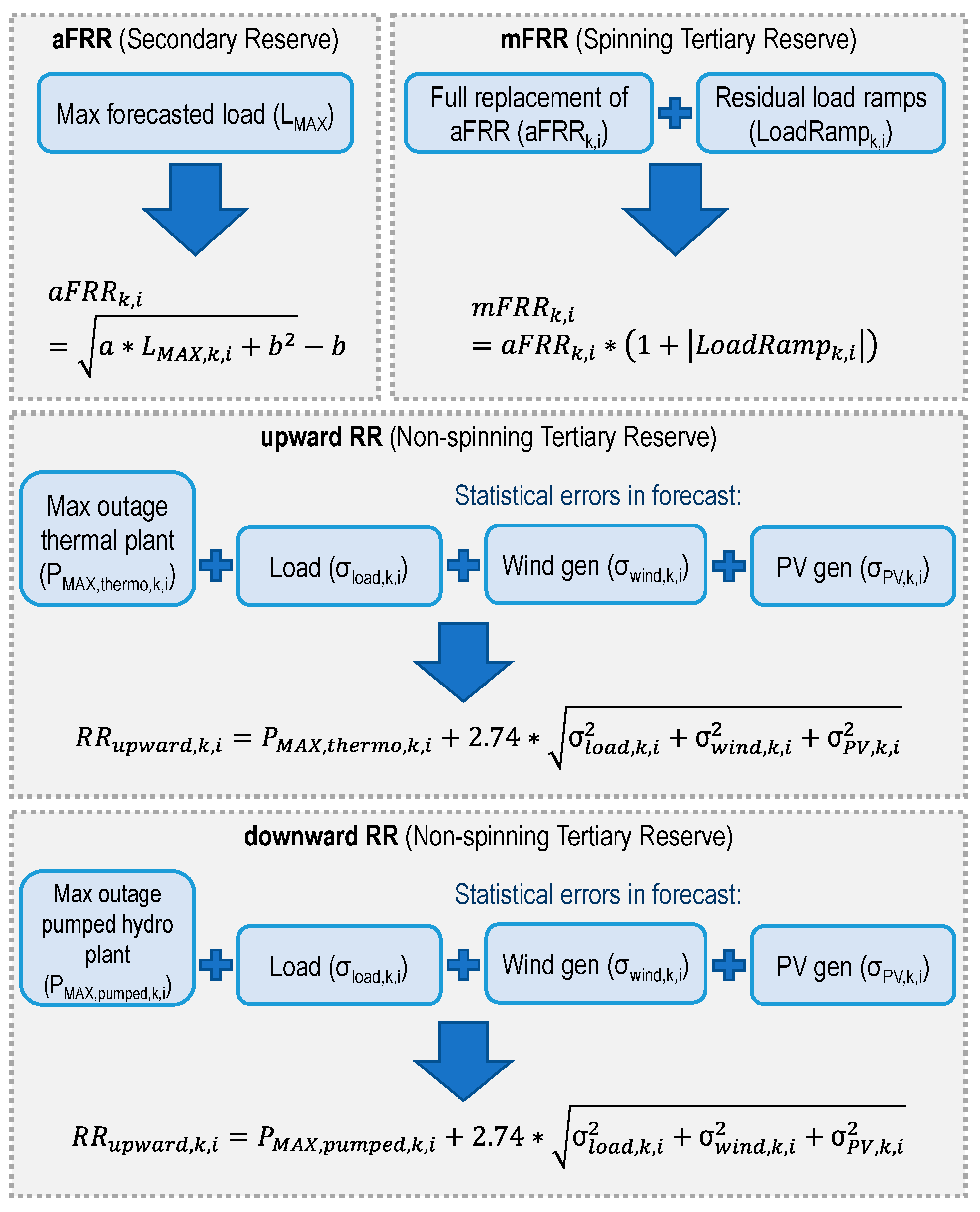
The paper established a procedure to calculate secondary- and tertiary-reserve needs over a specific control zone. The adopted approach is summarized in Figure 20, and was tested over the bidding zone of northern Italy. The first step consisted of the definition of the aFRR reserve need, which could be computed exploiting the ENTSO-e methodology, starting from the forecasted maximal load for the considered area. The calculated value for the aFRR was corrected depending on forecasted load ramp (i.e., forecasted variation of the load between subsequent hours) to determine the mFRR reserve need. Lastly, the RR reserve need was defined considering two different issues: the unexpected outage of the largest thermal (pumped hydro) power plant able to provide upward (downward) regulation, and the combination of statistical errors related to the forecast of load consumption, and wind and solar generation. All these contributions were evaluated on the basis of historical data available for 2017, 2018, and 2019. The procedure can be applied for both upward and downward regulation reserves.

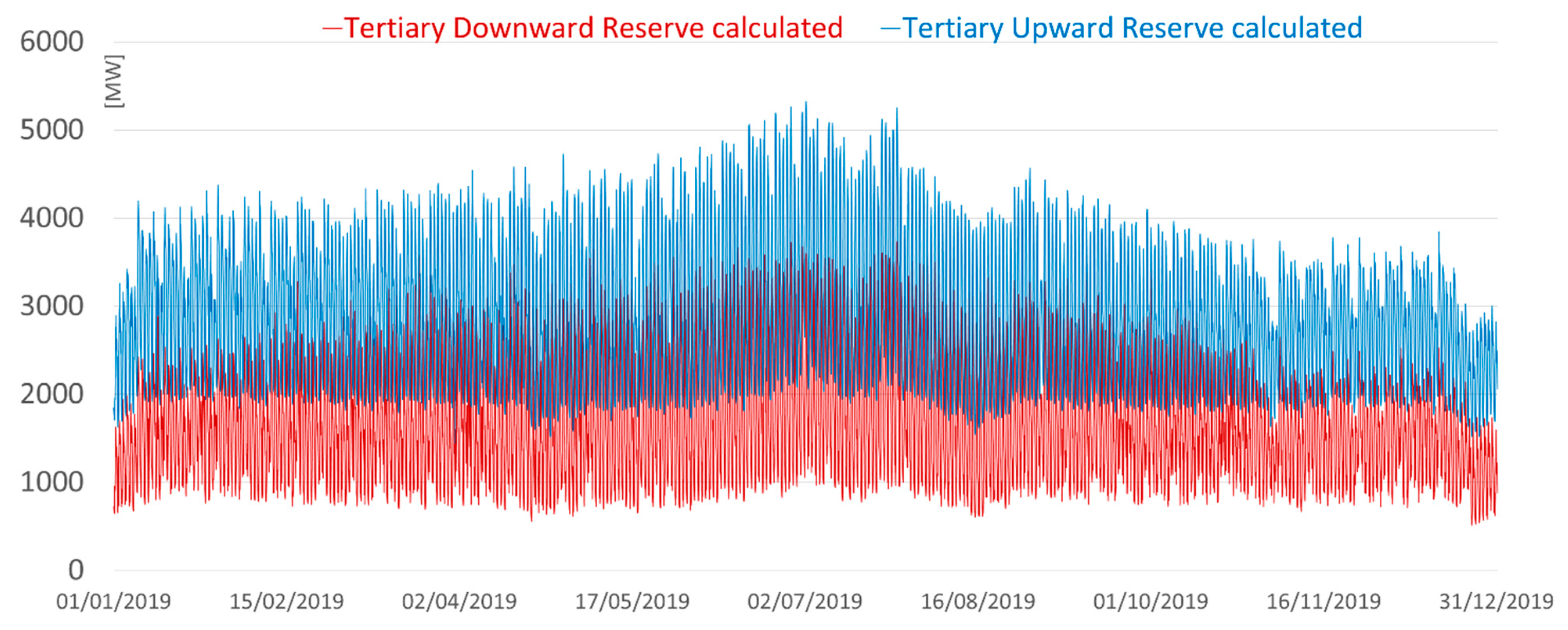
In the end, the described approach showed a positive outcome in being able to determine secondary- and tertiary-reserve needs for a specific bidding zone. This is confirmed by Figure 21, which shows the calculated values for both upward and downward tertiary reserve needs in 2019 for the bidding zone of northern Italy. The dependence of reserve need on load and solar production is also evident from the behavior reported in the figure, where the required reserve trend shows a high-frequency component with daily periodicity, and a low-frequency component mainly related to seasonality.

Unfortunately, besides past and current documents available from European and Italian TSOs mainly dealing with the available methodologies to calculate reserve needs, which were already cited, it is not possible to compare the obtained results with official data. Some of the relevant data are not public, while other available data are aggregated for a wider set of market products because, within the Italian balancing market, there is a single product exploited by Terna to provide a set of different dispatching resources. In particular, the ancillary service associated to tertiary-reserve provision can actually be used to also provide congestion resolution (only in the integrated scheduling phase), mFRR, RR, and voltage regulation.

6. Conclusions

A data-driven methodology to estimate secondary- and tertiary-reserve needs was presented, which was tested and validated over a numerical real-life case study focused on the northern Italy geographical zone. The lack of referenced EU-wide approaches to balancing reserve calculation, together with the increasing importance of balancing capacity in market scenarios with high renewables penetration, highlights the relevance of the developed procedure. The latter relates to the provision of a specific tool to evaluate and predict reserve needs to National Regulatory Authorities (NRA), market operators, and other stakeholders of the electricity sector. This can have a twofold target: on the NRA side, it can be exploited for cost–benefit analyses or to help in designing new regulatory instruments; on the operator side, it could be useful in understanding and anticipating (in a marketwise perspective) the needs of TSOs in managing grid security.