Reducing Energy Consumption and Increasing the Performances of AC Motor Drives Using Fuzzy PI Speed Controllers

Abstract

Alternating current electric drives are widely used in many commercial applications. Increasing energy efficiency and improving the quality of regulation are major goals. The speed control structure of the induction machine with indirect vector control with rotor flux orientation and the speed control structure of the permanent magnet synchronous machine with vector control with rotor flux orientation are taken into account. The control structures were modeled and simulated in Simulink. Different simulation regimes were made for different load torques and different parameters. Following the analyses performed, it was highlighted that the fuzzy regulation ensures the reduction of the energy consumption in transient states and the improvement in the quality indicators of the regulation. The fuzzy control systems are robust to the errors of identification of the machine parameters and to the effect of the disturbing load torque.

1. Introduction

Reducing energy consumption throughout the operation of an electric drive is an important goal in the design of automatic control structures for electric machines. The use of fuzzy PI regulators in the control of electric drives is a feasible solution that ensures the reduction in electricity consumption and the improvement of regulation performances. In recent years, numerous papers have appeared in the literature dealing with the use of fuzzy PI regulators in such applications.

From the specialized literature, we can mention some works such as an application on smart energy management based on a control scheme, which integrates a fuzzy logic controller within a voltage-oriented control strategy, implemented, and simulated in Simulink [1]; a systematic categorization of multi-motor techniques with a review of fuzzy logic controllers and their functionalities in multi-motor control [2]; and an application of a reversible three-phase PWM converter in a wide range of AC voltage and DC voltage drives by using a double fuzzy PI controller [3]. The development of a power supply control system based on fuzzy logic for an electric vehicle, in order to minimize the total energy consumption and optimize the battery operation, is presented in [4]. The paper shows improvements in some dynamics such as overshoot, settling time, and steady-state error parameters. It is shown that this fuzzy controller increases the overall energy efficiency of the vehicle. A type-2 fuzzy logic controller as the speed controller, acting as the driver model controller in autonomous electric vehicles, is presented in [5] as an alternative to save energy and to preserve the performances. Several other recently published papers dealing with the problems of fuzzy control of electric drives may be mentioned, as follows. A type 1 Mamdani fuzzy logic controller for electric vehicle drive is discussed in [6]. A real time adaptive speed control system of vector controlled induction motor drive based on online trained type 2 fuzzy neural network controller is presented in [7]. The role of optimization algorithms based on fuzzy controller in achieving induction motoir performance enhancement is analyzed in [8]. An experimental setup for implementation of fuzzy logic control for indirect vector-controlled induction motor drives is presented is presented in [9].

The technology of control electric drives has been developed based on new control methods such as fuzzy logic, field-oriented regulation theory, and digital equipment based on advanced microprocessors. The problem of intelligent control of electric drives has been addressed in numerous papers over the years including the application of expert systems, fuzzy logic, and neural networks in electric drives [10]; fuzzy control of switched reluctance motor drives [11]; or fuzzy adaptive vector control of induction motor drives [12]. The control structure of AC drives were developed based on the basic theory and principles from the literature as follows. The induction motors and the permanent magnet synchronous motors are the main actuators in industrial and commercial use, which offer energy savings and system optimization, and their control structures were developed using the principles presented in [13,14,15,16]. The modeling and simulation of electric drive control systems were made based on the principles presented in [17]. The development of the fuzzy PI controllers was made based on the theoretical bases of the design of fuzzy PID controllers presented in [18]. The author has researched the field of fuzzy control of electric drives and has published works in the literature, as follows. Fuzzy control systems for DC drives and permanent magnet synchronous are presented in [19] and respectively in [20]. The demonstration of the robustness of fuzzy control systems is presented in [21]. Methods of designing PI fuzzy controllers based on a pseudo-equivalence with linear controllers are presented in [22,23,24]. A method to assure the stability of fuzzy control systems based on fuzzy PI controllers is presented in [25]. Additionally, some properties of fuzzy systems useful in control systems are presented in [26,27,28].

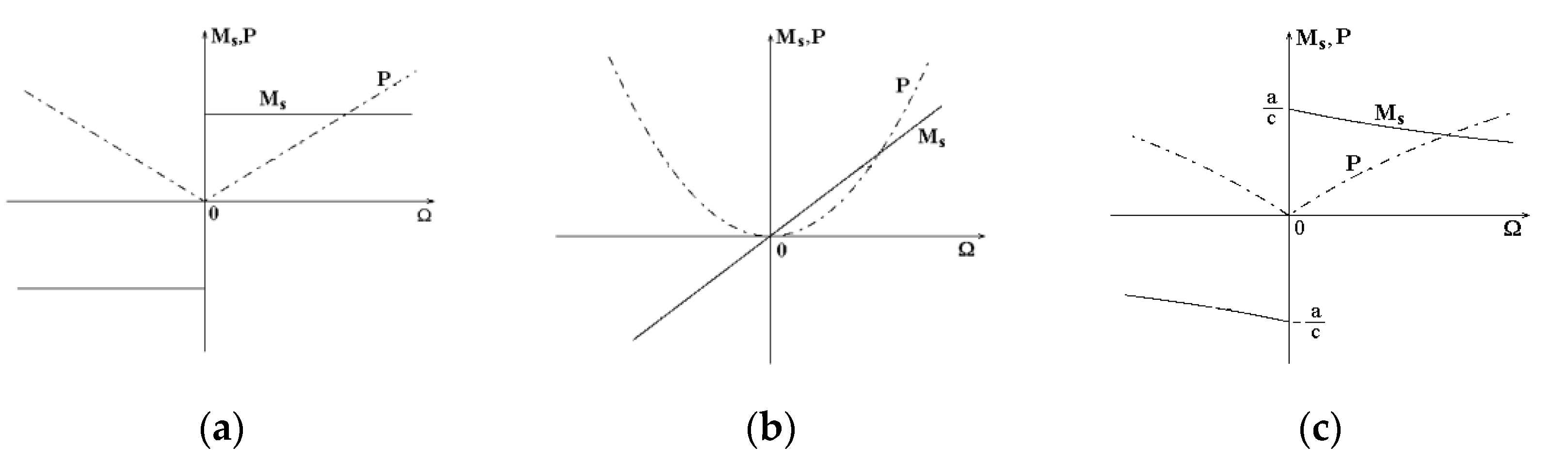
The paper presents a consideration of two digital fuzzy control structures of the two main AC machines used in practice: induction motors and permanent magnet synchronous motors. For each control system, the transient state characteristics obtained by simulation with Simulink are presented. Three types of load torques, common in practice, are considered. Transient state analyses are performed for nominal values of the machine parameters as well as in the case in which the machine parameters suffer a deviation of 100% from the nominal values. Based on the transient state characteristics, the values obtained for the performance indicators of the control systems can be highlighted such as overshoot, rise time, error, and others. A practical experiment conducted with a speed control system of a permanent magnet synchronous motor with a Hall sensor encoder, fed by a three phase inverter, based on a signal processor, demonstrated that by using fuzzy PI controllers, some performance indicators may be improved, obtaining a shorter rise time and a zero overshoot. An example of the calculation of the reduction in energy consumption is presented. The novelty of the paper is a synthetic analysis performed on the main alternating current machines by modeling and simulation, for nominal values and with deviations of the machine parameters, for three different types of load torques, resulting in 24 cases of analysis, with each case calculating the performance indicators of the regulation, demonstrating for each case that using fuzzy PI controllers obtains a reduction of the consumed energy, the improvement of the performance indicators, and the robustness of the control system.

2. Control Structures

2.1. Induction Motor

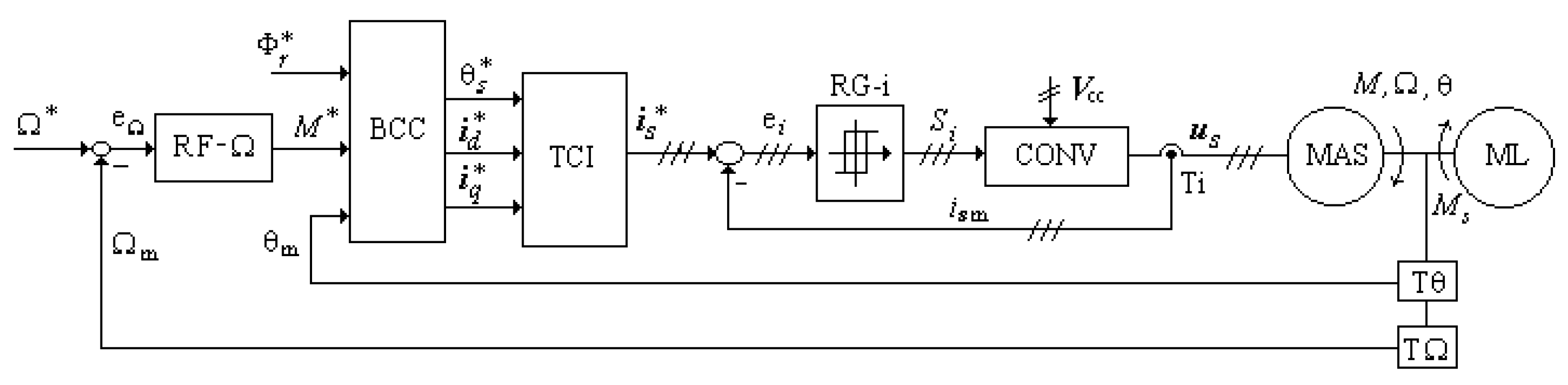
The block diagram of the fuzzy speed control structure for induction motors is presented in Figure 1.

The meanings of the notations in the Figure 1 are as follows: MAS—induction machine; ML—working machine; CONV—power electronic convertor; RG-i—stator phase current controllers; Ti—current sensor; Tθ—position sensor; TΩ—speed sensor; TCI—inverse Park coordinate transformation [14]; BCC—block for calculating the reference currents in the vector control structure of the asynchronous machine with rotor flux orientation [14,29]; RF-Ω—speed fuzzy PI controller; Ω—rotor speed; Ω*—speed reference; M*—torque reference; ф_r*—rotor flux reference; θ_s*—stator phasor position reference; i_d*, i_q*—d, q stator current references; i_s*—stator current reference; Ω_m—measured speed; θ_m—measured rotor position; i_sm—measured stator currents; e_Ω—speed error; e_i—current error; S_i—control signals for power converter switches with pulse width modulation; V_cc—DC converter supply voltage; u_s—stator voltages; M_s—load torque. The induction motor is vector controlled with rotor flux orientation, with rotor flux reference ϕ^*_r and torque reference M^* and the measured rotor position θ_m. The reference stator currents are calculated with the block TCI. The current regulators RG-i give the pulse width modulation signals S_i for the electronic power convertor CONV, fed from a DC voltage source V_CC. The power converter CONV gives the stator voltages u_s.

The mathematical model of the induction machine [14,29,30] is given by Equation (1) for a general flux orientation, where in the case or rotor orientation θ_f = θ_r.

$$\begin{gathered} {\underset{\_}{u}}_{sf}={\underset{\_}{u}}_s{e}^{-j{\mathsf{\theta }}_f},{\underset{\_}{i}}_{sf}={\underset{\_}{i}}_s{e}^{-j{\mathsf{\theta }}_f},{\underset{\_}{\Phi }}_{sf}={\underset{\_}{\Phi }}_s{e}^{-j{\mathsf{\theta }}_f},{\underset{\_}{u}}_{rf}={\underset{\_}{u}}_r{e}^{-j{\mathsf{\theta }}_f+\mathsf{\theta }},{\underset{\_}{i}}_{rf}={\underset{\_}{i}}_r{e}^{-j{\mathsf{\theta }}_f+\mathsf{\theta }}, \\ {\underset{\_}{\Phi }}_{rf}={\underset{\_}{\Phi }}_r{e}^{-j{\mathsf{\theta }}_f+\mathsf{\theta }},{\underset{\_}{u}}_{sf}=R_s{\underset{\_}{i}}_{sf}+\frac{d{\underset{\_}{\Phi }}_{sf}}{dt}+j{\omega }_f{\underset{\_}{\Phi }}_{sf},{\underset{\_}{u}}_{rf}=R_r{\underset{\_}{i}}_{rf}+\frac{d{\underset{\_}{\Phi }}_{rf}}{dt}+j({\omega }_f-\omega ){\underset{\_}{\Phi }}_{rf}, \\ M=\frac{3}{2}{n}_p{L}_m\mathrm{Re}\{j{\underset{\_}{i}}_{sf}.{\underset{\_}{i}}_{rf}^{*}\},J\frac{d\mathsf{\Omega }}{dt}=M-k_f\mathsf{\Omega }-M_s \end{gathered}$$

(1)

The other notations in Equation (1) have the following meanings: u_sf, i_sf, Ф_sf—stator voltage, current, and flux, respectively, where the notation f means with general flux orientation; u_rf, i_rf, Ф_rf—rotor voltage, current, and flux, respectively; R_s—rotor resistance; L_m—magnetic flux inductance; ω—rotor frequency; ω_f—stator frequency; J—motor inertia; k_f—friction coefficient.

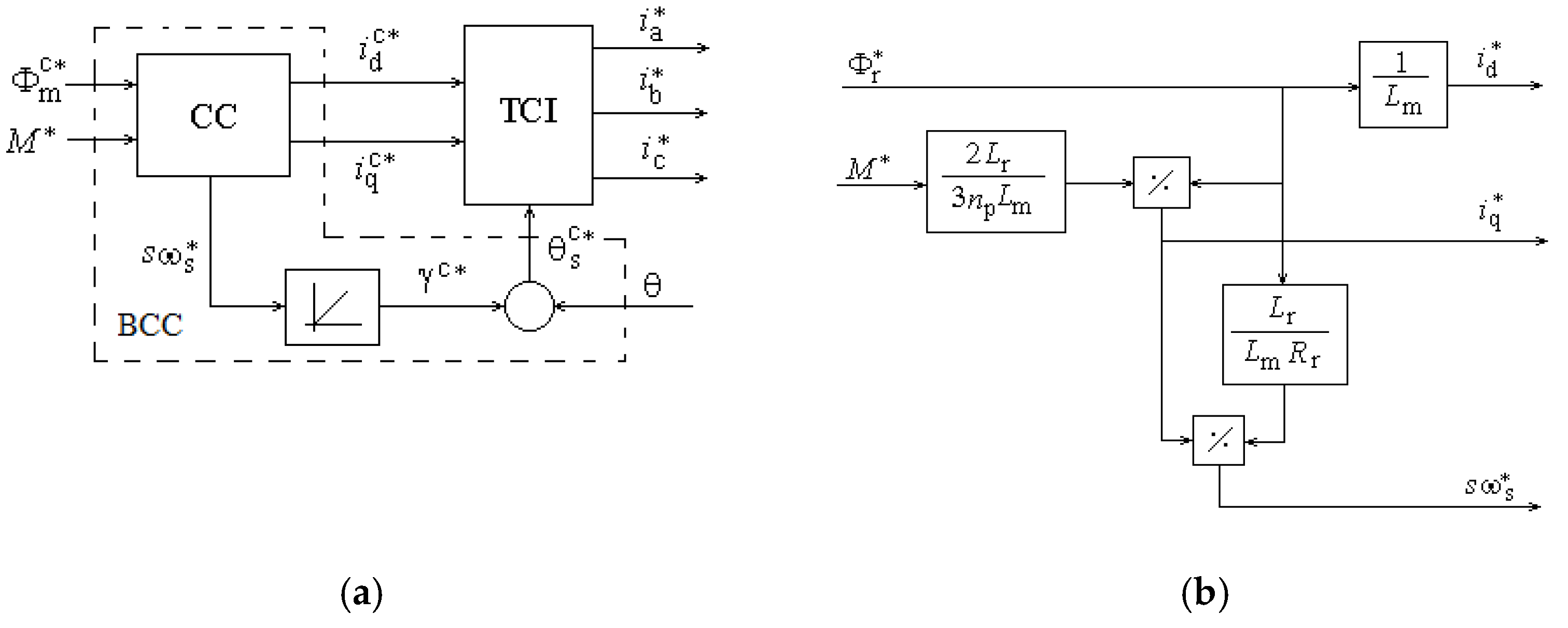
The block for calculating the reference currents in the vector control structure of the asynchronous machine with rotor flux orientation BCC has the block diagram from Figure 2a [14,29,31]. where the block CC has the structure from Figure 2b and the general magnetic flux ϕ_m^c* is the rotor flux Ф_r*; n_p—is the pole pair number; L_m,r—magnetic and rotor inductances; s—slip frequency; R_r—rotor resistance; ω_s^*—stator frequency reference.

Two-position current regulators RG-i with hysteresis were used, considering an unfavorable regulation case.

Calculation values of the induction motor were: R_s = 12.4 $\mathsf{\Omega }$; R_r = 124 $\mathsf{\Omega }$; L_m = 0.8 H; L_sσ = 0.06 H; L_rσ = 0.06 H; p = 4; k_f = 0.008 Nms; J = 0.01 kgm²; M_Mc = 7 Nm; M_Mt = 24 Nm; Ω_b = 750 rot/min; P_N(Mc) = 550 W; I_sN = 1.77 A; I_sM = 8 A; U_sN = 220 V.

2.2. Permanent Magnet Synchronous Motor

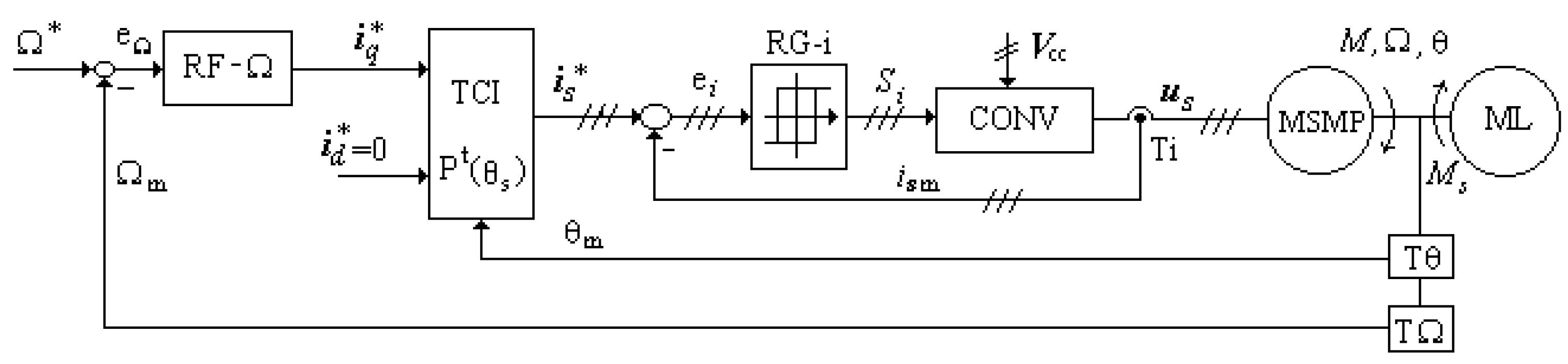
The block diagram of the fuzzy speed control structure for permanent magnet synchronous motor is presented in Figure 3 [20].

The meanings of the notations in Figure 3 are the same as in Figure 1, and MSMP is the permanent magnet synchronous machine. The permanent magnet synchronous motor is vector controlled with rotor flux orientation [15,29,30] with rotor q current i^*_q as a torque reference, the rotor d current i^*_d at zero as a flux reference ϕ^*_r, and the measured rotor position θ_m.

The mathematical model of the permanent magnet synchronous machine [15,29,30] is given by the Equation (2).

$$\begin{gathered} {\underset{\_}{u}}_{sf}={\underset{\_}{u}}_s{e}^{-j\mathsf{\theta }},{\underset{\_}{i}}_{sf}={\underset{\_}{i}}_s{e}^{-j\mathsf{\theta }},{\underset{\_}{\Phi }}_{sf}={\underset{\_}{\Phi }}_s{e}^{-j\mathsf{\theta }},{\underset{\_}{u}}_{sf}=R_s{\underset{\_}{i}}_{sf}+\frac{d{\underset{\_}{\Phi }}_{sf}}{dt}+j\omega {\underset{\_}{\Phi }}_{sf}, \\ M=\frac{3}{2}\mathrm{Re}\{j{\underset{\_}{\Phi }}_{sf}.{\underset{\_}{i}}_{sf}^{*}\},J\frac{d\mathsf{\Omega }}{dt}=M-k_f\mathsf{\Omega }-M_s \end{gathered}$$

(2)

The notations in Equation (2) are similar to those in Equation (1).

Calculation values of the permanent magnet synchronous motor were: P_N = 400 W; I_N = 3 A; I_M = 8 A; n_m = 4000 rot/min; n_b = 3000 rot/min; M_Mc = 1.3 Nm; M_Mt = 3.4 Nm; J = 0.001 kgm²; k_f = 0.0001 Nms; R_s = 0.6 Ω; L_d = 4 mH; L_q = 5 mH; p = 4; Φ_e0 = 0.072 Wb; V_cc = 200 V.

2.3. Fuzzy PI Controller

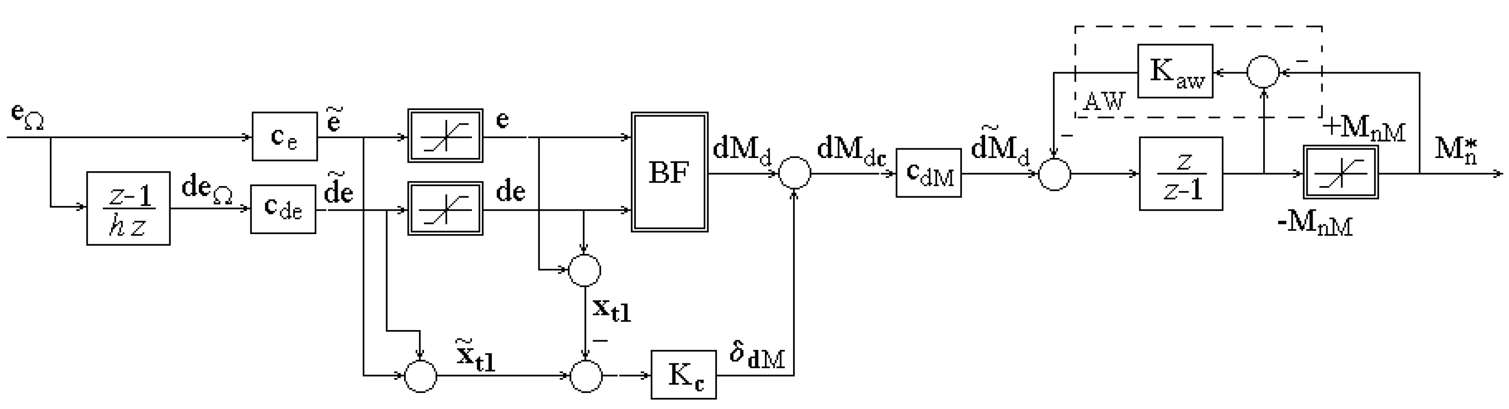
The block diagram of the fuzzy speed controller RF-Ω is presented in Figure 4.

The meanings of the notations in Figure 4 are: e—scaled angular speed error; de—scaled derivative of angular speed error; dM_d—reference of the derivative of torque M; AW—anti-wind-up circuit; M^*—torque reference; c_e, c_de, c_dM—scaling coefficients; x_t1—compound variable; BF—fuzzy block.

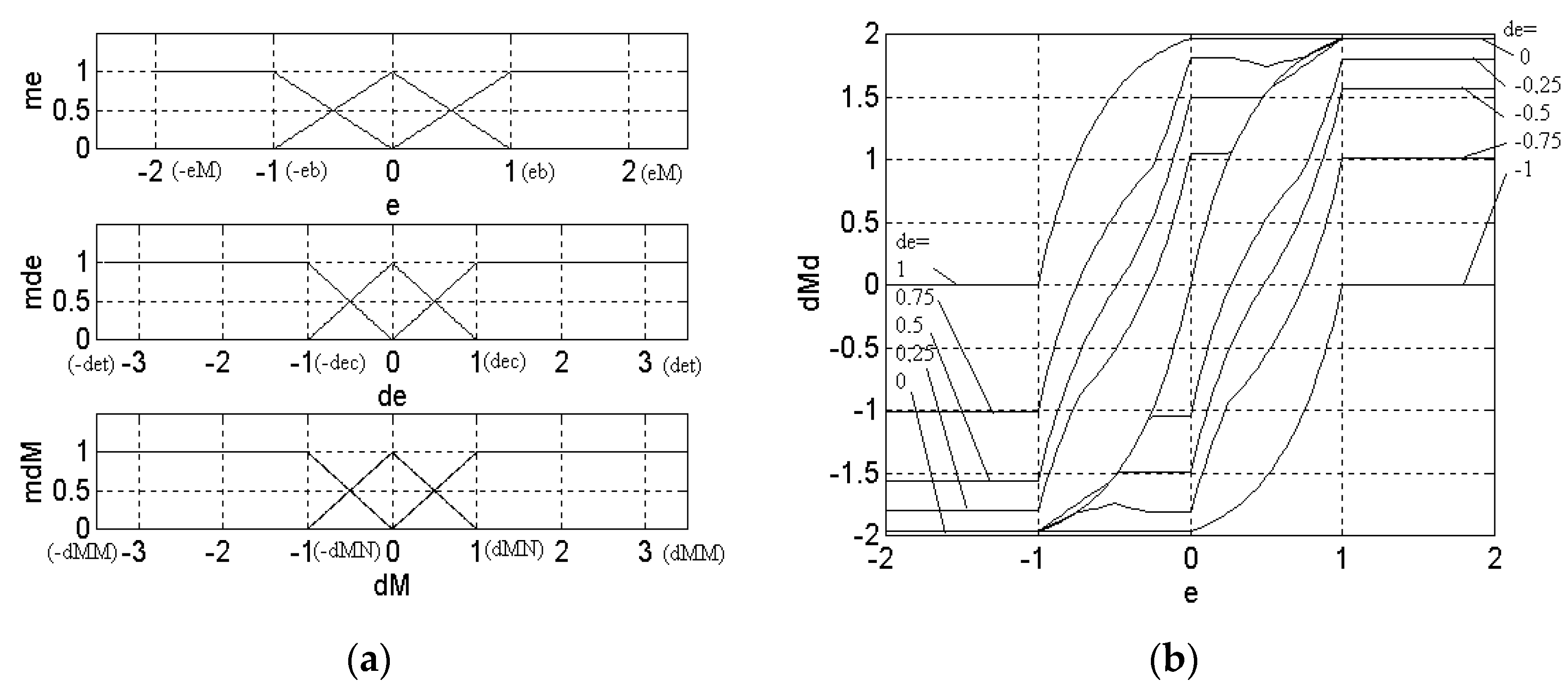
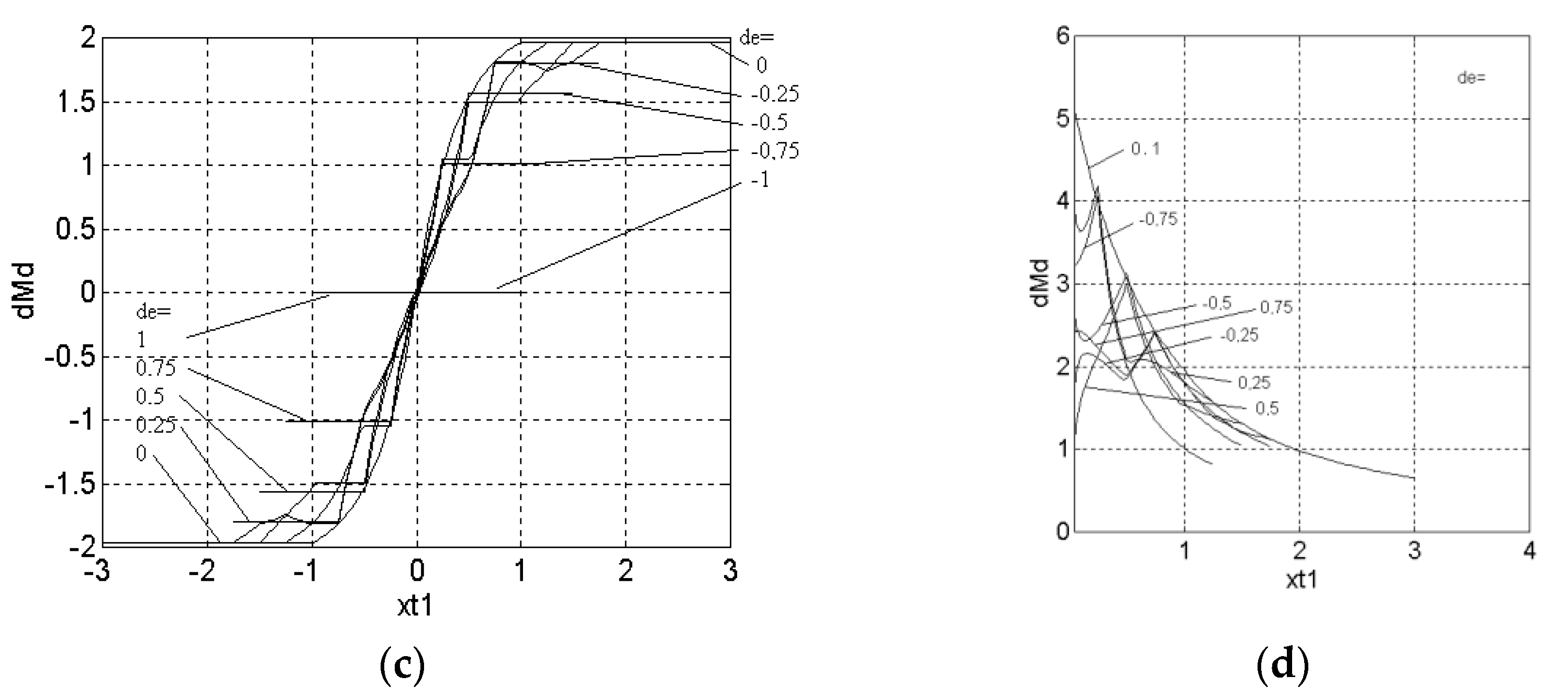
The fuzzy block BF is designed based on the principle of Mamdani, with fuzzification, rule base with nine rules, maxim-minim inference, and defuzzification with center of gravity [18,19,20]. For the input and output variables, three fuzzy values were chosen: negative, positive P, and zero Z—with the membership functions from Figure 5a. This configuration of fuzzification, inference, and defuzzification gives the highest nonlinear character for the fuzzy block [26,27,28], useful to improve control performances [19,21].

The fuzzy block BF may be analyzed based on the transfer characteristics presented in Figure 5 [19,22].

The membership functions for the two inputs and one output are presented in Figure 5a. The transfer characteristics dM_d = f_e(e; de) are presented in Figure 5b, were e is the variable and de is the parameter. The characteristics dM_d = f(x_t1; de) are presented in Figure 5c, were x_t1 is a compound variable, given by relation x_t1 = e + de. The gain characteristics dM_d = K_BF(x_t1; de) is given in Figure 5d.

Figure 5 shows the characteristics of the fuzzy block for the induction machine. Those for the permanent magnet synchronous motor were almost similar.

The design of the fuzzy speed regulator was conducted by a pseudo-equivalence with the linear PI regulator [19,22,23,24], based on the following reasoning. If the fuzzy block BF is linearized around the permanent regime operating point with e = 0, de = 0, and dM_d = 0, a relation of the form (3) is obtained:

$$d{M}_d=K_0(e+de)$$

(3)

The value K₀ can be determined with sufficient approximation at the limit on the characteristic families of the fuzzy blocks K_BF = (x_t1; de), see relation (4).

$$K_0=\underset{x_{t1}\to 0}{\lim }{K}_{BF}(x_{t1};0)$$

(4)

Taking into account the correction made on the fuzzy block with the torque increment coefficient c_dM, the characteristic of the corrected and linearized fuzzy block around the origin is given by the relations:

$$d{\tilde{M}}_d=c_{di}{K}_0(e+de),{\tilde{c}}_{di}=c_{di}{K}_0$$

(5)

For the fuzzy speed controller RF-Ω with the linearized fuzzy block BF, the following input–output relationship can be written in the z domain:

$$M_n^{*}(z)=\frac{z}{z-1}{\tilde{c}}_{di}[e(z)+de(z)]=\frac{z}{z-1}{\tilde{c}}_{di}\left[c_e+c_{de}\frac{z-1}{hz}\right]e_{\mathsf{\Omega }}(z)$$

(6)

With these observations, the transfer function of the fuzzy linearized RF-Ω speed controller becomes:

$$H_{RF}(z)=\frac{M_n^{*}(z)}{e_{\mathsf{\Omega }}(z)}=\frac{z}{z-1}{\tilde{c}}_{di}\left(c_e+c_{de}\frac{z-1}{hz}\right)$$

(7)

A pseudo-equivalence of the fuzzy speed controller RF-Ω can be made with a continuous speed controller such as the one chosen for conventional speed control systems:

$$H_{R\mathsf{\Omega }}\left(s\right)=K_{R\mathsf{\Omega }}\left(1+\frac{1}{s{T}_{R\mathsf{\Omega }}}\right)$$

(8)

For this, the following quasi-continuous form is used:

$$H_{RF}(s)=\frac{M_n^{*}(s)}{e_{\Omega }(s)}={H_{RF}(z)|}_{z=\frac{1+sh/2}{1-sh/2}}=\frac{{\tilde{c}}_{di}}{h}\left(c_{de}+\frac{h}{2}{c}_e\right)\left[1+\frac{c_e}{(c_{de}+c_{e}h/2)s}\right]$$

(9)

It is observed that the above transfer function resembles the transfer function (9) of the linear speed PI controller, used in the conventional control structure. The identification of the coefficients of the transfer functions (9) and (10) shows some equalities, and from these equalities are deduced the relations of expression of the scaling coefficients based on the parameters of the already existing speed regulator:

$$c_e=\frac{h{K}_{R\mathsf{\Omega }}}{c_{dM}{K}_0{T}_{R\mathsf{\Omega }}},c_{de}=c_e(T_{R\mathsf{\Omega }}-h/2)$$

(10)

where h is the sampling period.

The coefficient Kc is used to assure stability, according to the demonstration from [25]. A nonlinear correction is made to move the characteristics dM_d = f(x_t1; de), from Figure 5c, from the non-intervention area from the x axis, were dM_d has zero values for e and de different from zero, in stability sector.

2.4. Look-Up Table Implementation of the Fuzzy Block

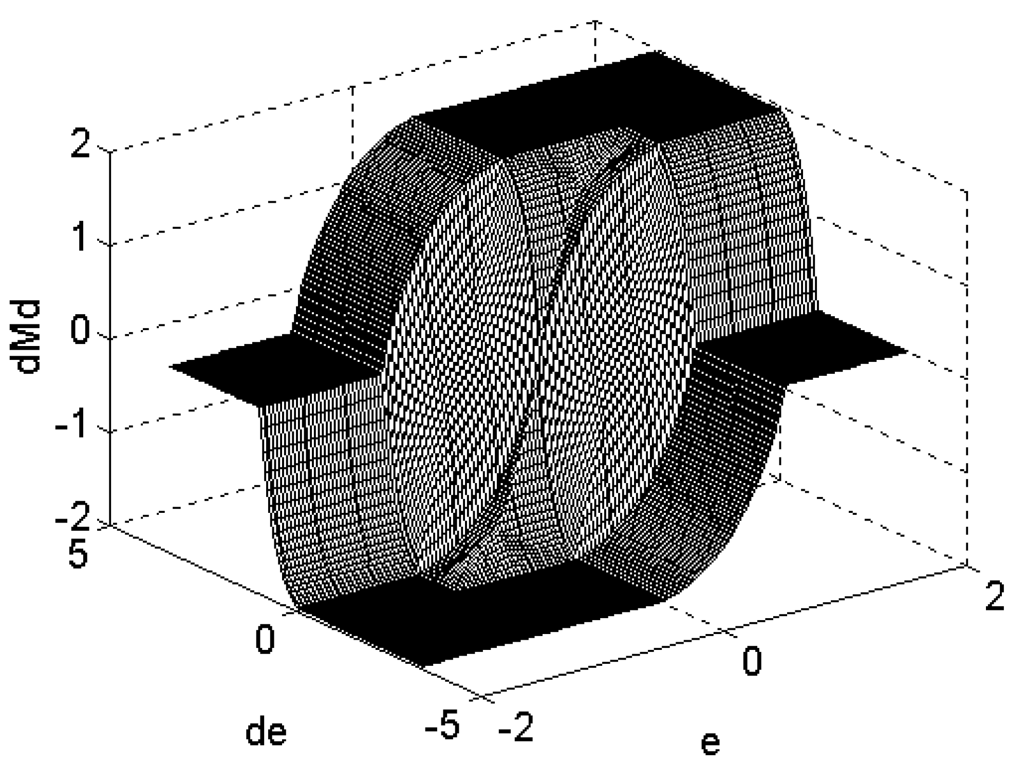
The solution for implementing the fuzzy blocks that gives the highest response speed, both in simulation and in practical applications, is the tabular implementation of the fuzzy block, in the form of a matrix, stored in the memory of the numerical control equipment. The models of the AC machine speed control structures are relatively complex, which makes the duration of a calculation step relatively long. The use of a pulse width modulation in the calculations resulted in a large number of iterations. The introduction of the fuzzy block in the simulation scheme in the form of the structure that requires the performance of fuzzification, inference, and defuzzification operations at each integration step, makes the calculation time increase even more. It is recalled that the inference method and the defuzzification method used are time consuming. The same fuzzy block computation problems arise when the practical implementation of fuzzy control on a physical control system of AC machines is required, at which an adequate real-time response speed must be ensured. The fuzzy block BF is represented by a nonlinear function of two variables dM_d = f_BF(e, de). This function is implemented tabularly, in the form of a matrix DM_d of elements dM_d(a_e, a_de), stored in the computer’s memory. Such a ‘fuzzy memory’ has a data output dM_d and two address inputs a_e and a_de. At the output, the memory shows the real value dM_d stored at the address (a_e, a_de.). Addresses have integer values. In order to create the matrix, the discourse universes of the input quantities of the fuzzy block e and de are discretized in n_c parts. By tabulating the function dM_d = f_BF(e, de) for all combinations of input values, we obtain (n_c + 1)² values for the output dM_dk = f_R(e_ae, de_ade), where a_e = 1, ..., n_c + 1 and a_de = 1, ..., n_c + 1. These values are stored in the matrix DM_d = [di_d(a_e, a_de)]. This array memory must be addressed with values a_e and a_de. For the quantity e, a translation is made from [-e_M, e_M] to [1, n_c + 1], and for the quantity de, a translation is made from [-de_M, de_M] to [1, n_c + 1]. Memory addresses are integers, so to determine them, the integer part of e_t and de_t must be calculated:

$$\begin{gathered} e_t=\frac{n_c}{2e_M}e+\frac{n_c+2}{2},d{e}_t=\frac{n_c}{2d{e}_M}de+\frac{n_c+2}{2}, \\ {a}_e=[e_t],a_{de}=[d{e}_t] \end{gathered}$$

(11)

The function of the fuzzy block BF is implemented with an approximation of it:

$$d{M}_d=f_{BF}(e,de)\cong d{M}_d(a_e,a_{de})=f_{BF}^{*}([e_t],[d{e}_t])$$

(12)

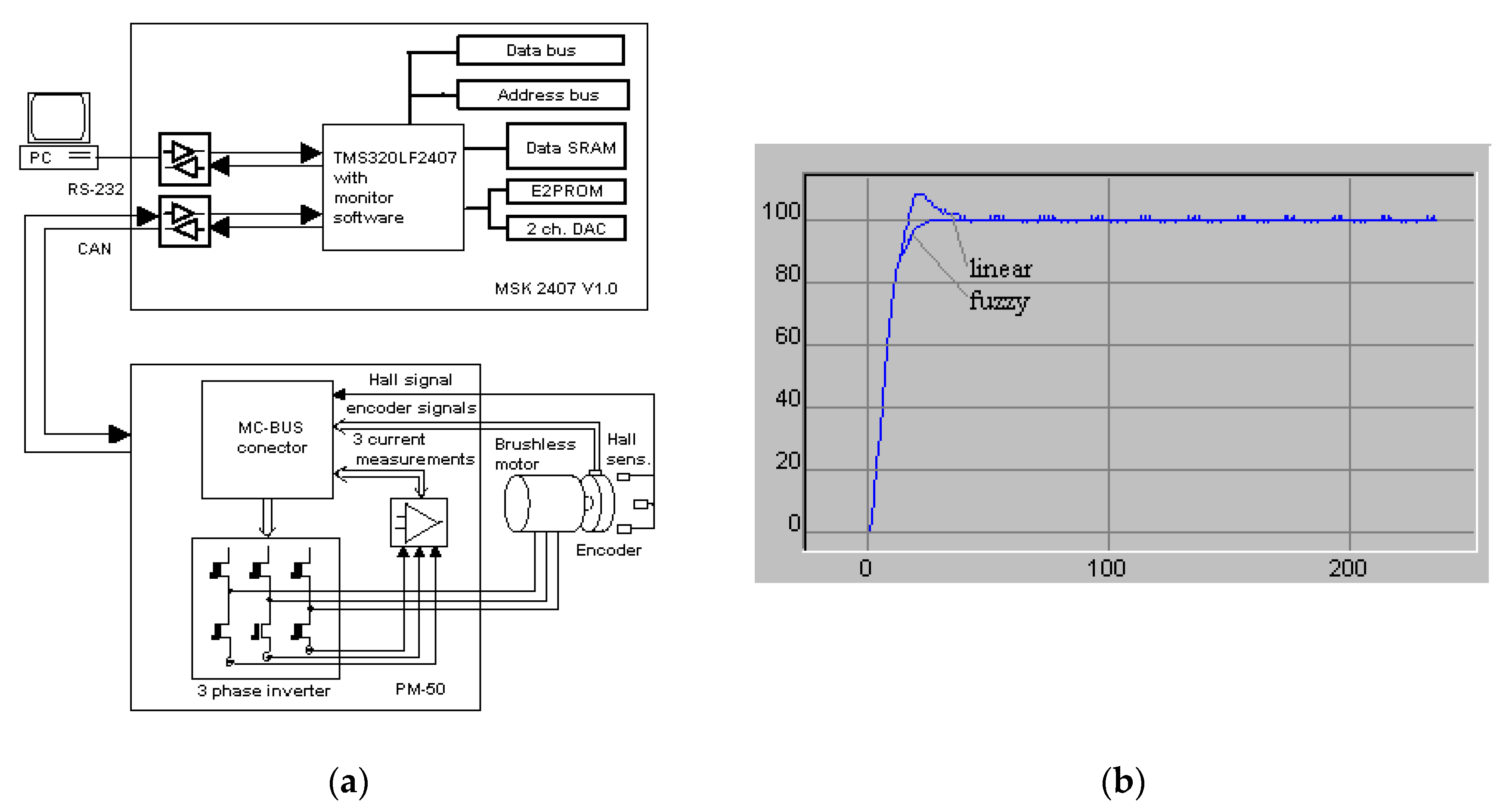
In the simulation, an implementation of fuzzy memory was chosen for an analog-to-digital converter of only eight bits, a situation that is the most unfavorable case. Figure 6 shows the multi-input-single-output (MISO) transfer surface of the fuzzy block for the asynchronous machine. It was obtained by tabulating the function f_BF(e, de) with a resolution of 1/2⁸ of the universes of discourse of the inputs.

The required memory decreases significantly. The number of samples for each speech universe becomes 2⁸ + 1 = 257. The number of memory locations required is 66.049. The required memory capacity is almost 265 KB. Such fuzzy memory can be stored in RAM during calculations. The simulations showed that even in this unfavorable case, good values of the quality indicators of the regulation can be obtained.

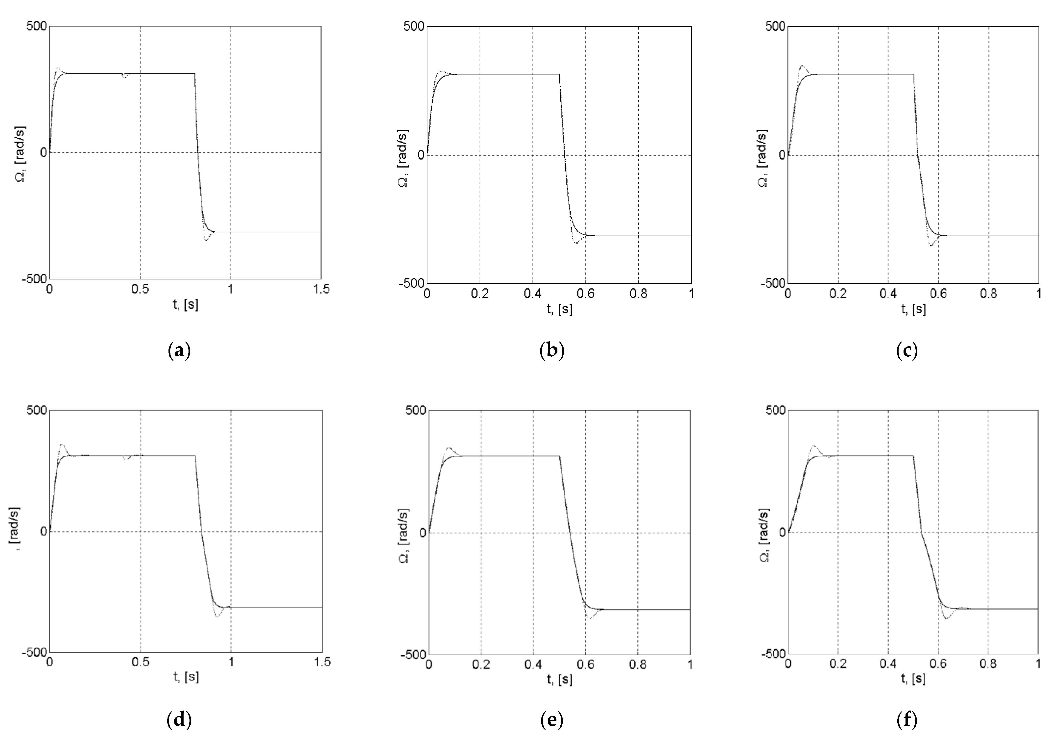
3. Results

3.1. Transient Features

3.1.1. Simulation Conditions

The analysis of the behavior of the regulation systems was done in some cases, as specified below. The abbreviated specification of the analysis cases was made according to the symbols in Figure 7.

It was chosen to analyze the behavior to the modification of the parameters in time, due to the temperature, the magnetic saturation, or the modification of the load and the case of deviations when estimating the machine parameters. The values of the parameters taken in the analysis for the case of induction machine (mas) are presented in

Table 1. The values of the parameters taken in the analysis for the induction machine (mas).

Rr [Ω]		J [kgm2]		kf [Nms]
a	d	a	d	a	d
12.4	24.8	0.01	0.02	0.0008	0.0016

and for the case of the permanent magnet synchronous machine (msmp) in

Table 2. The values of the parameters taken in the analysis for the permanent magnet synchronous machine (msmp).

Rr [Ω]		J [kgm2]		kf [Nms]
a	d	a	d	a	d
0.6	1.2	0.001	0.002	0.0001	0.0002

for the tuned case (a) and for the detuned case (d).

The results obtained using the fuzzy PI speed controller, denoted with (f), were compared with the results obtained in the conventional control case, denoted with (c) when using a linear PI speed control. The linear regulator was designed using the symmetry criterion in Kessler’s version [32], which is a currently recommended method in practice. In the case of conventional control, a smoothing element located at the prescription input of the control system is also used, which is commonly in practice [29,32].

Three types (1, 2, 3) of load torques M_s were considered [29]. Their mechanical characteristics are represented in Figure 8a–c, respectively.

In the simulation scenario with load torque 1, it was considered to start the drive unloaded, then load it with a nominal torque and then reverse it. In the simulation scenarios with load torques 2 and 3, it was considered to start the drive in nominal load and then to reverse it.

3.1.2. Induction Motor Characteristics

The transient state characteristics of the torque M and angular velocity Ω, in cases mas-1(2,3)-f-a(d), are presented in Figure 9.

For detuned parameters, the torque is greater in the transient region and the rise time is longer. The overshoot at the start and at reverse is zero. In the transient state, the machine is driven with the maximum torque. Therefore, the acceleration is maximum and the speed variation has a maximum slope.

The transient state characteristics of the angular velocity Ω, in cases mas-1(2,3)-f(c)-a(d) are presented in Figure 10.

The values of the performance criteria indicators are presented in

Table 3. Performance indicator values for the induction machine.

Analysis Case	σ1 [%]	trΩ [s]	σ1M [%]	tcM [s]	σ1r [%]	trr [s]	E .10−5	Δσ1 [%]	Δσ1M [%]	ΔtrΩ [s]	ΔtcM [s]
Mas-1-c-a	4.5	0.19	5.7	0.15	2.0	0.13	720	4.5	3.1	0.1	0.14
Mas-1-f-a	0	0.09	2.6	0.01	0	0.12	679
Mas-1-c-d	9.6	0.34	8.3	0.25	3.2	0.45	1068	9.6	6.4	0.25	0.23
Mas-1-f-d	0	0.09	1.9	0.02	0	0.15	909
Mas-2-c-a	0.6	0.09	-	-	0.6	0.16	701	0.6	-	0.01	-
Mas-2-f-a	0	0.1	-	-	0	0.12	703
Mas-2-c-d	4.4	0.12	-	-	3.2	0.23	954	4.0	-	0	-
Mas-2-f-d	0.4	0.12	-	-	0	0.13	937
Mas-3-c-a	1.9	0.19	-	-	3.8	0.22	863	1.9	-	0.08	-
Mas-3-f-a	0	0.11	-	-	0	0.14	896
Mas-3-c-d	4.5	0.32	-	-	5.1	0.33	1021	3.5	-	0.2	-
Mas-3-f-d	1.0	0.12	-	-	1.3	0.16	1011

and they are discussed in Section 4.

3.1.3. Permanent Magnet Synchronous Motor Characteristics

The transient state characteristics of torque M and angular velocity Ω, in cases msmp-1(2,3)-f-a(d), are presented in Figure 11.

The transient state characteristics of the angular velocity Ω, in cases msmp-1(2,3)-f(c)-a(d), are presented in Figure 12.

The values of the performance criteria indicators are presented in

Table 4. Performance indicator values for the synchronous machine.

Analysis Case	σ1 [%]	trΩ [s]	σ1M [%]	tcM [s]	σ1r [%]	trr [s]	E .10−5	Δσ1 [%]	Δσ1M [%]	ΔtrΩ [s]	ΔtcM [s]
Msmp-1-c-a	6.7	0.07	6.4	0.04	11.4	0.09	6.81	6.7	5.1	0.01	0.04
Msmp-1-f-a	0	0.06	1.3	0	0	0.08	6.17
Msmp-1-c-d	16.2	0.13	5.4	0.04	13.1	0.16	12.65	16.2	4.8	0.05	0.04
Msmp-1-f-d	0	0.08	0.6	0	0	0.13	11.96
Msmp-2-c-d	4.5	0.07	-	-	9.9	0.09	7.02	4.5	-	0	-
Msmp-2-f-d	0	0.07	-	-	0	0.08	6.37
Msmp-2-c-a	10.8	0.12	-	-	11.8	0.15	13.05	10.8	-	0.04	-
Msmp-2-f-d	0	0.08	-	-	0	0.12	12.29
Msmp-3-c-a	10.8	0.08	-	-	13.1	0.1	7.76	10.8	-	0	-
Msmp-3-f-d	0	0.08	-	-	0	0.1	6.99
Msmp-3-c-a	13.1	0.16	-	-	13.1	0.17	14.50	13.1	-	0.03	-
Msmp-3-f-d	0	0.13	-	-	0	0.13	13.63

and they are discussed in Section 4.

3.2. Performance Indicators

The values of the performance indicators for the induction machine control system are presented in Table 3, and the values for the synchronous machine control system are presented in Table 4. They are obtained from the above characteristics.

The meanings of the notations in the tables are: σ₁—speed overshoot at start-up; t_rΩ—rising time; σ_1M—the maximum deviation of the speed from the effect of the disturbing load torque; t_cM—time to eliminate the effect of disturbance; σ_1r—speed overshoot at reversal; t_rr—reversal rise time; E—integral criterion; Δσ₁—overshoot difference between overshoot at nominal parameters and overshoot at detuned parameters; Δσ_1M—maximum deviation difference; Δt_rΩ—rise time difference; Δt_cM—difference of torque effect elimination time. The error integral criterion has relation (13). It is integral to the square of the speed error.

$$\mathrm{E}={\displaystyle \int }{\left({\mathsf{\Omega }}^{*}-\mathsf{\Omega }\right)}^2\mathrm{dt}$$

(13)

3.3. Some Results from a Digital Implementation

In [20], the author presented an example of the implementation of a speed control system of a brushless motor with a Hall sensor encoder, based on a TMS320LF2407 DSP platform. The structure of the equipment is presented in Figure 13a.

The test platform is using a Texas Instruments motion control kit MSK 2407, monitor software, and development software installed on a personal computer (PC), a power electronic converter PM-50 with a three phase inverter and auxiliary circuits, with structures from Figure 13a. The implementation of the fuzzy block BF may be done using a look-up table, as presented in Section 2.4. This is the way that assures the minimum time response in the practical implementation of a fuzzy block. Using the fuzzy PI controller, the characteristics in Figure 13b may be obtained. This was compared with the characteristic for a linear PI speed controller. This example demonstrates that using fuzzy PI controllers may improve some performance indicators, obtaining a shorter rise time and a zero overshoot.

3.4. Example of Calculating the Reduction of Energy Consumed

Using the results obtained by simulation, from the transient state characteristics of torque and speed and the values of the performance indicators in the tables, a simple calculation of the energy difference ΔW between the energy consumed in linear regulation and the energy consumed in fuzzy regulation in transient states can be made. An empiric formula may be used:

$$∆W\cong \left(M_c{\Omega }_{\mathrm{c}}{\mathrm{t}}_{\mathrm{rc}}-M_f{\Omega }_{\mathrm{f}}{\mathrm{t}}_{\mathrm{rf}}\right)\cong \left(1.05.M_n.1.05.{\Omega }_{\mathrm{n}}{\mathrm{t}}_{\mathrm{r}}-M_n{\Omega }_{\mathrm{n}}{\mathrm{t}}_{\mathrm{r}}\right)\cong 0.1.{\mathrm{P}}_{\mathrm{n}}{\mathrm{t}}_{\mathrm{r}},$$

(14)

were M is the torque; Ω is the speed; and t is the duration of transient regime for the linear, or conventional case denoted with c and for fuzzy case denoted with f. The case of nominal speed control, denoted with n, was chosen. The duration of the longer transitional regime was chosen from the conventional case t_r. Based on the characteristics and table values, for the case of conventional regulation, it is approximated that the torque and the rotation speed were 5% higher than in the case of fuzzy regulation. Thus, it can be said that the energy difference was about 0.1 of the nominal energy consumed during the transient state.

4. Discussion

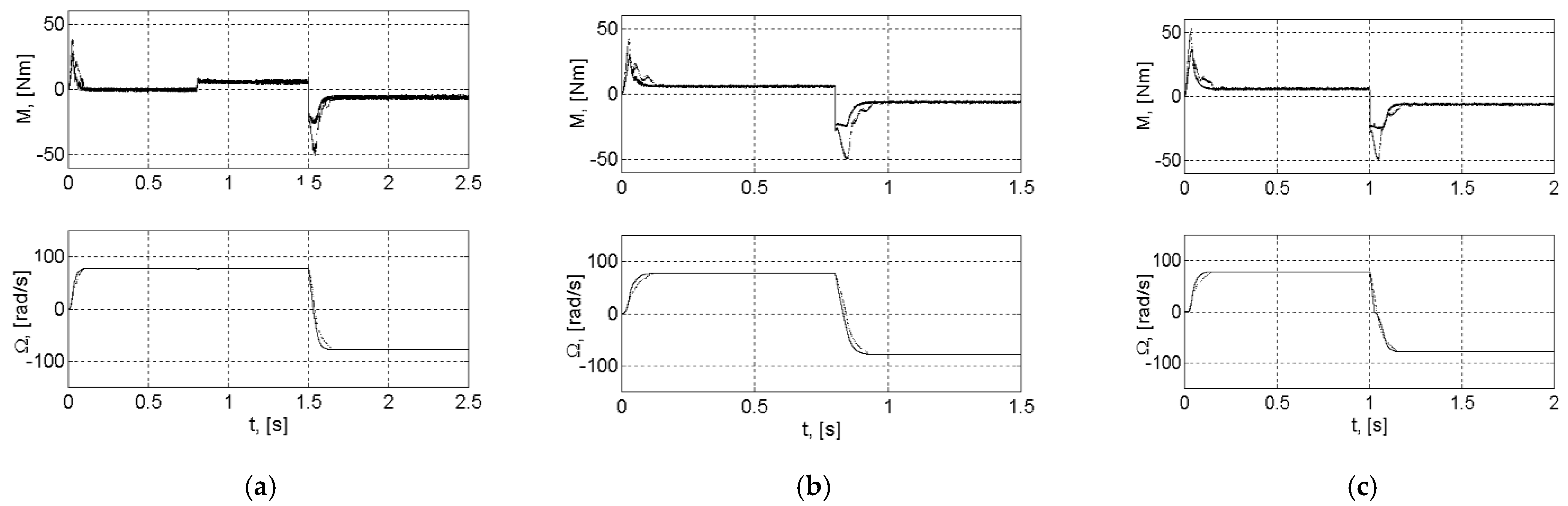
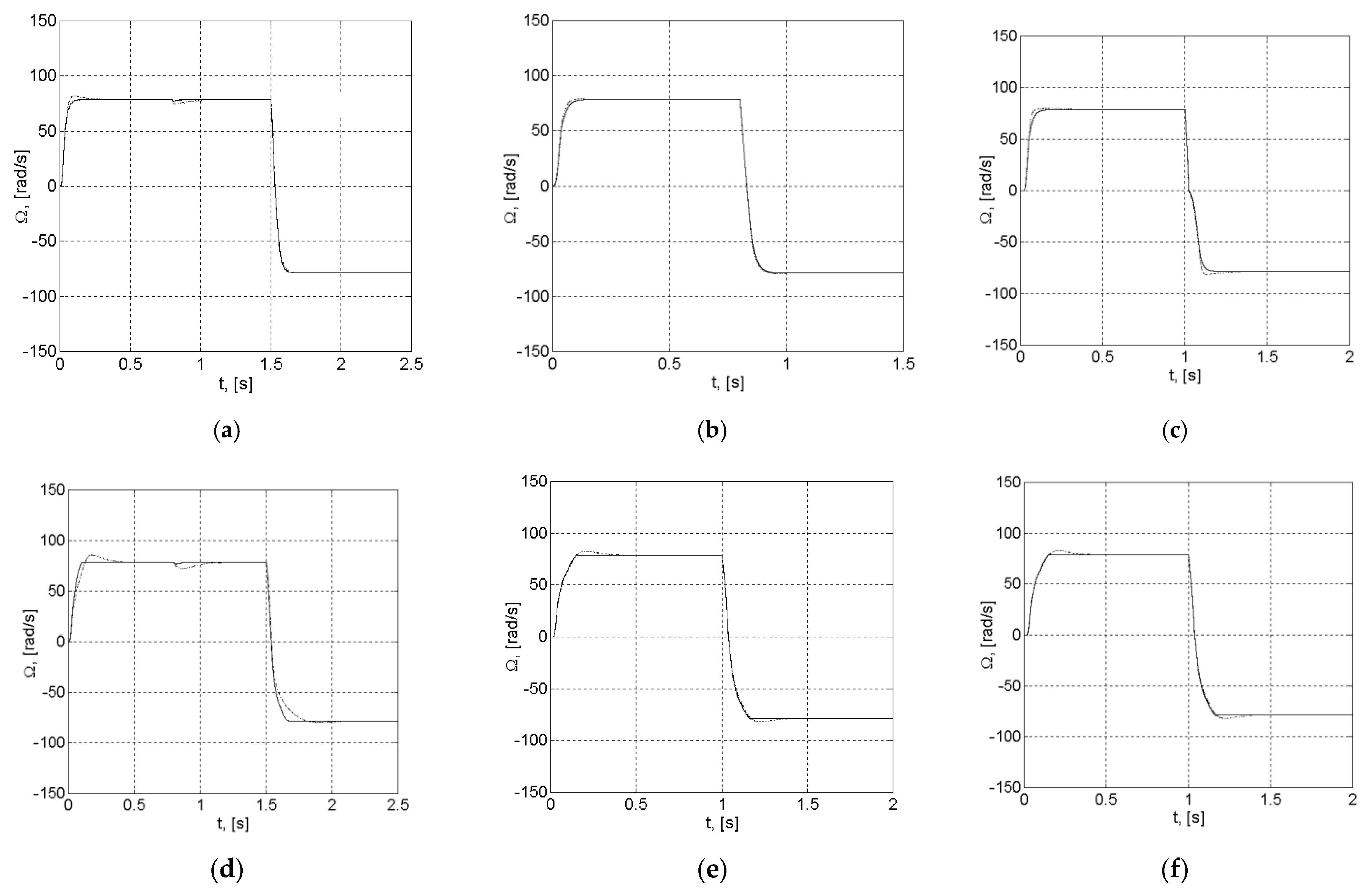
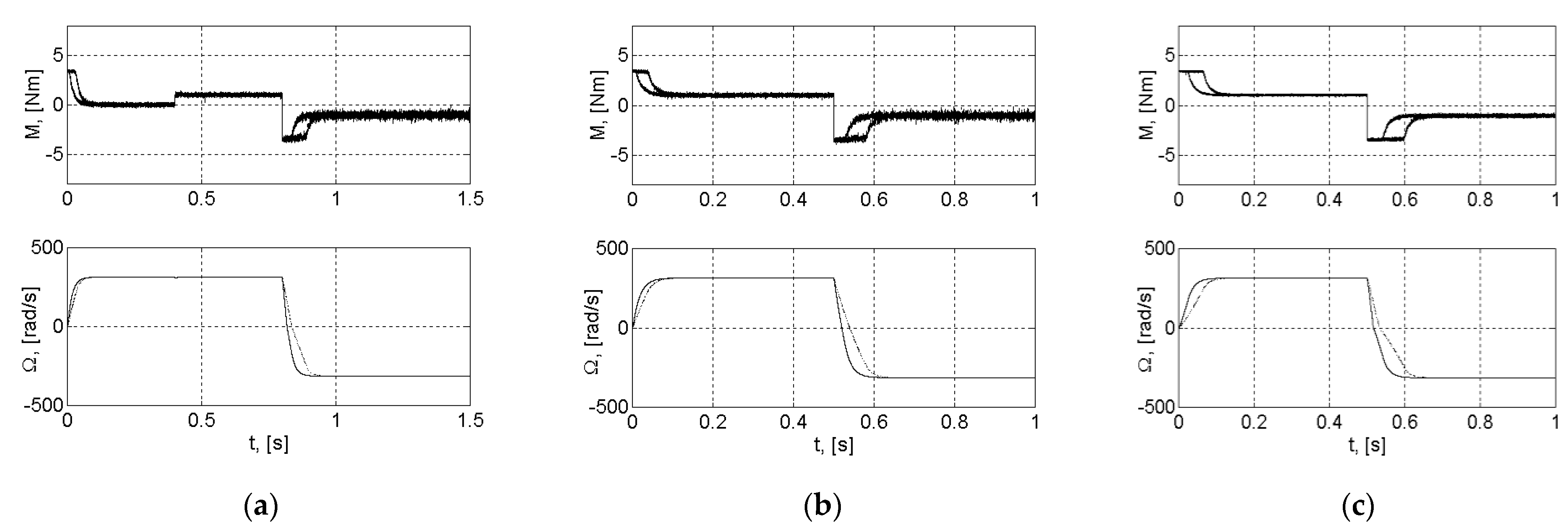
From the characteristics of the transient regime and from the values from the tables presented above, the following can be observed. Fuzzy logic-based control provides zero overshoot σ₁, unlike conventional control, which provides a greater overshoot, both in the case of tuned parameters and in the case of detuned parameters, for all three load torques. The rise time t_rΩ was smaller in all cases with fuzzy control. The effect of disturbing load torque was eliminated faster in the case of fuzzy control: t_cM and σ_1M were smaller. The reversal time t_rr was shorter for fuzzy control. The error integral criterium had smaller values for fuzzy control. The values of all quality indicators were better in the case of fuzzy control, in all cases analyzed. It should be noted that better values were obtained in the most unfavorable cases using bipositional current regulators and the implementation of fuzzy memory with the lowest resolution. The values of the torque developed by the machine in transient mode were lower in the case of fuzzy control than in the case of conventional control. The duration of the transitional regime was shorter. These aspects were valid in all cases analyzed, for different values of the parameters and for different load torques. The fact that at fuzzy control, the torque developed by the machine was lower, the speed overshoot was zero, and the duration of the transient state was shorter, leading to the conclusion that the consumed energy was smaller, which leads to energy saving.

5. Conclusions

The paper presents an analysis performed by the modeling and simulation of the behavior of the speed control structures with a fuzzy PI controller of the asynchronous machine vector controlled with indirect orientation after the rotor flux and the speed control structure with a fuzzy PI controller of the permanent magnet synchronous machine vector controlled with orientation after the rotor flux. The analyses were performed for nominal values of the machine parameters and for deviated values of the parameters by 100%. Additionally, three different types of load torques commonly encountered in practice were considered. The paper shows the design of the fuzzy regulators used. The fuzzy blocks were implemented in the tabular manner, as matrix stored in memory, the solution that gives the highest response speed.

The values obtained for fuzzy regulation were compared with the values obtained for conventional regulation with linear PI speed regulators. Linear PI regulators are the most common and widely used in commercial electric drives.

This paper demonstrates that the use of fuzzy PI regulators for regulating the speed of AC electric motors leads to a reduction in energy consumed in transient states and an improvement in the quality indicators of regulation. The paper also demonstrates that control systems based on fuzzy logic are more robust to errors in identifying the parameters of electric machines. They are also more robust to the effect of disturbing load torque.

References

1. De Luca, F.; Calderaro, V.; Galdi, V. A Fuzzy Logic-Based Control Algorithm for the Recharge/V2G of a Nine-Phase Integrated On-Board Battery Charger. Electronics 2020, 9, 946. [Google Scholar] [CrossRef]
2. Štil, V.J.; Varga, T.; Benšić, T.; Barukčić, M. A Survey of Fuzzy Algorithms Used in Multi-Motor Systems Control. Electronics 2020, 9, 1788. [Google Scholar] [CrossRef]
3. Zhang, W.; Fang, Y.; Ye, R.; Wang, Z. Analysis and Design of a Double Fuzzy PI Controller of a Voltage Outer Loop in a Reversible Three-Phase PWM Converter. Energies 2020, 13, 3778. [Google Scholar] [CrossRef]
4. Pérez-Pimentel, Y.; Osuna-Galán, I.; Avilés-Cruz, C.; Villegas-Cortez, J. Power Supply Management for an Electric Vehicle Using Fuzzy Logic. Appl. Comput. Intell. Soft Comput. 2018, 2846748. [Google Scholar] [CrossRef]
5. Al-Jazaeri, A.O.; Samaranayake, L.; Longo, S.; Auger, S.D. Fuzzy Logic Control for Energy Saving in Autonomous Electric Vehicles. In Proceedings of the 2014 IEEE International Electric Vehicle Conference (IEVC), Florence, Italy, 17–19 December 2014. [Google Scholar]
6. Joshi, G.; Pinto Pius, A.J. Type-1 Mamdani Fuzzy Logic Controller for Electric Vehicle Drive. In Proceedings of the 2019 International Conference on Smart Systems and Inventive Technology ICSSIT, Tirunelveli, India, 27–29 November 2019. [Google Scholar]
7. Acikgoz, H. Real-time adaptive speed control of vector-controlled induction motor drive based on online-trained Type-2 Fuzzy Neural Network Controller. Int. Trans. Electr. Energy Syst. 2020, 30, e12678. [Google Scholar] [CrossRef]
8. Hannan, M.A.; Abd, J.; Ali Hossain Lipu, M.S.; Mohamed, A.; Jern Ker, P.; Indra Mahlia, T.M.; Mansor, M.; Hussain, A.; Muttaqi, K.M.; Dong, Z.Y. Role of optimization algorithms based fuzzy controller in achieving induction motor performance enhancement. Nat. Commun. 2020, 11, 3792. [Google Scholar] [CrossRef]
9. Venu Gopal, B.T.; Shivakumar, E.G.; Ramesh, H.R. An Experimental Setup for Implementation of Fuzzy Logic Control for Indirect Vector-Controlled Induction Motor Drive. In Advances in Control Instrumentation Systems; Lecture Notes in Electrical Engineering book series; Springer: Singapore, 2020; Volume 660, pp. 193–203. [Google Scholar]
10. Bose, B.K. Expert System, Fuzzy Logic and Neural Network Applications in Power Electronics and Motion Control. Proc. IEEE 1994, 8, 1303–1323. [Google Scholar] [CrossRef] [Green Version]
11. Bolognani, S.; Zigliotto, M. Fuzzy Logic Control of a Switched Reluctance Motor Drive. In Proceedings of the Conference Record of the 1993 IEEE Industry Applications Conference Twenty-Eighth IAS Annual Meeting, Toronto, ON, Canada, 2–8 October 1993. [Google Scholar]
12. Cerruto, E.; Consoli, A.; Raciti, A.; Testa, A. Fuzzy Adaptive Vector Control of Induction Motor Drives. IEEE Trans. Power Electron. 1997, 6, 1028–1040. [Google Scholar] [CrossRef]
13. Slemon, G.R. Electrical Machines for Variable-Frequency Drives. Proc. IEEE 1994, 8, 1123–1139. [Google Scholar] [CrossRef]
14. Lorenz, R.D.; Lipo, T.A.; Novotny, D.W. Motion Control with Induction Motors. Proc. IEEE 1994, 8, 1215–1240. [Google Scholar] [CrossRef]
15. Jahnd, T.M. Motion Control with Permanent Magnet AC Mashines. Proc. IEEE 1994, 8, 1241–1252. [Google Scholar]
16. Holtz, J. Pulse Width Modulation for Electronic Power Conversion. Proc. IEEE 1994, 8, 1194–1214. [Google Scholar] [CrossRef] [Green Version]
17. Mohan, N.; Robbins, W.P.; Underland, T.M.; Nilsen, R.; Mo, O. Simulation of Power Electronic and Motion Control Systems—An Overview. Proc. IEEE 1994, 8, 1287–1302. [Google Scholar] [CrossRef]
18. Buhler, H. Reglage Par Logique Floue; Press Polytechniques et Universitaires Romand: Lausane, Switzerland, 1994. [Google Scholar]
19. Volosencu, C. Fuzzy Control of Electrical Drives, based on Fuzzy Logic. WSEAS Trans. Syst. Control 2008, 9, 809–822. [Google Scholar]
20. Volosencu, C. Speed Control of a Permanent Synchronous Motor, Based on a Quasi-Fuzzy Controller. In Proceedings of the 10th European Conference on Power Electronics and Applications, EPE, Toulouse, France, 2–4 September 2003. [Google Scholar]
21. Volosencu, C. Demonstration by Simulation of the Robustness of the Fuzzy Control System of a DC Motor at Errors at the Parameter Identification. In Proceedings of the Pemc’98 Conference, Prague, Czech Republic, 8–10 September 1998. [Google Scholar]
22. Volosencu, C. Tuning Fuzzy PID Controllers. In Theory, Tuning and Application to Frontier Areas; Rames, C.P., Ed.; IntechOpen: Rijeka, Croatia, 2012; pp. 171–190. [Google Scholar]
23. Volosencu, C. Pseudo-Equivalence of Fuzzy PI Controller. In Proceedings of the 8th WSEAS International Conference on Signal Processing, Robotics and Automation (ISPRA09), Cambridge, UK, 21–23 February 2009; pp. 162–168. [Google Scholar]
24. Volosencu, C. Pseudo-Equivalence of Fuzzy PID Controllers. WSEAS Trans. Syst. Control 2009, 4, 163–176. [Google Scholar]
25. Volosencu, C. Stabilization of Fuzzy Control Systems. WSEAS Trans. Syst. Control 2008, 10, 879–896. [Google Scholar]
26. Volosencu, C. Introductory Chapter: Basic Properties of Fuzzy Relations. In Fuzzy Logic; Volosencu, C., Ed.; IntechOpen: Rijeka, Croatia, 2020; pp. 3–10. [Google Scholar]
27. Volosencu, C. On Some Properties of Fuzzy Systems. In Proceedings of the 8th WSEAS International Conference on Signal Processing, Robotics and Automation (ISPRA09), Cambridge, UK, 21–23 February 2009; pp. 178–186. [Google Scholar]
28. Volosencu, C. Properties of Fuzzy Systems. WSEAS Trans. Syst. Control 2009, 2, 210–228. [Google Scholar]
29. Boldea, I.; Nasar, S.A. Vector Control of A.C. Drives; CRC Press: Boca Raton, FL, USA, 1992. [Google Scholar]
30. Leonhard, W. Control of Electrical Drives; Springer: Berlin, Germany, 1985. [Google Scholar]
31. De Doncker, R.K.; Novotny, D.W. The Universal Field Oriented Controller. IEEE Trans. Ind. Appl. 1994, 30, 1. [Google Scholar] [CrossRef]
32. Kessler, C. Das symmetrische optimum. Regelungstechnik 1958, 6, 395–400, 432–436. [Google Scholar]
Figure 1. Block diagram of the three-phase asynchronous machine speed control system with fuzzy speed controller.
Energies 14 02083 g001
Figure 2. (a,b) The structure of the block for calculating the reference currents in the vector control structure of the asynchronous machine with rotor flux orientation (BCC).
Energies 14 02083 g002
Figure 3. Block diagram of the three-phase permanent magnet synchronous machine speed control system with fuzzy speed controller.
Energies 14 02083 g003
Figure 4. Block diagram of the fuzzy speed controller.
Energies 14 02083 g004
Figure 5. The transfer characteristics of the fuzzy block BF: (a) membership functions; (b) family of characteristics fe(e; de); (c) family of characteristics f(xt1; de); (d) family of characteristics KBF(xt1; de).
Energies 14 02083 g005aEnergies 14 02083 g005b
Figure 6. MISO transfer characteristic dMd = fBF(e, de) of the fuzzy block implemented as a look-up table.
Energies 14 02083 g006
Figure 7. The meanings from the notation of the analysis cases.
Energies 14 02083 g007
Figure 8. The mechanical characteristics of the torques (a) type 1, (b) type 2, (c) type 3.
Energies 14 02083 g008
Figure 9. Electromagnetic torque M and angular velocity Ω, in cases: (a) mas-1-f-a(d), (b) mas-2-f-a(d), (c) mas-2-f-a(d), a—solid line, d—dashed line.
Energies 14 02083 g009
Figure 10. Angular velocity Ω, in cases (a) mas-1-f(c)-a, (b) mas-2-f(c)-a, (c) mas-3-f(c)-a, (d) mas-1-f(c)-d, (e) mas-2-f(c)-d, (f) mas-3-f(c)-d, f—solid line, c—dashed line.
Energies 14 02083 g010
Figure 11. Electromagnetic torque M and angular velocity Ω, in cases (a) masmp-1-f-a(d), (b) msmp-2-f-a(d), (c) msmp-2-f-a(d), a—solid line, d—dashed line.
Energies 14 02083 g011
Figure 12. Angular velocity Ω, in cases (a) msmp-1-f(c)-a, (b) msmp-2-f(c)-a, (c) msmp-3-f(c)-a, (d) msmp-1-f(c)-d, (e) msmp-2-f(c)-d, (f) msmp-3-f(c)-d, f—solid line, c—dashed line.
Energies 14 02083 g012
Figure 13. (a) Equipment structure for practical experimentation. (b) Speed characteristics on the graphic interface.
Energies 14 02083 g013