Abstract
The intelligent use of green and renewable energies requires reliable and preferably anticipated information regarding their availability and the behavior of meteorological variables in a scenario of natural intermittency. Examples of this are the smart grids, which can incorporate, among others, a charging system for electric vehicles and modern and predictive management techniques. However, some issues associated with such procedures are data captured by sensors and transducers with noise in their signals and low information repeatability under the same reading conditions. To tackle such problems, numerous filtering and data fitting techniques and various prediction methods have been developed, but an appropriate selection can be cumbersome. Also, some filtering techniques, such as RANdom SAmple Consensus (RANSAC) appear not to have been used in prediction scenarios for smart grids, to the authors’ knowledge. In this regard, this paper aims to present a comparison in terms of average error, determination coefficient, and cross validation that can be expected under prediction schemes as Multiple Linear Regression, Vector Support Machines and a Multilayer Perceptron Regression Neural Network (MLPRNN), with filtering/scaling methods such as Maximum and Minimum, L2 Norm, Standard Scale, and RANSAC. Cross validation allows to flag problems like overfitting or selection bias, and this comparison is another novelty for smart grid scenarios, to the authors’ knowledge. Although many combinations were analyzed, RANSAC, with L2 Norm filtering and an MLPRNN for prediction, generate the best results. RANSAC algorithm with L2 Norm is a novelty for filtering and predicting in smart grids, and through an MLPRNN, the R2 error can be reduced to 0.8843, the MSE to 0.8960, and the cross validation accuracy can be increased to 0.44 (±0.2).
1. Introduction
At present, society has benefited from clean and renewable energies—for instance, solar energy, which is transformed by solar panels, water heaters, among other devices. Wind energy is used by wind turbines, as another example. In this way, the contribution to reducing consumer costs is notable. However, these energy sources provide an intermittent supply that directly depends on the variation of the weather [1,2]. Thus, the knowledge of the meteorological conditions in advance, also known as weather forecasting, will improve the strategies of energy generation from renewable energies, leading to the creation of intelligent automatic schemes [3].
The integration of different power generators for their simultaneous and intelligent operation within the electrical grid requires large amounts of information and novel control/management schemes. Furthermore, the recent insertion of electric vehicles and other charges to the electricity grid represents additional challenges due to the enormous additional demand.
Due to the above, various private and public groups have created smart grids as a concept that integrates the electrical infrastructure, energy generation processes, and different smart devices in a common scenario. This scenario also involves the electrical companies for efficient and cooperative distribution and consumption [4]. Furthermore, the demand for renewable energies is beginning to be exceeded by the supply. It is necessary to improve their management to reduce losses in future smart grids [5].
There are numerous studies related to the analysis of certain meteorological conditions and the generation of energy in a smart grid. In [6], a review of solar energy and photovoltaic power’s prediction methodologies has been presented. In [7], authors performed prediction strategies for the interruption in the distribution of power in a smart grid; such technique is based on meteorological conditions and energy demand, demonstrating that it increases over the years. In [8], the authors implemented learning models for energy consumption prediction for smart energy meters.
From these studies, there is no doubt that there is a strong relationship between filtering strategies, prediction of meteorological conditions, and the smart grid in scenarios that include electric vehicles and other electrical charges. For this reason, it is essential to work in efficient prediction schemes of meteorological conditions and the behavior of electrical loads for the optimal management of the available energy in terms of storage and distribution.
An accurate prediction of weather conditions also has other uses; for instance, in smart sensors for smart cities [9], agriculture to anticipate and adapt to any meteorological phenomenon [10], prediction of cyclones [11], rain forecast [12], pests control [13], among others. Similarly, the prediction of energy demand allows intelligent storage of green energy from the weather forecast. This energy can then be injected into the electricity grid (in peak hours, for example) to combat harmonics and integrate uninterruptible power supplies.
Weather forecasting has been studied for many years using complex mathematical models and, more recently, modern techniques such as Neural Networks solved with the aid of computers [14,15]. In this regard, in [16], authors studied the combination of meteorological stations for climate forecasting to obtain the weather estimate of a larger geographical area. Some of the techniques used to predict variables such as temperature and other climatological variables are linear regression models [17,18,19], support machines [20,21], and neural networks [22,23]. These techniques have been widely accepted in this field.
However, the simultaneous prediction of meteorological and smart grid variables has been barely studied. This prediction could impact the amount of energy obtained, the state of charge of batteries, and the estimation of a building’s energy consumption.
Even more, a reliable prediction made from sensor and transducer data is not a trivial task. It should be considered that the signals obtained from these devices contain noise and variations in the measurements (repeatability problem) [24] and that a filtering technique may not be the best for a particular scheme or prediction technique.
For example, in [25], aerial biomass prediction based on laser transducers and hyperspectral images from Brazilian amazon is analyzed under linear regression schemes and vector support machines, but only correlation filtering is used. In [26], the authors develop an approach based on the hidden Markov model to forecast daily solar energy and use two filters known as post-processing to remove the peaks and smooth the results. The proposed method’s performance is tested with real data from the National Renewable Energy Laboratory (NREL) and a feedback neural network. The authors in [27] use a methodology to generate comprehensive resolution typical weather year data using gap-fill methods and simple averaging filtering. In [28], a method to predict a solar irradiation curve is presented under extreme meteorological phenomena. The procedure is based on an artificial neural network trained with simple filtering data of the environmental variables that characterize the mentioned phenomena. The aim in [28] is to evaluate the two bias correction methods named multiplicative ratio correction and Kalman filter (KF) in support of mesoscale operational forecasts.
To the best of our knowledge, quantitative studies of the data filtering techniques used in the different forecasting schemes are needed to dimension the meteorological and energy variables involved in a smart grid to achieve efficient energy management. In this scenario, there are a considerable number of variables susceptible to prediction and filtering methods. Therefore, it is pertinent and of priority to carry out comparative studies that allow the identification of some combination of primary methodologies that yield acceptable results to design predictive energy management strategies in smart grids.
In this regard, this document aims to present a reliable comparison about the filtering and prediction techniques that together turn out to be better for a future scenario of smart grids with optimal consumption, where green energy (which depends on weather conditions) is stored and distributed.
Specifically, in this paper, we use the RANSAC algorithm with L2 Norm filtering to demonstrate better prediction results by an MLPRNN. We compare RANSAC with the filtering/scaling techniques maximum and minimum, L2 Norm, standard scale, and polynomial to show the above mentioned. Besides the R2 and MSE, comparison of cross validations allows to flag problems like overfitting or selection bias. Additionally, Multiple Linear Regression (MLR), Support Vector Machines (SVM), and the combinations of filtering/scaling techniques discussed above are compared with the MLPRNN. The test prediction variables, maximum temperature, and energy demand are established without loss of generality.
2. Materials and Methods
2.1. Data Processing
A database of the Center for Scientific Research and Higher Education of Ensenada, Mexico, was used [29]. This database includes, in a range of dates from 1922 to 2016, the evaporation, heat, precipitation, and maximum temperature under a daily sampling in the central region of Mexico, whose location is illustrated in Figure 1.
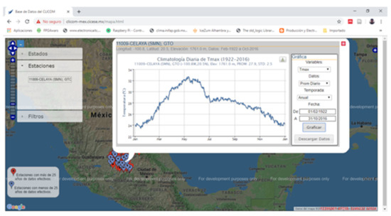
Figure 1.
Location of the weather station in Celaya, Guanajuato, Mexico.
The data were processed as a Data-Frame in Python using the Pandas library. The obtained Data-Frames presented some inconsistencies in the amount of data, as shown in Table 1. Table 2 shows descriptive statistics information for these data; descriptive statistics include those that summarize the central tendency, dispersion, and shape of the dataset’s distribution, excluding missing values. To overcome this difficulty was performed a data processing using NumPy, pandas, and Scikit-learn libraries.

Table 1.
Data amount.
Table 2.
Statistical information of the data.
It is worth mentioning that the correlation between the variables was determined to know which of them is suitable for prediction. Table 3 shows a summary of correlations, and it can be seen that only the variable “Heat” has a positive relationship of 0.8 concerning the maximum temperature variable (Max Temp).
Table 3.
Correlation matrix of the data with respect to maximum temperature.
The database was divided by the “Year”, in which the values of the variables were taken. For training, the range of years from 1922 to 2015 was used. The rest of the database (2016) was used for testing the models without loss of generality (the cross validation shown later corroborates the performance for other periods). A statistic of persistence and meteorology models was generated to compare the improvement in the proposed models, which is summarized in Table 4.
Table 4.
Results of coefficient of determination and mean square error of the persistence and weathering models.
2.2. Linear Regression Models
For model training, the maximum temperature was used as the dependent variable, taking the rest of the data such as evaporation, heat, and precipitation as independent variables.
For the linear regression calculations, given the number of variables considered and based on [30], a simple model for weather forecasting was developed. Multiple regression, quadratic and polynomial linear regression, described by the following expressions, were used:
where is the prediction of the dependent variable, the value of the independent variable and , are parameters of the equation (weights and biases).
2.3. Support Vector Machine (SVM) Model
For SVM prediction, different kernels were considered, such as linear, radial, and polynomial, and the parameter for model fitting was a penalty parameter of the error term (C):
- Linear Kernel, offers the possibility of solving problems with the approximation to a linear function.
- Kernel Polynomial, offers the possibility to solve problems with a polynomial kernel with different degrees and coefficients .
- Radial kernel, offers the possibility to solve problems with a Gaussian kernel with different values of .
- Sigmoidal kernel, offers the possibility to solve problems with a sigmoidal kernel with different and values.In the above expressions, represents the value of the line and the projection on the hyperplane, while , and are parameters of the equations. represents the scalar product of and , and represents the Euclidian norm of .
2.4. Neural Network Models
For the third prediction model, a multilayer perceptron regression neural network (MLPR), commonly used for weather forecasting (e.g., in [22]), was used. Data processing and tests with different fitting parameters are performed to reach an optimal prediction. The following are the best activation functions:
2.5. Data Scaling/Filtering
For these models, data processing was performed with minimum and maximum scaling Equation (13), L2 or Euclidean Normalization Equation (14) and standard scaling Equation (15), to perform training and verify if an improvement in the prediction of each model has been obtained:
where is an iteration index, is the number of samples, is the data, is the mean and its standard deviation.
For data processing/preparation, preliminary tests were performed using the filtering of the Data-Frame using the RANSAC algorithm to eliminate outliers and to be able to make better predictions. It should be noted that this algorithm has been widely used mainly in the adjustment for image processing (RANSAC performs a data consensus, and the set where the maximum data consensus exists are considered valid since these data are free of outliers [31,32]). It is also considered an alternative for regression, helping to eliminate noise in signals [33,34], which will help us analyze data from the smart grid’s different sensors.
From the original 34,608 records, 25,916 were left when filtered by RANSAC, as shown in Table 5.
Table 5.
Statistics of the data filtered with RANSAC.
2.6. Selection Criteria
A first criterion is used to evaluate the prediction accuracy of each model called the coefficient of determination [35]:
where are the test data, is the estimation of , , is the arithmetic mean of the data, and is the number of samples.
The mean square error result is also considered to find the best model [36]. It is worth mentioning that, contrary to the , the zero approximation improves the model’s prediction:
Finally, cross validation was performed to evaluate the prediction’s accuracy and have an advanced criterion to indicate which combination of filtering and prognosis is the best combination to predict the data.
The cross validation method consists of dividing into several data sets, one of which will be taken as the test set and the others as the training set. When performing the prediction iterations, the test set will be permuted according to the number of iterations selected to have parameters that estimate how accurate the prediction is finally.
3. Results
In this section, filtering and prediction best results, including comparative graphs, are presented.
3.1. Prediction of Maximum Temperature by Regression
Table 6 shows the best prediction parameters for the regression models with the different filtering methods, and prediction without filtering is added for comparison purposes. The results with the minimum MSE value are those considered to be the best prediction. The first column shows the data treatment used. The second column shows the type of parametrization used; it should be noted that only the most relevant results are presented due to a large number of possible combinations.
Table 6.
Training results and data testing with linear and polynomial regression predictive models.
The tests performed for linear and polynomial regression without RANSAC filtering of the data gave as best prediction results the L2 normalization and polynomial degree 7 models, the latter being the best with errors of 3.4853 and 1.9526, respectively (from the first five rows of Table 5). Figure 2a shows a comparative plot of the maximum temperature prediction results obtained from predicting without RANSAC filtering.

Figure 2.
Plot of testing and prediction data with the best linear and polynomial regression models: (a) Norm L2 and polynomial; (b) RANSAC with Norm L2 and RANSAC with polynomial.
With the RANSAC data filtering, the predictions made show a better result since the L2 normalization reached an MSE of 0.8960, which, compared to the polynomial 7-degree model, only reached 1.5190. In Figure 2b, the plot of these results concerning the original data is shown.
3.2. Maximum Temperature Prediction by Support Vector Machines
For the SVMs, the tests were also performed with different kernels to establish which one provides the best results. Table 7 shows the values of the prediction results for each model.
Table 7.
Results of training and testing data with the SVM predictive models.
It can be observed that the two best predictions in descending order without RANSAC filtering are obtained with the rbf and gamma kernels, 0.01 and 0.1, respectively. In Figure 3a, the two best prediction results concerning the original data are illustrated. On the other hand, with RANSAC filtering again, considerable improvements in MSE are obtained. With standard scale, kernel = rbf, C = 1000, gamma = 0.1 we obtain an 1.1508 MSE. Figure 3b shows the two best results obtained from the prediction with the RANSAC filtered data compared to the original test data.
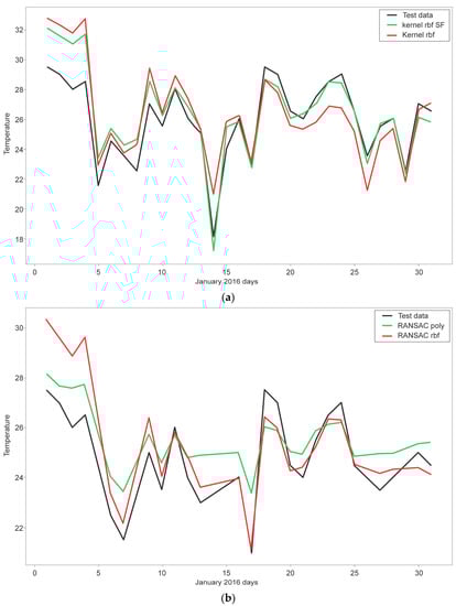
Figure 3.
Plot of the prediction of the original data with respect to the prediction with SVM models: (a) Kernel rbf SF and Kernel rbf; (b) RANSAC polynomial and rbf.
3.3. Maximum Temperature Prediction by Neural Networks
For the MLPR model, Table 8 shows the results obtained from the prediction with different parameterizations. In this case, the best MSE without RANSAC filtering is obtained with standard scaling, while the best work is again with RANSAC filtering and standard scaling. In Figure 4a, the two best results without RANSAC filtering are illustrated, and in Figure 4b, the two best results with RANSAC filtering are shown.
Table 8.
Results of training and testing data with the neural network predictive models.

Figure 4.
Plot of the prediction of the original data with respect to the prediction with MLPR models: (a) tanh and ReLU activations; (b) Norm L2 and polynomial.
3.4. Cross Validation
From the statistics shown in Section 3.1 to Section 3.3, it can be observed that better results for MSE and are obtained by using the RANSAC filtering, and considerable improvement in the prediction can be reached.
A cross validation of the results was performed to get a reliable final decision and shown in Figure 5. The best model is undoubtedly predicting using RANSAC filtering and standard scale, which surpasses the previous models obtaining a higher accuracy in the confidence interval. It should be noted that a parameterization of K-fold = 10 was used, and a random error of ±0.05 was obtained in the best case.
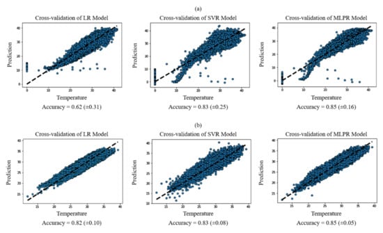
Figure 5.
Cross validation for: (a) the prediction of unfiltered and unscaled data; (b) RANSAC-filtering.
3.5. Prediction of Energy Conditions
To strengthen this study, we added the Watts per hour that were consumed in a household. The additional data for this prediction were obtained from [37] (household_power_consumption.zip), from which the date and consumed Watts per hour were extracted to match (in time and geographic zone) the data in the previously treated database.
Figure 6 compares the predictions with the three models, highlighting that the neural networks, although they give a prognosis similar to the linear regression, improve the error rate. It should be noted that the amount of training data was much smaller, and even so, the results obtained in previous sections are confirmed.
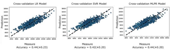
Figure 6.
Cross validation of energy data prediction with RANSAC filtering.
4. Discussion
One of the main tasks to achieve an adequate prediction of the relevant variables for an energy management strategy in a smart grid is treating the data. In this paper, it can be seen that the results change significantly depending on the type of data filtering/scaling, and the results show that such treatment is essential. Standard scaling (in Python Standar Scaler) provided the best results for support vector machines and neural networks.
The result of the coefficient of determination was better in support machines and neural networks as opposed to polynomial regression. Although the lowest MSE was obtained by the latter method, it could be supported that the networks improve the model by cross validation, in which a clear prediction improvement is distinguished for neural networks as opposed to the other models.
It is worth mentioning that this paper did not present the results of each combination of filtering and prediction but only the best ones and that each combination can take hours or even days to yield results.
Although linear regression models are simple models, they generate good results in prediction only if the appropriate data treatment is performed.
On the other hand, the measurement of variables includes noise and even erroneous sampling by exogenous conditions, such as human errors and accidental modification of the sensing environment.
Commonly, predictive energy management strategies for smart grids need accurate data predictions. Indeed, it is rarely studied an appropriate signal-filtering for predicting the dynamic behavior of the grid’s variables as temperature, power consumption, voltage, and many others, by neural networks.
Remarkably, the RANSAC algorithm with L2 Norm for filtering the measured variables is a novelty. Even more, the prediction by combining an MLPRNN provides better forecasts. From the proven combinations of neural networks, filtering, and scaling, this was the combination that best results that provided in R2, MSE, and cross validation terms. Unlike other studies that compare data prediction accuracy for a smart grid, this paper includes a cross validation to indicate whether there are overfitting or selection bias problems, not to mention that it does not include comparative analysis of filtering techniques.
5. Conclusions
From the results obtained in the predictive models and filtering techniques presented, first of all, the advantage of processing the data to improve the prediction considerably should be highlighted. The RANSAC outlier filtering reduces the error and yields prediction values that are better adjusted to the real values. Thus, it can be deduced that it is possible to predict meteorological variables and energy behaviors associated with the smart grid acceptably. Using RANSAC filtering and standard scale, the multilayer perceptron regression neural network is the best combination of those tested in this study.
It should be taken into account that others can substitute the database and the prediction variables. In this study, the temperature was used as a case study, in addition to the electric power demand for prediction.
As future work, deep learning neural networks for prediction should be considered since they have become popular for their improvement in the adjustment of nonlinear data, such as the data set analyzed in this work. Besides, databases appropriate to the variable of interest to be predicted should be proposed.
Author Contributions
Conceptualization, M.A.R.-L. and H.R.-G.; methodology, M.A.R.-L. and E.E.-A.; software, E.E.-A.; validation, M.A.R.-L., H.R.-G. and E.E.-A.; formal analysis, M.A.R.-L. and E.E.-A.; investigation, E.E.-A.; resources, M.A.R.-L. and E.E.-A.; data curation, E.E.-A.; writing—original draft preparation, M.A.R.-L., H.R.-G., A.G.S.-S., F.J.P.-P. and E.E.-A.; writing—review and editing, M.A.R.-L., A.G.S.-S., F.J.P.-P. and H.R.-G.; visualization, E.E.-A.; supervision, M.A.R.-L. and H.R.-G.; project administration, M.A.R.-L.; funding acquisition, M.A.R.-L. and F.J.P.-P. All authors have read and agreed to the published version of the manuscript.
Funding
This research was funded by CONACYT, grant number Cátedras CONACYT 4155 and the scholarship of E.E.-A.
Institutional Review Board Statement
Not applicable.
Informed Consent Statement
Not applicable.
Data Availability Statement
Data used in this research are freely available from the following site: http://clicom-mex.cicese.mx/ (accessed on 1 April 2021).
Conflicts of Interest
The authors declare no conflict of interest.
References
- Craparo, E.; Karatas, M.; Singham, D.I. A robust optimization approach to hybrid microgrid operation using ensemble weather forecasts. Appl. Energy 2017, 201, 135–147. [Google Scholar] [CrossRef]
- Mattig, I.E. Predicción de la Potencia Para la Operación de Parques Eólicos; Universidad de Chile: Santiago, Chile, 2010. [Google Scholar]
- Agüera-Pérez, A.; Palomares-Salas, J.C.; de la Rosa, J.J.G.; Florencias-Oliveros, O. Weather forecasts for microgrid energy management: Review, discussion and recommendations. Appl. Energy 2018, 228, 265–278. [Google Scholar] [CrossRef]
- Cecati, C.; Mokryani, G.; Piccolo, A.; Siano, P. An overview on the smart grid concept. In Proceedings of the IECON 2010-36th Annual Conference on IEEE Industrial Electronics Society, Glendale, AZ, USA, 7–10 November 2010; pp. 3322–3327. [Google Scholar]
- Kadlec, M.; Bühnová, B.; Tomšík, J.; Herman, J.; Družbíková, K. Weather forecast based scheduling for demand response optimization in smart grids. In Proceedings of the 2017 Smart Cities Symposium Prague, SCSP 2017-IEEE Proceedings, Prague, Czech Republic, 25–26 May 2017; pp. 1–6. [Google Scholar]
- Wan, C.; Zhao, J.; Song, Y.; Xu, Z.; Lin, J.; Hu, Z. Photovoltaic and solar power forecasting for smart grid energy management. CSEE J. Power Energy Syst. 2016, 1, 38–46. [Google Scholar] [CrossRef]
- Sarwat, A.I.; Amini, M.; Domijan, A.; Damnjanovic, A.; Kaleem, F. Weather-based interruption prediction in the smart grid utilizing chronological data. J. Mod. Power Syst. Clean Energy 2016, 4, 308–315. [Google Scholar] [CrossRef]
- Bansal, A.; Rompikuntla, K.; Gopinadhan, J.; Kaur, A.; Kazi, Z.A. Energy Consumption Forecasting for Smart Meters. In Proceedings of the International Conference on Business and Information, BAI 2015, Cotai, Macao, 3–4 July 2014; pp. 1–20. [Google Scholar]
- Hernández, L.; Baladrón, C.; Aguiar, J.M.; Calavia, L.; Carro, B.; Sánchez-Esguevillas, A.; Cook, D.J.; Chinarro, D.; Gómez, J. A study of the relationship between weather variables and electric power demand inside a smart grid/smart world framework. Sensors 2012, 12, 11571–11591. [Google Scholar] [CrossRef]
- Calanca, P.; Bolius, D.; Weigel, A.P.; Liniger, M.A. Application of long-range weather forecasts to agricultural decision problems in Europe. J. Agric. Sci. 2011, 149, 15–22. [Google Scholar] [CrossRef]
- Kavitha, R.; Anuvelavan, M.S. Weather MasterMobile Application of Cyclone Disaster Refinement Forecast System in Location Based on GIS Using Geo Algorithm. Int. J. Sci. Eng. Res. 2015, 6, 88–93. [Google Scholar]
- Hasan, N.; Nath, N.C.; Rasel, R.I. A support vector regression model for forecasting rainfall. In Proceedings of the 2nd International Conference on Electrical Information and Communication Technologies, EICT 2015, Khulna, Bangladesh, 10–12 December 2015; pp. 554–559. [Google Scholar]
- Ngeleja, R.C.; Luboobi, L.S.; Nkansah-Gyekye, Y. The Effect of Seasonal Weather Variation on the Dynamics of the Plague Disease. Int. J. Math. Math. Sci. 2017, 2017, 1–25. [Google Scholar] [CrossRef]
- Bouza, C.N.; Garcia, J.; Santiago, A.; Rueda, M. Modelos Matemáticos Para el Estudio de Medio Ambiente, Salud y Desarrollo Humano (TOMO 3), 1st ed.; UGR: Granada, Spain, 2017. [Google Scholar]
- Les, U.D.E.; Balears, I.; Doctoral, T. Redes Neuronales Artificiales Aplicadas al Análisis de Datos; Universitat de les Illes Balears: Illes Balears, Spain, 2002. [Google Scholar]
- Sobhani, M.; Campbell, A.; Sangamwar, S.; Li, C.; Hong, T. Combining Weather Stations for Electric Load Forecasting. Energies 2019, 12, 1510. [Google Scholar] [CrossRef]
- Vincenti, S.S.; Zuleta, D.; Moscoso, V.; Jácome, P.; Palacios, E. Análisis Estadístico de Datos Metereológicos Mensuales y Diarios Para la Determinación de Variabilidad Climática y Cambio Climático en el Distrito Metropolitano de Quito. La Granja 2012, 16, 23–47. [Google Scholar] [CrossRef]
- Jacobson, T.; James, J.; Schwertman, N.C. An example of using linear regression of seasonal weather patterns to enhance undergraduate learning. J. Stat. Educ. 2009, 17, 2009. [Google Scholar] [CrossRef][Green Version]
- Gupta, S.; Singhal, G. Weather Prediction Using Normal Equation Method and Linear regression Techniques. Int. J. Comput. Sci. Inf. Technol. 2016, 7, 1490–1493. [Google Scholar]
- Mori, H.; Kanaoka, D. Application of support vector regression to temperature forecasting for short-term load forecasting. In Proceedings of the IEEE International Conference on Neural Networks-Conference Proceedings, Orlando, FL, USA, 12–17 August 2007; pp. 1085–1090. [Google Scholar]
- Radhika, Y.; Shashi, M. Atmospheric Temperature Prediction using Support Vector Machines. Int. J. Comput. Theory Eng. 2009, 55–58. [Google Scholar] [CrossRef]
- Narvekar, M.; Fargose, P. Daily Weather Forecasting using Artificial Neural Network. Int. J. Comput. Appl. 2015, 121, 9–13. [Google Scholar] [CrossRef]
- Ali, J.; Kashyap, P.S.; Kumar, P. Temperature forecasting using artificial neural networks. J. Hill Agric. 2013, 4, 110–112. [Google Scholar]
- Paisan, Y.P.; Moret, J.P. La Repetibilidad Y Reproducibilidad En El Aseguramiento De La Calidad De Los Procesos De Medición. Tecnol. Química 2010, 2, 117–121. [Google Scholar]
- De Almeida, C.T.; Galvão, L.S.; Aragão, L.E.d.C.e.; Ometto, J.P.H.B.; Jacon, A.D.; de Souza Pereira, F.R.; Sato, L.Y.; Lopes, A.P.; de Alencastro Graça, P.M.L.; de Jesus Silva, C.V.; et al. Combining LiDAR and hyperspectral data for aboveground biomass modeling in the Brazilian Amazon using different regression algorithms. Remote Sens. Environ. 2019, 232, 111323. [Google Scholar] [CrossRef]
- Jahromi, K.G.; Gharavian, D.; Mahdiani, H. A novel method for day-ahead solar power prediction based on hidden Markov model and cosine similarity. Soft Comput. 2019. [Google Scholar] [CrossRef]
- Raffán, L.C.P.; Romero, A.; Martinez, M. Solar energy production forecasting through artificial neuronal networks, considering the Föhn, north and south winds in San Juan, Argentina. J. Eng. 2019, 2019, 4824–4829. [Google Scholar] [CrossRef]
- Valappil, V.K.; Temimi, M.; Weston, M.; Fonseca, R.; Nelli, N.R.; Thota, M.; Kumar, K.N. Assessing Bias Correction Methods in Support of Operational Weather Forecast in Arid Environment. Asia Pac. J. Atmos. Sci. 2019, 56, 333–347. [Google Scholar] [CrossRef]
- CICESE. Datos Climáticos Diarios Del CLICOM Del SMN a Través de su Plataforma Web Del CICESE. 2018. Available online: http://clicom-mex.cicese.mx/ (accessed on 19 May 2019).
- Mathur, S. A Simple Weather Forecasting Model Using Mathematical Regression. Indian Res. J. Ext. Educ. 2012, I, 161–168. [Google Scholar]
- Foley, J.D.; Fischler, M.A.; Bolles, R.C. Graphics and Image Processing Random Sample Consensus: A Paradigm for Model Fitting with Applications to Image Analysis and Automated Cartography. Commun. ACM 1981, 24, 1–15. [Google Scholar]
- Yaniv, Z. Random Sample Consensus (RANSAC) Algorithm, A Generic Implementation. Insight J. 2010, I, 1–14. [Google Scholar]
- Djurović, I. QML-RANSAC: PPS and FM signals estimation in heavy noise environments. Signal Process. 2017, 130, 142–151. [Google Scholar] [CrossRef]
- Choi, S.; Kim, T.; Yu, W. Performance Evaluation of RANSAC Family. DBLP 2009. [Google Scholar] [CrossRef]
- Scikit-Learn.org. r2 Score. Available online: https://scikit-learn.org/stable/modules/model_evaluation.html#r2-score (accessed on 27 March 2021).
- Scikit-Learn.org. Mean Squared Error. Available online: https://scikit-learn.org/stable/modules/model_evaluation.html#mean-squared-error (accessed on 27 March 2021).
- UCI Machine Learning Repository: Individual Household Electric Power Consumption Data Set. Available online: https://archive.ics.uci.edu/ml/datasets/individual+household+electric+power+consumption# (accessed on 10 November 2020).
Publisher’s Note: MDPI stays neutral with regard to jurisdictional claims in published maps and institutional affiliations. |
© 2021 by the authors. Licensee MDPI, Basel, Switzerland. This article is an open access article distributed under the terms and conditions of the Creative Commons Attribution (CC BY) license (https://creativecommons.org/licenses/by/4.0/).