Article

Experimental Study of the Use of Tracing Particles for Interface Tracking in Primary Cementing in an Eccentric Hele–Shaw Cell

1
Department of Geoscience and Petroleum, NTNU, S. P. Andersens vei 15A, 7031 Trondheim, Norway
2
SINTEF Industry, S.P. Andersens vei 15B, 7031 Trondheim, Norway
*
Author to whom correspondence should be addressed.
Energies 2021, 14(7), 1884; https://doi.org/10.3390/en14071884
Submission received: 1 February 2021 / Revised: 11 March 2021 / Accepted: 20 March 2021 / Published: 29 March 2021
(This article belongs to the Special Issue Recent Advances in Petroleum Drilling Engineering)

Abstract

:
We present the results of the displacement flows of different Newtonian and Herschel–Bulkley non-Newtonian fluids in a new-developed eccentric Hele–Shaw cell with dynamic similarly to real field wellbore annulus during primary cementing. The possibility of tracking the interface between the fluids using particles with intermediate or neutral buoyancy is studied. The behaviors and movements of particles with different sizes and densities against the primary vertical flow and strong secondary azimuthal flow in the eccentric Hele–Shaw cell are investigated. The effects of fluid rheology and pumping flow rate on the efficiency of displacement and tracing particles are examined. Moreover, the behavior of pressure gradients in the cell is described and analyzed. Successful results of tracing the interface using particles give us this opportunity to carry out a primary cementing with high quality for the cases that the risk of leakage is high, e.g., primary cementing in wells penetrating a CO2 storage reservoir.

1. Introduction

One of the essential operations during the drilling of oil and gas wells is the primary cementing of the wellbore annulus and the displacement of the drilling fluid and formation fluids in the annulus. The procedure of this operation involves pumping non-Newtonian yield-stress fluids of progressively higher density and rheology into the wellbore annulus, spacers with higher density and rheology than drilling fluids, and subsequently cements with higher density and rheology than the other existing fluids in the annulus. This successive pumping causes stabilizing the displacement process and the interfaces between the fluids in the annulus and increases displacement efficiency and well integrity [1,2]. Numerous factors result in imperfect displacement and low-quality cementing, e.g., uneven borehole due to soft rocks and washouts and eccentric positioning of the casing within the borehole, which causes the nonuniform advance of fluid interfaces in the wellbore annulus and bypassing of the pockets or channels of mud/spacer along it [3].
There are numerous numerical and experimental studies of the displacement flows of Newtonian and non-Newtonian fluids in annular geometries. Due to the problematic rheological behaviors of non-Newtonian fluids with and without yield-stress, there are fewer experimental studies about fluid flows in concentric and eccentric annular geometries with similarity to wellbore annulus in primary cementing [4,5,6,7,8,9,10,11,12,13,14,15,16]. In these limited experimental studies, it has been established that the type of flow (laminar, transition, and turbulent) [5,10,11,12,17,18] and degree of eccentricity affect displacement efficiency significantly [19]. These studies generally stated that turbulent displacement flow is more efficient than the laminar displacement flow [17,18], and the increasing standoff causes a significant effect on the displacement flow of the fluids and cement placement [20,21,22]. In cases like washout sections, the effect of inner pipe eccentricity is not significant for displacement in the washout section [23]. Moreover, inclination reduction is beneficial for the displacement efficiency within the hole enlargement for both concentric and eccentric annuli and in the regular part of the annulus in front of the enlargement [22]. Furthermore, the effects of viscous and buoyancy forces [5] and the rotation of the inner cylinder [6,7,13] on the annular displacement process were emphasized. The effects of gravity-driven azimuthal flow or secondary flow triggered due to the different fluid interface levels in the annulus’ wide and narrow sections on improving the displacement flow process and simultaneously trapping pockets of displaced fluid on the narrow side were described [4,8,9]. The frictional pressure drop and the relation between pressure drop and flow rate during the displacement flow of non-Newtonian fluids were described as well [4,10,11]. By using large-scale eccentric annular geometry, the importance of the rheological properties of the realistic non-Newtonian fluids for fluid flow and hole cleaning performance was expressed extensively [14,15,16], and the propagation of the fluid interfaces and displacement efficiency were characterized [24]. It was indicated that an enlarged irregular section, i.e., a washout causes an improvement in displacement in some scenarios in strongly inclined wellbores [17]; while being independent of the displacement efficiency in the washout itself, the presence of washouts may lead to poorer cement quality downstream of the washouts [23].
An alternate methodology for studying the annular displacement flow is neglecting the local curvature of the annulus and unwrapping it into a Hele–Shaw cell with a varying gap through the width of the cell to represent an eccentric annulus [25,26,27,28]. It has been proven that this assumption is valid when the ratio of the inner radius and the outer radius of the annulus is larger than 0.3 (ri/ro ≥ 0.3) [29]. Moreover, a CFD analysis validates using Hele–Shaw cell geometries instead of annular geometry for more accurate and detailed studies of the displacement laminar flow tests, by qualitative and quantitative comparison of an eccentric annular model and an equivalent Hele–Shaw model [30]. This approach was implemented for numerical modeling and analytical solutions of concentric and eccentric wellbore annular geometries for the study and more accurate observation of displacement flow during primary cementing and mud removal in an oil well [25,26,27,28]. A Hele–Shaw cell with a constant gap mimicking a vertical section of a concentric wellbore annulus was used for vertical displacement flow of Newtonian and Herschel–Bulkley non-Newtonian fluids, and displacement stability and efficiency, viscous fingering and bypassing pockets of displaced yield-stress fluid in displacing fluid has been investigated experimentally [31].
Several solutions exist in real field operations for evaluating the displacement efficiency and quality of primary well cementing, like cement bond log (CBL) and temperature logs. However, there is still a lack of an approach to check the cement column quality during operation and show the presence of voids or mud pockets, required mainly in wells penetrating CO2 storage reservoirs where the leakage of CO2 is a crucial parameter [32]. For these wells, all annular cement columns must be of a high quality due to the buoyancy of CO2 and because these wells are exposed to harsh conditions, e.g., the cooling of the well/formation, elevated pressure, and chemical reactions [3]. A recently introduced approach for identifying the location of the interface between successive fluids in a wellbore annulus (e.g., cement–spacer or spacer–mud) is by using tracing particles; particles with intermediate buoyancy that remain at the interfaces between successive fluids or tagging one of the fluids with neutrally buoyant particles [30,31,33,34,35]. The essential active forces in these situations are drag and buoyancy forces, competing with each other. The drag force causes the particle to move at the local fluid velocity, while the buoyancy force attracts the particles where it is zero. The tracing particles must dominate over azimuthal secondary flows to indicate the interface precisely [34]. This approach has been approved numerically by solving the Hele–Shaw model and involving the particles in the models with Newtonian and non-Newtonian fluids [33,34]. Intermediate buoyant particles have been employed for interface tracking in concentric and eccentric experimental annular geometries, and their effectiveness in different cell inclinations and by using different fluid rheology and displacement flow rates were explored [30,35]. Moreover, the use of intermediate buoyant particles for tracking the interface of stable and unstable displacement flows has been examined successfully using an experimental Hele–Shaw cell geometry with a uniform gap representing a concentric wellbore annulus [31].
In this study, the previously developed concentric Hele–Shaw cell with dynamic similarity to real field wellbore annulus during primary cementing [31] was upgraded to a Hele–Shaw cell which mimics a displacement flow in an “eccentric” annulus geometry. To the best of our knowledge, only the use of Hele–Shaw cells with uniform gaps has been reported in the literature to investigate different flow mechanisms, and this is the first experimental Hele–Shaw cell study with a nonuniform gap. Several displacement flow tests at different flow rates were performed using the upgraded cell and different pairs of Newtonian and Herschel–Bulkley non-Newtonian fluids. The efficiency of the displacement and the shape of the interface between the successive pumped fluids and the applications of particles with different sizes and densities for tracking the interface between these two fluids are examined. The particles can be placed on the interface between the fluids or can be immersed in one of the fluids. The effect of secondary azimuthal flow in the eccentric annuli on the interface shape and behavior of the tracing particles are studied. The recorded pressure gradients in the cell are analyzed as well.

2. Experimental Design and Procedure

The eccentric Hele–Shaw cell used in this study is an upgrade of the previously used concentric Hele–Shaw cell, the full experimental description of which was described elsewhere in detail [31]. Here, a summary of the experimental design, experimental setup and procedure, fluid property and measurements is reviewed, and the characteristic of the new upgraded eccentric Hele–Shaw cell is described in more detail.
As described before on dynamic similarity of displacement flow in the concentric geometries with real field conditions [31], the aspect ratio of the circumferential and radial length scales (δ), experimental Reynolds and Buoyancy numbers are the main flow-controlling parameters that should be considered in addition to eccentricity in eccentric geometries. The degree of the casing eccentricity in the wellbore is usually described by the standoff, as follows:
s t a n d o f f %   =   1 d r o r i × 100
where in these equations, ro, ri, and d are the outer radius of the annulus, the inner radius of the annulus, and the distance between the casing and wellbore centers, respectively. The definition of the aspect ratio of circumferential and radial length scales (δ), experimental Reynolds (Re) and Buoyancy (Bu) numbers are as follows:
δ   =   ( r o r i ) / π r o + r i
R e i   =   2 ρ i w ¯ h μ e i
B u   =   Δ ρ g h 2 w ¯ μ e 2
The subscripts i = 1 and 2 refer to the displaced and displacing fluids, respectively. Here, µe is a representative effective viscosity that is simply evaluated by µe = τ(γ·e)/γ·e using an effective shear rate (γ·e) given by γ· e = 4 w ¯ / h . w ¯ and h are the mean flow velocity and the mean gap in the annulus, respectively [8,9,12].
The first step for designing an experiment is downscaling real well data (in the second row of Table 1) with a ratio of 0.25 and replacing the density and rheology of the fluids used in the lab (related data to test no. 6 that will be discussed later) in the calculations of the dimensionless parameters of the downscaled annular geometry, as shown in the third row of Table 1. In the downscaled geometry, the aspect ratio of length and width scales (η = l/h) of 100 was found to be good to produce a fully developed laminar flow, while it is much smaller than a typical value of the real cemented annulus. The aspect ratio of the circumferential and radial length scales (δ) is in the range of the field values. The dimensionless numbers were calculated by assuming the mean flow velocity of 0.1 m/s. The Reynolds number for the scaled model shows that the displacement flow is fully laminar, and the Buoyancy number is at the same order of magnitude as the above-reported field values [8,9] and in the typical range of the existing experimental studies in this area in the literature [12].
As the radius ratio is ri/ro = 0.81 ≥0.3, it is acceptable to unwrap the annulus into a Hele–Shaw cell [14]. By assuming a standoff of 60% equivalent to 0.004 m distance between the casing and wellbore centers (d) (by using Equation (1)), the width and the variation of the gap by the width in the equivalent Hele–Shaw cell are calculated using Equations (5) and (6). The gap of the Hele–Shaw cell representing the annular width at a given polar angle θ is defined as the distance between the casing and the wellbore contours measured along the casing radius. It is expressed as follows:
h   =   d c o s y r * + r o 1 d r o 2 s i n 2 y r * r i , y π r * , π r *
where h, and y are the gap, and the width, respectively. r* is given by:
r *   =   π r o 2 π r i 2 4 r o E d / r o 2 π r i
where E(x) is the elliptic integral of the second kind [30]. The width of the Hele–Shaw cell is calculated as 2πr*, which is 0.3 m here. The calculated variation of the gap by the width of the cell can be seen in Figure 1 for a 0.6-m width that is double the calculated width for removing the boundary effects. As shown in this figure, the minimum and maximum gaps are 6 mm and 14 mm, respectively, and the cross-sectional area of the cell is 0.006 m2. The 0.3-m width in the middle section of the model is the main section of analysis without any probable boundary effects. The length of the model is 1 m, and the real pump rate in the lab will be 6 × 10⁻⁴ m3/s, which is twice the calculated pump rate in Table 1 (3 × 10⁻⁴ m3/s) for achieving a mean flow velocity of 0.1 m/s.
This gap variation is machined on a 50 mm thick acrylic plate, which stands against a flat acrylic plate using a stainless-steel spacer, as shown in Figure 2. Six inlet and six outlet ports, and six 1/4-inch ports at a distance of 10 cm above the bottom of the cell and for releasing particles into the cell were designed.
The experimental setup consists of two centrifugal pumps for pumping displacing and displaced fluids into the cell, a variable frequency drive to adjust the displacing fluid flow rate, a Heinrichs magnetic flow meter, two GE Druck pressure transmitters, and a Fuji differential pressure transmitter. The ports of the pressure transmitters were placed in spaces with a depth of 15 mm, length of 600 mm, and width of 15 mm (more than 10 mm average gap in the main body of the cell), as shown by the color red in Figure 2a. The pumped fluids are spread in these spaces before arriving in the cell and leaving it. During the displacement flow tests, the bottom and top transmitters are in contact with the displacing and displaced fluids, respectively. The whole setup is in Figure 3. The Hele–Shaw cell is in a vertical direction for performing the tests, and the flow is in the vertical direction from the bottom to the top. A displaced fluid first fills the cell from the bottom. This fluid is then displaced with a displacing fluid with a higher density and viscosity from the bottom to a specified height below the particle release-ports and with a very small flow rate to have a flat interface between the two fluids. Subsequently, the particles are released into the cell in the displaced fluid using syringes filled with the particles. The particles are released in the displaced fluid with lower density and viscosity to have more opportunity to immerse them on the interface. The interface is then moved slowly to a height of 20 cm from the bottom of the cell. This is the initial status of the interface for the start of the tests. The experiment starts by pumping the displacing fluid from the bottom into the cell. The flow rate, pressures at the inlet, and outlet and pressure differences are logged on a PC, and images of the displacement process are recorded using a Canon EOS 5D Mark IV camera at one-second intervals.
Several pairs of Newtonian and non-Newtonian fluids are prepared and used in this series of experiments. Water and aqueous sucrose solution as Newtonian fluids and neutralized Carbopol-980 solutions at an intermediate pH value (using NaOH) as non-Newtonian fluids with shear-thinning and yield-stress behavior are used in this study. Brilliant Cresyl Blue was added to the displaced fluids for visualization purposes [36], sucrose was used as a weighting agent to increase the Carbopol solution density, and NaCl was added to increase electrical conductivity. Fluid densities and pHs were measured in the lab, and the rheological properties of the fluids were measured before each test using an Anton Paar MCR 102 rheometer at a fixed temperature of 21 °C. The rheology data were fitted to a Herschel–Bulkley model, τ   =   τ y + κ γ ˙ n , where n is the power-law index, κ is the consistency index, and τy is the yield-stress. Table 2 presents an overview of compositions, pH, and density of the displaced and displacing fluids in the tests.
Table 3 shows the properties of the fluids used in the tests. Subscripts 1 and 2 are representative of displaced and displacing fluids, respectively. The rheology data have been extracted from shear stress vs. shear rate plots shown in the following sections.
Table 4 shows the names and properties of the particles that we have used.

3. Experimental Results and Discussion

3.1. Experimental Overview

We completed nine tests in the eccentric Hele–Shaw cell using different pairs of Newtonian and non-Newtonian fluids, particle sizes, flow rates, and effective shear rates, as shown in Table 5. The calculated Reynolds number based on the displacing fluid ranges from 0.98 in tests with two non-Newtonian fluids to 369.3 in the tests with two Newtonian fluids showing fully laminar displacement flows. The range of the buoyancy number is from 1.69 in the tests with two non-Newtonian fluids to 924.49 in the tests with two Newtonian fluids. In the most similar tests to a real primary cementing operation (tests no. 6 to 9 with two non-Newtonian fluids with yield-stress), the buoyancy numbers are in the same order of magnitude as the reported values [8,9].

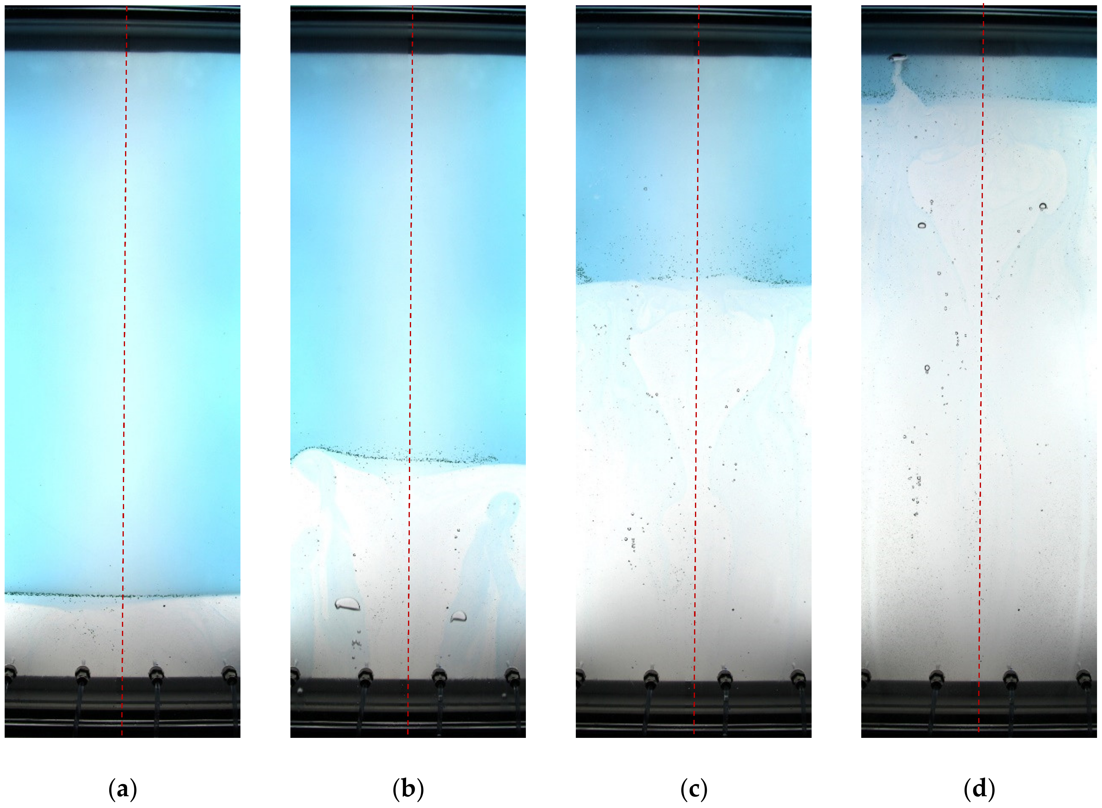
3.2. Displacement Flow Tests 1 and 2: Newtonian Fluids

In this section, the snapshots of fluid displacement in the eccentric Hele–Shaw cells are presented, and the use and effectiveness of particles for tracking the interface between the displaced and displacing fluids are described. The rheological properties of the displaced and displacing fluids are reviewed and discussed. Moreover, the pressure drop values in the tests are described and analyzed. We consider a middle section of the model with a width of 30 cm for analyzing snapshots of the displacement flow, as we discussed before, to remove edge boundary effects. We have marked the narrowest part of the cell by a dashed red centerline in the middle of the cell, and the left and right-hand sides of this line are the widest sides.
In tests no. 1 and 2, both displaced and displacing fluids have Newtonian behavior; water with a density of 1.00 g/cc and a viscosity of 9.56 × 10⁻⁴ Pa·s as displaced, and 35 wt/wt% sucrose solution with a density of 1.15 g/cc and a viscosity of 3.17 × 10⁻³ Pa·s as displacing fluid. We used particles with diameters of 3000 (no. 3) and 1000 µm (no. 2) in tests no. 1 and 2, respectively. After initializing the cell, the main displacement flows are started with the recorded flow rate rates of 18.06 L/min and 18.28 L/min in tests no. 1 and 2, respectively. In these two tests, the released particles remain on the interface after release. Figure 4 and Figure 5 show snapshots of the displacement flows in these two tests. We can see stable and pistonlike displacement that verifies a strong secondary azimuthal flow in these two tests, mainly due to the small fluid viscosities. In test no. 1, we can see a little movement of the particles from the wide side to the narrow side on the right-hand side of the cell and simultaneously from the narrow side to the wide side on the left-hand side of the cell. This means that the particles on the right-hand side of the cell may be influenced by the secondary flow in the displacing fluid from the wide side to the narrow side, while the particles on the left-hand side of the cell may be affected by the secondary flow in the displaced fluid in this section. While there is a symmetry in the cell, two opposite effects are observed on two sides of the cell. It shows the importance of the particle locations (above or below the interface) to know which secondary flows, in the displaced or displacing fluid, affect them. In test no. 2, we do not see any considerable movement of particles through the width of the model by comparing the concentration of particles over time in Figure 5, and it can be expressed that the interface is appropriately tracked using these particles. Additionally, it confirms that the negligible movements of particles in test no. 1 are because of the particle interactions and not the secondary flows in the fluids.

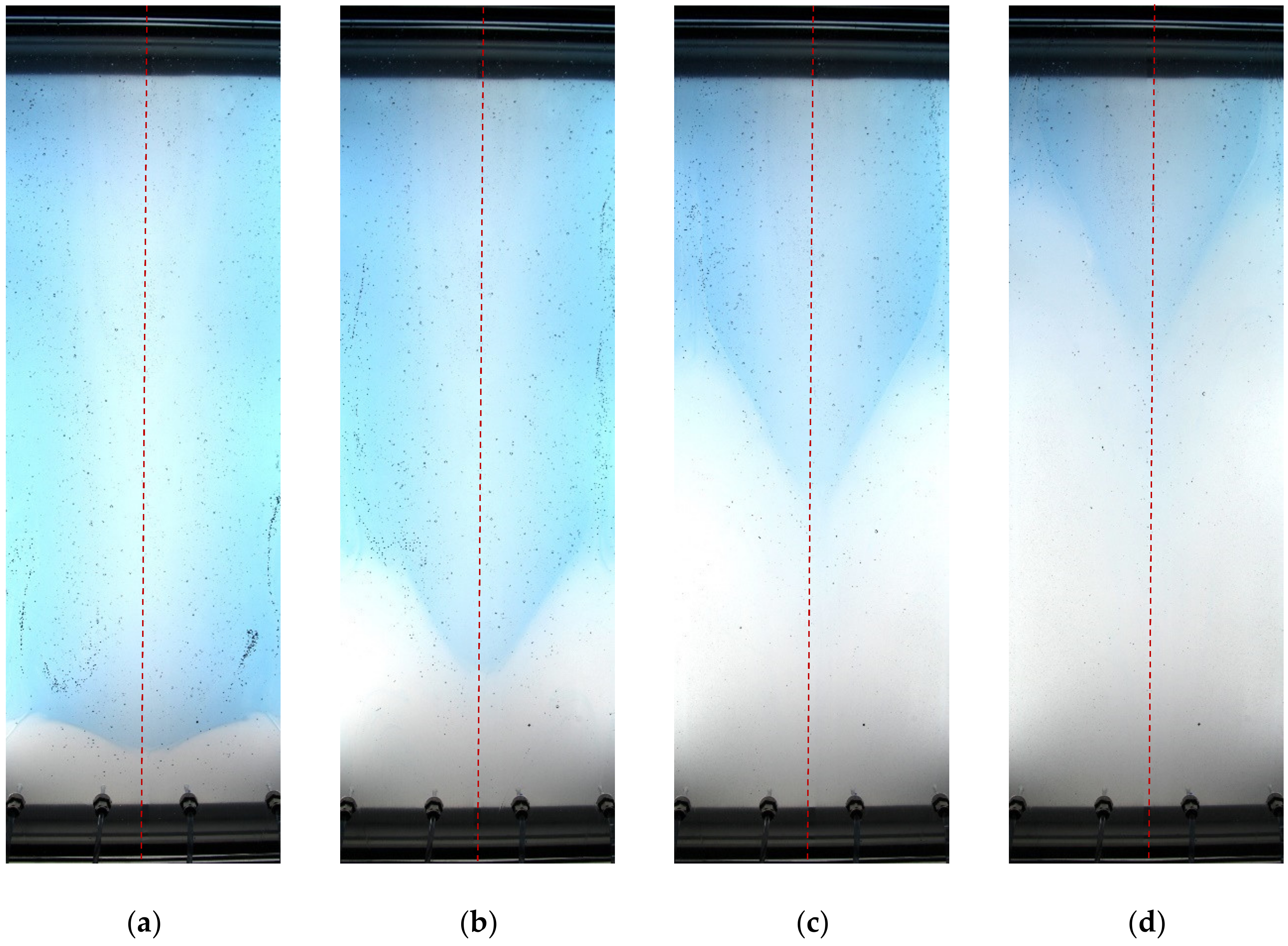
3.3. Displacement Flow Tests 3 to 5: Newtonian/Non-Newtonian Fluids

In tests no. 3, 4, and 5, the displaced and displacing fluids are water with a density of 1.00 g/cc, and carbopol and sucrose solution with a density of 1.15 g/cc, respectively. Figure 6 shows the rheological behavior and viscosity of the displaced and displacing fluids and the range of the effective shear rates in these three tests. It confirms the Newtonian behavior of the displaced fluid with a viscosity of 9.558 × 10⁻⁴ Pa·s, and non-Newtonian behavior of the displacing fluid with a yield stress of 1.33 Pa and considerably higher equivalent viscosity compared to the displaced fluid. Therefore, the displacing fluid has higher density and viscosity than the displaced fluid. Particles with diameters of 1000 (no. 2), 3000 (no. 3), and 850 µm (no. 1) and displacement flow rates of 15.27, 22.86, 22.17 L/min are used in tests no. 3, 4, and 5, respectively. For the initialization of the tests, the same procedure as before is applied.
In Figure 7, Figure 8 and Figure 9 showing the snapshots of the displacement flows in these three tests, we see almost pistonlike and stable displacements. The interfaces between the fluids in these tests are not entirely flat, confirming the existence of a weaker azimuthal secondary flow than tests no. 1 and 2 due to the higher equivalent viscosity of the displacing fluids here. The lower flow rate in test no. 3 causes a flatter interface due to the lower displacement flow rate and higher secondary flow. Figure 7 shows that the 1000-µm particles move from the wide sides to the narrow side and accumulate on the narrowest side of the cell due to the secondary flow in the displacing fluid. On this side, most of the particles travel toward the top of the cell with the same velocity as the interface and track the interface. Some particles bypass the interface on the narrow side and move toward the top with a lower velocity than the interface. Figure 8 shows slight movements of the 3000-µm particles from the narrow side to the wide side on the right-hand side of the cell and from the wide side to the narrow side on the left-hand side of the cell. While it seems that the particles are located in the displaced fluid and affected by the secondary flow there, their movements toward the narrow section on the left-hand side of the cell are not reasonable. The particles’ interactions on each other could be a reason for the movement of particles in this test and on both sides of the cell, and it seems that these particles overcome the secondary flow in this test. The displacement flow in test no. 5 is disturbed by the air bubbles, as can be seen in Figure 9. However, it can be seen in this figure that the particles with the size of 850 µm move from the narrow side to the wide side because they are under the influence of the secondary flow in the displaced fluid from the narrow side to the wide side.

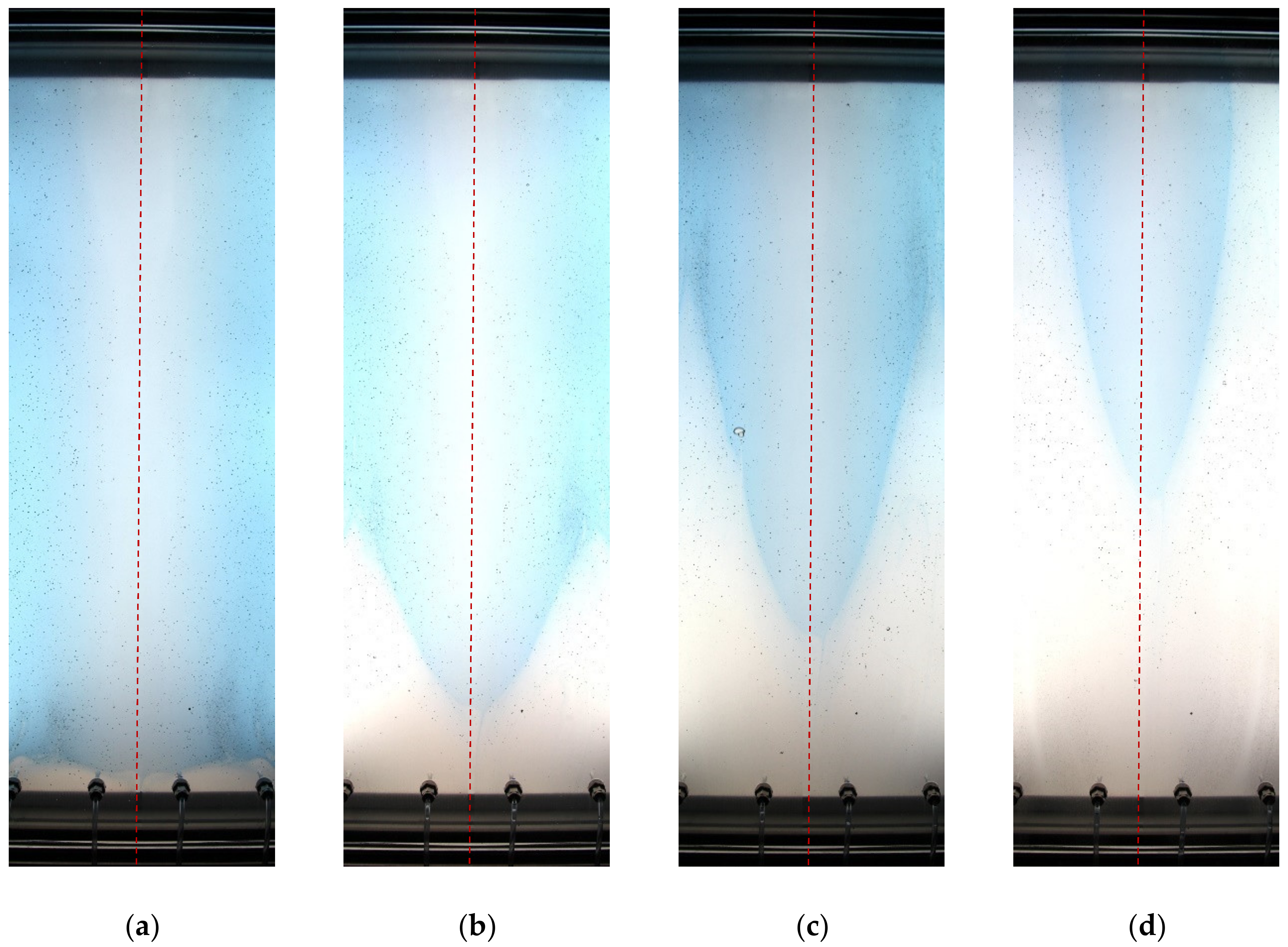
3.4. Displacement Flow Tests 6 to 9: Non-Newtonian Fluids

In tests no. 6, 7, and 8, a carbopol solution with a density of 1.00 g/cc as a displaced fluid and a carbopol and sucrose solution with a density of 1.15 g/cc as a displacing fluid are used. Figure 10 shows the rheological behavior and equivalent viscosities of these fluids. The fluids are non-Newtonian with yield-stress behavior, and yield-stress and equivalent viscosity of the displacing fluid is higher than the displaced fluid. Higher density and viscosity in the displacing fluid than the displaced fluid causes no viscous fingering in these tests. Displacement flow rates of 15.43, 21.6, and 25.53 L/min and particles with diameters of 1000 (no. 2), 3000 (no. 3), and 850 µm (no. 1) are assigned to tests no. 6, 7, and 8, respectively. For the initialization of the tests, the same procedure as before is applied, and we tried to establish a flat initial interface with very small flow rates during the initialization of the cell. Figure 11, Figure 12 and Figure 13 show snapshots of the displacement flows in these three tests, and the interfaces in these three tests at the time of zero show nearly nonflat initial interfaces. In test no. 6, a low displacement efficiency occurs compared to the previous tests due to the high equivalent viscosities of the displaced and displacing fluids. By increasing the displacement flow rates in tests 7 and 8, lower displacement efficiencies are observed due to secondary flow weakness by increasing the velocity. In test no. 8, with the highest displacement flow rate, bypassing pockets of the yield-stress displaced fluid (blue) by the displacing yield-stress fluid (white) is observed, while there is no clear evidence of this phenomena in the previous tests.
In these tests, the particles released into the displaced fluid above the interface do not have this possibility to travel downward and toward the interface and reside on it during the initialization and the main displacement flow tests because the fluids have yield-stress and the particle densities are not high enough for the downward movement of the particles. Therefore, we cannot establish a uniform spreading of the particles at the interface, as can be seen at time zero in these three tests (see Figure 11a, Figure 12a, and Figure 13a). In test no. 6 (Figure 11), after the release of particles in the cell, the particles remain in place due to yield-stress. During the initialization with a very small flow rate for adjusting the interface level on the 20 cm height, the particles move with small velocity toward the wide sides due to small secondary flow in the displaced fluid. The particle movements are discontinued when there is no flow in the cell. When the mail displacement flow starts, the particles move once again toward the wide side from the narrow side. The particles on the wide side travel with higher velocity than the interface toward the top of the cell. The particles in between the narrow and wide sides first reach the interface due to lower velocity than the interface, and when they reach the wide side due to secondary flow, their velocity increases. There are many black dots in the displaced fluid in this test because of the air bubbles. In test no. 7 (Figure 12), and similar to the previous test, the released particles remain in place after release into the cell. During the initialization, the particles on the narrow side travel upward with the same velocity as the interface, but the particles on the wide sides move up with higher velocity than the interface. This is why the distance between the particles and interface at the time zero is different in the wide and narrow sides in this test. When there is no flow in the cell, the particles remain in their place. During the main displacement flow, the particles are affected by the secondary flow in the displaced fluid and move from the narrow side toward the wide side. Simultaneously, it is observed that some particles in the wide sides move up with a higher velocity than the interface, and the ones in between the narrow and wide sides move up with a lower velocity. As shown in Figure 12b, some particles are above the interface around the wide side, and some are below the interface in between the wide and narrow sides. The ones above the interface move from the narrow side to the wide side due to secondary flow in the displaced fluid, and ones below the interface move from the wide side to the narrow side due to secondary flow in the displacing fluid. Therefore, there is a possibility for tracking the interface on the narrow side with the particles here. In test no. 8 (Figure 13), the particle behavior is similar to test no. 7. The particles released into the cell remain in place first, and during initialization, it is observed that the particles move upward toward the wide side. During the main displacement flow, the particles move from the narrow side toward the wide side, and those on the wide side travel upward with higher velocity than the interface. The particles between the narrow and wide sides first reach the interface and subsequently bypass the interface due to the lower velocity than the interface. The ones in the displaced fluid move toward the wide side, and the ones in the displacing fluid move toward the narrow side. Therefore, there is an opportunity to track the interface in the narrow side that is a more critical section during a primary cementing operation. In conclusion, we can say that top of the interface in the wide sides are tracked with all types of the used particles, and the interface on the narrow side is trackable with particles no. 3 and 1 in tests no. 7 and 8, respectively.
In test no. 9, we use another approach for tracking the interface between two fluids by using neutral buoyant particles and immersing them in the displaced or displacing fluids (displaced fluid in this case) instead of using particles with an intermediate buoyancy on the interface. The advantage of this approach is that the particles are immersed in the bulk of displaced or displacing fluids, and we know precisely which secondary flow, i.e., in the displaced or displacing fluids, is affecting the particles. The fluids used in this test are a carbopol and sucrose solution with a density of 1.027 g/cc as a displaced fluid and a carbopol and sucrose solution with a density of 1.086 g/cc as a displacing fluid. Figure 14 represents the rheological behavior and equivalent viscosities of these two fluids. Both fluids have non-Newtonian behavior with yield-stress, and the displacing fluid has higher equivalent viscosity and yield-stress than the displaced fluid. Particle no. 1 with a diameter of 850 µm and a density of 1.025 g/cc is mixed with the displaced fluid, and due to the same density of the displaced fluid and the particles, the particles are immersed in the displaced fluid. The displacement flow rate is 25.14 L/min in this test, and the same initialization approach as before is applied. Figure 15 shows the snapshots of the displacement flow in this test. It shows a poor displacement due to the high flow rate and high equivalent viscosities of the displaced and displacing fluids. By the start of the test, some particles bypass the interface due to their lower velocity than the interface. The particles above the interface are affected by the secondary flow in the displaced fluid and move slowly from the narrow side to the wide side. The bypassed particles in the displacing fluid move toward the narrow side due to the secondary flow. In real field practice with long wellbore annulus, applying this approach resulted in tracking the wide and narrow sides. This approach can be applied by immersing the particles in the displacing fluid as well. By extending the results here and in the worst-case scenario that the particles cannot overcome the secondary flow, particles immersed in the displacing fluid move toward the narrow side, and we can track the interface on the narrow side.

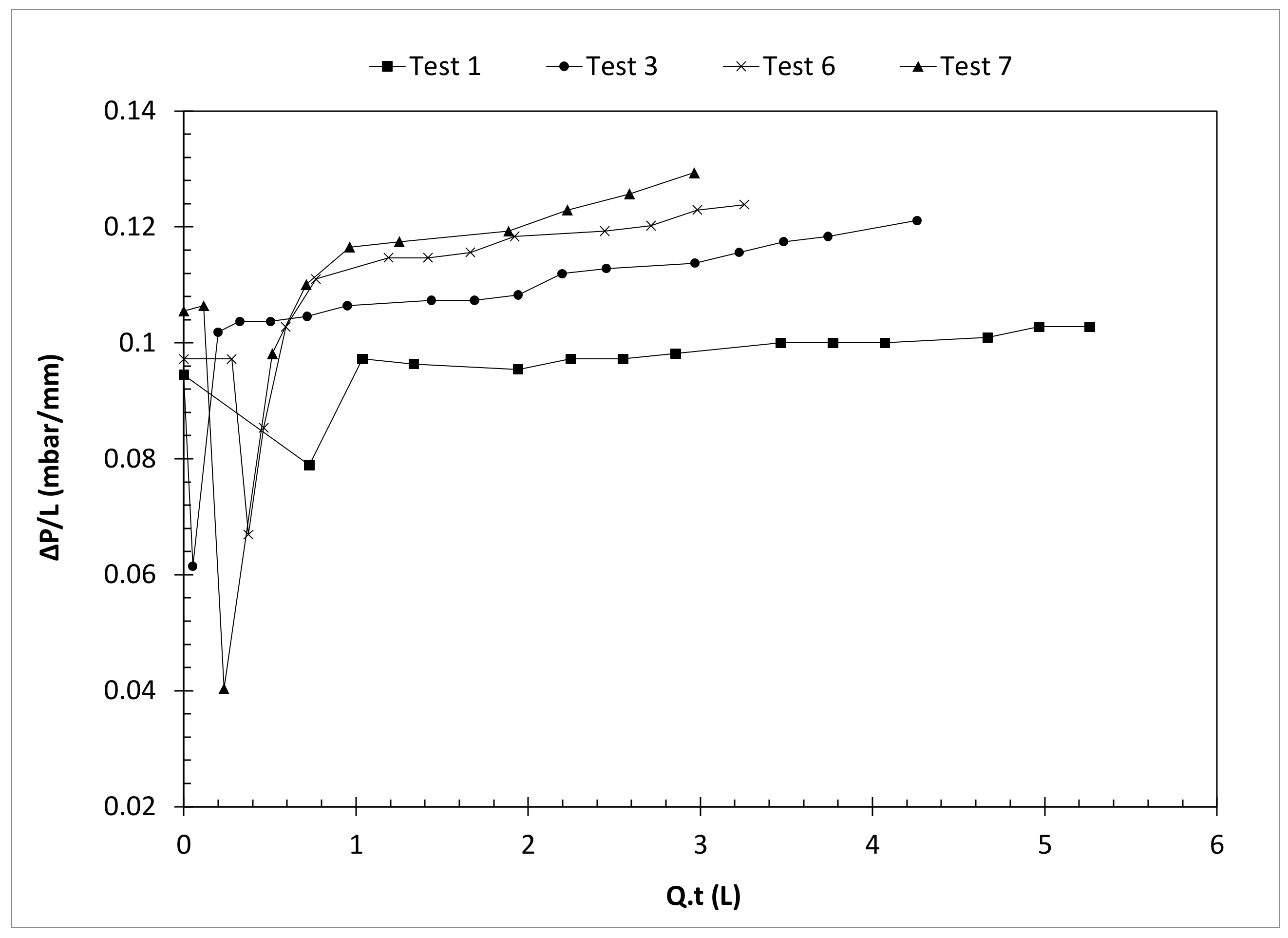
3.5. Pressure Gradient Analysis

The pressure gradients recorded by the two pressure transmitters for some of these tests in the eccentric Hele–Shaw cell were plotted in Figure 16. ΔP is the measured pressure drop involving hydrostatic and frictional pressure drops in the cell, and L is the height of the cell in these plots. The x-axis is the volume of the pumped displacing fluid from the time of zero. Over time, increasing trends are observed in the measured pressure gradients in all four tests in this graph for the displacement flow periods. Test no. 1, with two Newtonian fluids, has the lowest pressure gradient with negligible frictional pressure drop, and test no. 7, with two non-Newtonian fluids with yield-stress, has the highest pressure gradient, with a hydrostatic pressure drop similar to tests no. 1 and a considerable frictional pressure drop. Test no. 3 with a Newtonian displaced fluid, and a non-Newtonian displacing fluid is in the middle. Test no. 6 has lower pressure gradients than test no. 7 due to lower flow rate and lower frictional pressure loss. At the start of the tests, the measured pressure gradients have strange behavior because of the initial disturbances and unstable conditions due to the pumping of the fluids.
Comparison of pressure gradients of displacement flow tests in the cells with eccentric and concentric geometries [31] and with the same cross-sectional area is shown in Figure 17. Comparing the tests with the same used fluid in the concentric and eccentric geometries shows that the effect of eccentricity on the pressure gradients is not significant in these displacement flows, where the hydrostatic pressure gradient has a dominant role. In this figure, the same trends exist for displacement flow tests in these two geometries. Test no. 1 in eccentric geometry has almost the same behavior as test no. 4 in concentric geometry with the same used fluids and properties and close displacing flow rates (18.06 and 16.43 L/min in eccentric and concentric geometries). The pressure gradient in test no. 3 in eccentric geometry is comparable with test no. 5 in concentric geometry with the same used fluids (same densities and rheologies, but different effective viscosities due to different shear rates). The displacement flow rates in these two tests are far from each other; 15.27 L/min in the eccentric test and 3.71 L/min in the concentric one. The higher flow rate in eccentric geometry results in the lower effective viscosity of the displacing fluid, but their global effect on the pressure gradient is a negligible increase in pressure gradients in the eccentric geometry with the higher flow rate. By comparing test no. 7 in the eccentric geometry with test no. 7 in concentric geometries with the same used fluids, densities, and rheologies, it can be seen that the higher flow rate of 21.6 L/min in the eccentric geometry than 7.86 L/min in the concentric geometry causes lower effective viscosity, and the recorded pressure gradients in the eccentric geometry are higher than the concentric geometry. While it is known that frictional pressure drop in an eccentric annulus is lower than in a corresponding concentric annulus [24], due to the dominating hydrostatic pressure gradient and somewhat different fluid and flow properties from test to test, this is not apparent from our experiments here. The observed differences of pressure gradients in the eccentric and concentric Hele–Shaw cells are due to the flow rate differences and consequently equivalent viscosity differences rather than the degree of eccentricity.

4. Conclusions

Different displacement flow tests were performed in an eccentric Hele–Shaw cell geometry with dynamic similarity to a real field wellbore annulus during primary cementing and using different pairs of Newtonian and Herschel–Bulkley non-Newtonian fluids. The displacement efficiency, the performance of tracing particles with intermediate or neural buoyancy for tracking the interface between the displaced and displacing fluids, and the behavior of the pressure gradients in the cell were investigated. We conclude from the results that:
  • While the strong secondary flows in the tests with two Newtonian fluids cause pistonlike and highly efficient displacement, the used particles can overcome these secondary flows and track and move by the interface appropriately.
  • The relative weakness of the secondary flows in the displacement tests with a Newtonian displaced fluid and a non-Newtonian Herschel–Bulkley displacing fluid causes an almost stable and pistonlike displacement and a nonflat interface between the fluids. While 3000-µm intermediate buoyancy particles overcome these secondary flows and track the interface, smaller particle sizes (e.g., 1000-µm diameter) are affected by the secondary flows in the displacing fluid and accumulated on the narrow side. On this side, most of the particles travel toward the top with the same velocity as the interface and track it, and simultaneously some particles move toward the top with a lower velocity than the interface and bypass the interface.
  • High equivalent viscosities of the fluids in the tests with two non-Newtonian Herschel–Bulkley fluids cause very weak secondary flows, and consequently, low displacement efficiencies and nonflat interfaces between fluids. All types of the used intermediate buoyancy particles released in the displaced fluid are affected by the secondary flow and move from the narrow side toward the wide sides. The particles on the wide side travel with higher velocity than the interface toward the top and the particles between the narrow and wide sides reach the interface or bypass it due to their lower velocities than the interface. Those that reach the interface move toward the wide side due to secondary flow in the displaced fluid, and their upward velocities increase. The bypassed particles below the interface move from the wide sides to the narrow side due to secondary flow in the displacing fluid, and there will be an opportunity for tracking the interface in the narrow side that is a more critical section during a primary cementing operation.
  • Using neutral buoyant particles and immersing them in the displaced fluid in a displacement flow test shows that some of the particles bypass the interface due to their lower velocity than the interface. The particles above the interface move slowly from the narrow side to the wide sides, and the bypassed particles in the displacing fluid move toward the narrow side. In real field practice with long wellbore annulus, applying this approach resulted in tracking the wide and narrow sides. By using the neutral buoyant particles in the displacing fluid and their movement toward the narrow side in the worst scenario that the particles cannot overcome the secondary flow, we will have this hope to track the interface only on the narrow side.
  • The measured pressure gradients in the eccentric Hele–Shaw cell indicate increasing trends over time in the displacement flow tests. The tests with two Newtonian fluids have the lowest pressure gradients, and those with two non-Newtonian fluids have the highest pressure gradients, and considerable frictional pressure drops that increase by flow rate.

Author Contributions

Conceptualization, J.D.Y. and M.T.; methodology, A.T. and B.L.; validation, A.T., B.L. and J.D.Y.; formal analysis, A.T. and B.L.; investigation, A.T., B.L. and J.D.Y.; writing—original draft preparation, A.T.; writing—review and editing, A.T., B.L. and J.D.Y.; visualization, A.T.; supervision, J.D.Y. and M.T.; project administration, J.D.Y. and M.T.; funding acquisition, J.D.Y. and M.T. All authors have read and agreed to the published version of the manuscript.

Funding

This report has been produced as part of the project “Studying moving fluid interfaces during cementing of CCS wells” funded by the Research Council of Norway (268510/E20).

Institutional Review Board Statement

Not applicable.

Informed Consent Statement

Not applicable.

Data Availability Statement

No new data were created or analyzed in this study. Data sharing is not applicable to this article.

Acknowledgments

The authors would like to thank the Research Council of Norway for funding this work. The authors also thank Ali Taghipour and Martin Raphaug from SINTEF Industry for providing laboratory equipment and instrumentation. The support from Alexandre Lavrov from NTNU for designing the experiments and discussions is highly appreciated.

Conflicts of Interest

The authors declare no conflict of interest.

References

  1. Nelson, E.B.; Guillot, D. Well Cementing; Schlumberger: Houston, TX, USA, 2006. [Google Scholar]
  2. Bishop, M.; Moran, L.; Stephens, M.; Reneau, W. A robust, field friendly, cement spacer system. In Proceedings of the AADE Fluids Conference and Exhibition, Houston, TX, USA, 8–9 April 2008. AADE-08-DF-HO-07. [Google Scholar]
  3. Lavrov, A.; Torsæter, M. Physics and Mechanics of Primary Well Cementing; Springer: Berlin, Germany, 2016. [Google Scholar]
  4. Mitsuishi, N.; Aoyagi, Y. Non-newtonian fluid flow in an eccentric annulus. J. Chem. Eng. Jpn. 1973, 6, 402–408. [Google Scholar] [CrossRef] [Green Version]
  5. Jakobsen, J.; Sterri, N.; Saasen, A.; Aas, B.; Kjosnes, I.; Vigen, A. Displacements in eccentric annuli during primary cementing in deviated wells. In Proceedings of the SPE Production Operations Symposium, Oklahoma City, OK, USA, 7–9 April 1991. SPE paper no. 21686. [Google Scholar]
  6. Nouri, J.M.; Umur, H.; Whitelaw, J.H. Flow of Newtonian and non-Newtonian fluids in concentric and eccentric annuli. J. Fluid Mech. 1993, 253, 617–641. [Google Scholar] [CrossRef]
  7. Nouri, J.M.; Whitelaw, J.H. Flow of Newtonian and non-Newtonian fluids in an eccentric annulus with rotation of the inner cylinder. Int. J. Heat Fluid Flow 1997, 18, 236–246. [Google Scholar] [CrossRef]
  8. Tehrani, A.; Ferguson, J.; Bittleston, S. Laminar displacement in annuli: A combined experimental and theoretical study. In Proceedings of the SPE Annual Technical Conference and Exhibition, Washington, DC, USA, 4–7 October 1992. SPE-24569-MS. [Google Scholar]
  9. Tehrani, A.; Bittleston, S.H.; Long, P.J.G. Flow instabilities during annular displacement of one non-Newtonian fluid by another. Exp. Fluids 1993, 14, 246–256. [Google Scholar] [CrossRef]
  10. Escudier, M.P.; Gouldson, I.W.; Jones, D.M. Flow of shear-thinning fluids in a concentric annulus. Exp. Fluids 1995, 18, 225–238. [Google Scholar] [CrossRef]
  11. Escudier, M.P.; Oliveira, P.J.; Pinho, F.T.; Smith, S. Fully developed laminar low of non-Newtonian liquids through annuli: Comparison of numerical calculations with experiments. Exp. Fluids 2002, 33, 101–111. [Google Scholar] [CrossRef] [Green Version]
  12. Malekmohammadi, S.; Carrasco-Teja, M.; Storey, S.; Frigaard, I.A.; Martinez, D.M. An experimental study of laminar displacement flows in narrow vertical eccentric annuli. J. Fluid Mech. 2010, 649, 371–398. [Google Scholar] [CrossRef]
  13. Kim, Y.; Han, S.; Woo, N. Flow of Newtonian and non-Newtonian fluids in a concentric annulus with a rotating inner cylinder. Korea Aust. Rheol. J. 2013, 25, 77–85. [Google Scholar] [CrossRef]
  14. Ytrehus, J.D.; Taghipour, A.; Werner, B.; Opedal, N.; Saasen, A. Experimental study of cuttings transport efficiency of water based drilling fluids. In Proceedings of the 33rd International Conference on Ocean, Offshore and Arctic Engineering (OMAE2014), San Francisco, CA, USA, 8–13 June 2014. OMAE paper no. 2014–23960. [Google Scholar]
  15. Ytrehus, J.D.; Taghipour, A.; Sayindla, S.; Lund, B.; Werner, B.; Saasen, A. full scale flow loop experiments of hole cleaning performances of drilling fluids. In Proceedings of the 34th International Conference on Ocean, Offshore and Arctic Engineering (OMAE2015), St. John’s, NL, Canada, 31 May–5 June 2015. OMAE paper no. 2015–41901. [Google Scholar]
  16. Sayindla, S.; Lund, B.; Taghipour, A.; Werner, B.; Saasen, A.; Gyland, K.R.; Ibragimova, Z.; Ytrehus, J.D. Experimental investigation of cuttings transport with oil based drilling fluids. In Proceedings of the 35th International Conference on Ocean, Offshore and Arctic Engineering (OMAE2016), Busan, Korea, 19–24 June 2016. OMAE paper no. 2016-54047. [Google Scholar]
  17. Kettl, F.C.; Edwards, M.G.; Covington, R.L. Practical Horizontal Cementing Today. In Proceedings of the Middle East Oil Show, Manama, Bahrain, 3–6 April 1993. SPE paper no. 25546. [Google Scholar] [CrossRef]
  18. Taghavi, S.M.; Frigaard, I.A. Estimation of mixing volumes in buoyant miscible displacement flows along near-horizontal pipes. Can. J. Chem. Eng. 2013, 91, 399–412. [Google Scholar] [CrossRef]
  19. Lund, B.; Ytrehus, J.D.; Taghipour, A.; Saasen, A. Displacement Efficiency in Eccentric Annuli. In Proceedings of the 39th International Conference on Ocean, Offshore and Arctic Engineering (OMAE2020), Fort Lauderdale, FL, USA, 28 June–3 July 2020. OMAE paper no. 2020-18707. [Google Scholar]
  20. Lockyear, C.F.; Hibbert, A.P. Integrated Primary Cementing Study Defines Key Factors for Field Success. J. Pet. Technol. 1989, 41, 1320–1325. [Google Scholar] [CrossRef]
  21. Moran, L.K.; Savery, M.R. Fluid Movement Measurements Through Eccentric Annuli: Unique Results Uncovered. In Proceedings of the SPE Annual Technical Conference and Exhibition, Anaheim, CA, USA, 11–14 November 2007; p. 7. [Google Scholar]
  22. Skadsem, H.J.; Kragset, S.; Lund, B.; Ytrehus, J.D.; Taghipour, A. Annular displacement in a highly inclined irregular wellbore: Experimental and three-dimensional numerical simulations. J. Pet. Sci. Eng. 2019, 172, 998–1013. [Google Scholar] [CrossRef]
  23. Lund, B.; Ytrehus, J.D.; Taghipour, A.; Divyankar, S.; Saasen, A. Fluid-fluid displacement for primary cementing in deviated washout sections. In Proceedings of the 37th International Conference on Ocean, Offshore and Arctic Engineering (OMAE2018), Madrid, Spain, 17–22 June 2018. OMAE paper no. 2 018-78707. [Google Scholar]
  24. Lund, B.; Taghipour, A.; Ytrehus, J.D.; Saasen, A. Experimental Methods for Investigation of Drilling Fluid Displacement in Irregular Annuli. Energies 2020, 13, 5201. [Google Scholar] [CrossRef]
  25. Bittleston, S.; Ferguson, J.; Frigaard, I.A. Mud removal and cement placement during primary cementing of an oil well- Laminar non-Newtonian displacements in an eccentric annular Hele-Shaw cell. J. Eng. Math. 2002, 43, 229–253. [Google Scholar] [CrossRef]
  26. Pelipenko, S.; Frigaard, I.A. On steady state displacements in primary cementing of an oil well. J. Eng. Math. 2004, 46, 1–26. [Google Scholar] [CrossRef]
  27. Pelipenko, S.; Frigaard, I.A. Two-dimensional computational simulation of eccentric annular cementing displacements. IMA J. Appl. Math. 2004, 69, 557–583. [Google Scholar] [CrossRef]
  28. Pelipenko, S.; Frigaard, I.A. Visco-plastic fluid displacements in near-vertical narrow eccentric annuli: Prediction of travelling-wave solutions and interfacial instability. J. Fluid Mech. 2004, 520, 343–377. [Google Scholar] [CrossRef]
  29. Iyoho, A.W.; Azar, J.J. An accurate slot-flow model for non-newtonian fluid flow through eccentric annuli. Soc. Pet. Eng. J. 1981, 21, 565–572. [Google Scholar] [CrossRef]
  30. Taheri, A.; Ytrehus, J.D.; Taghipour, A.; Lund, B.; Lavrov, A.; Torsæter, M. Use of tracer particles for Tracking fluid interfaces in primary cementing. In Proceedings of the 38th International Conference on Ocean, Offshore and Arctic Engineering (OMAE2019), Glasgow, Scotland, 9–14 June 2019. OMAE paper no. 2019–96400. [Google Scholar]
  31. Taheri, A.; Ytrehus, J.D.; Lund, B.; Torsæter, M. Use of Concentric Hele-Shaw Cell for the Study of Displacement Flow and Interface Tracking in Primary Cementing. Energies 2021, 14, 51. [Google Scholar] [CrossRef]
  32. Metz, B.; Davidson, O.; de Coninck, H.C.; Loos, M.; Meyer, L.A. IPCC Special Report on Carbon Dioxide Capture and Storage; Cambridge University Press: Cambridge, UK; New York, NY, USA, 2005; 442p. [Google Scholar]
  33. Maleki, A.; Frigaard, I.A. Tracking fluid interfaces in primary cementing of surface casing. Phys. Fluids 2018, 30, 093104. [Google Scholar] [CrossRef]
  34. Frigaard, I.A.; Maleki, A. Tracking fluid interface in carbon capture and storage cement placement application. In Proceedings of the 37th International Conference on Ocean, Offshore and Arctic Engineering (OMAE2018), Madrid, Spain, 17–22 June 2018. OMAE paper no. 2018–77630. [Google Scholar]
  35. Taheri, A.; Ytrehus, J.D.; Taghipour, A.; Lund, B.; Lavrov, A.; Torsæter, M. Experimental study of the use of particles for tracking the interfaces in primary cementing of concentric and eccentric wells. In Proceedings of the SINTEF Proceedings, Trondheim, Norway, 17–19 June 2019; pp. 91–99. [Google Scholar]
  36. Qwabe, L.; Pare, B.; Jonnalagadda, S.B. Mechanism of oxidation of brilliant cresyl blue with acidic chlorite and hypochlorous acid. A kinetic approach. S. Afr. J. Chem. 2005, 58, 86–92. [Google Scholar]
Figure 1. Variation of the gap over the width in the eccentric Hele–Shaw cell.
Energies 14 01884 g001
Figure 2. Drawing of eccentric Hele–Shaw cell. (a) Top view; (b) cross-section view.
Energies 14 01884 g002
Figure 3. Experimental setup for performing the tests in the eccentric Hele–Shaw cell.
Energies 14 01884 g003
Figure 4. Snapshots of displacement flow in test no.1: (a) t = 0 s; (b) t = 5 s; (c) t = 10 s; (d) t = 15 s.
Energies 14 01884 g004
Figure 5. Snapshots of displacement flow in test no. 2: (a) t = 0 s; (b) t = 5 s; (c) t = 10 s; (d) t = 15 s.
Energies 14 01884 g005
Figure 6. Rheological behavior of the displaced and displacing fluids in tests no. 3, 4, and 5. (a) Flow curve; (b) equivalent viscosity.
Energies 14 01884 g006
Figure 7. Snapshots of displacement flow in test no. 3: (a) t = 0 s; (b) t = 6 s; (c) t = 11 s; (d) t = 17 s.
Energies 14 01884 g007
Figure 8. Snapshots of displacement flow in test no. 4: (a) t = 0 s; (b) t = 4 s; (c) t = 7 s; (d) t = 11 s.
Energies 14 01884 g008
Figure 9. Snapshots of displacement flow in test no. 5: (a) t = 0 s; (b) t = 4 s; (c) t = 8 s; (d) t = 12 s.
Energies 14 01884 g009
Figure 10. Rheological behavior of the displaced and displacing fluids in tests no. 6, 7 and 8. (a) Flow curve; (b) equivalent viscosity.
Energies 14 01884 g010
Figure 11. Snapshots of displacement flow in test no. 6. (a) t = 0 s; (b) t = 4 s; (c) t = 9 s; (d) t = 13 s.
Energies 14 01884 g011
Figure 12. Snapshots of displacement flow in test no. 7. (a) t = 0 s; (b) t = 4 s; (c) t = 9 s; (d) t = 13 s.
Energies 14 01884 g012
Figure 13. Snapshots of displacement flow in test no. 8. (a) t = 0 s; (b) t = 4 s; (c) t = 7 s; (d) t = 10 s.
Energies 14 01884 g013
Figure 14. Rheological behavior of the displaced and displacing fluids in test no. 9. (a) Flow curve; (b) equivalent viscosity.
Energies 14 01884 g014
Figure 15. Snapshots of displacement flow in test no. 9: (a) t = 0 s; (b) t = 3 s; (c) t = 5 s; (d) t = 8 s.
Energies 14 01884 g015
Figure 16. Pressure gradients in displacement flow tests in the eccentric Hele–Shaw cell.
Energies 14 01884 g016
Figure 17. Comparison of pressure gradients of displacement flow tests in the cells with eccentric and concentric geometries.
Energies 14 01884 g017
Table 1. Real and down-scaled concentric wellbore annulus data [5,8,9,12,25].
ParametersReal DataDown-Scaled Data
Length of the Cementing Section (l), m5001
Wellbore Size, in16 1/2----
Casing Size, in13 3/8----
Wellbore Radius (ro), m0.20960.05274
Casing Radius (ri), m0.16990.04275
Gap (h), m0.03970.01
Pump Rate (Q), m3/s0.023.00 × 10−4
Mean Flow Velocity ( w ¯ ), m/s0.420.10
Density of Displaced Fluid (ρ1), kg/m314401000
Density of Displacing Fluid (ρ2), kg/m318001150
Yield-Stress of Displaced Fluid (τy1), Pa4.790.2
Yield-Stress of Displacing Fluid (τy2), Pa7.050.7
Consistency Index of Displaced Fluid (κ1), Pasn0.021.59
Consistency Index of Displacing Fluid (κ2), Pasn0.034.11
Flow Behavior Index of Displaced Fluid (n1), dimensionless0.70.45
Flow Behavior Index of Displacing Fluid (n2), dimensionless10.49
Effective Shear Rate (γ.e), s−142.6140.04
Effective Viscosity of Displaced Fluid (µe1), Pas0.11890.2139
Effective Viscosity of Displacing Fluid (µe2), Pas0.19550.6434
Aspect ratio of circumferential and radial length scales (δ)0.0330.033
Aspect ratio of length and width scales (η)12598100
Reynolds Number (Re2)309.053.57
Buoyancy Number (Bu)67.252.28
Table 2. Compositions and pHs of the displaced and displacing fluids.
TestFluid TypepHCarbopol (wt/wt%)NaOH (wt/wt%)Sucrose (wt/wt%)NaCl (wt/wt%)Blue Dye (wt/wt%)
1Displaced-----0.000.00000.000000.00023
Displacing-----0.000.000350.000420.00000
2Displaced-----0.000.00000.000000.00023
Displacing-----0.000.000350.000420.00000
3Displaced-----0.000.00000.000000.00023
Displacing7.400.100.035350.000420.00000
4Displaced-----0.000.00000.000000.00023
Displacing7.400.100.035350.000420.00000
5Displaced-----0.000.00000.000000.00023
Displacing7.400.100.035350.000420.00000
6Displaced7.410.080.03200.000000.00023
Displacing6.860.100.035350.000420.00000
7Displaced7.410.080.03200.000000.00023
Displacing6.860.100.035350.000420.00000
8Displaced7.410.080.03200.000000.00023
Displacing6.860.100.035350.000420.00000
9Displaced8.080.080.03270.000000.00023
Displacing7.530.100.032210.000420.00000
Table 3. Density and rheology of the displaced and displacing fluids.
Test ρ1 (g/cc)ρ2 (g/cc)τy1 (Pa)τy2 (Pa)κ1 (Pasn)κ2 (Pasn)n1n2
111.15009.56 × 10−43.17 × 10−31.001.00
211.15009.56 × 10−43.17 × 10−31.001.00
311.1501.339.56 × 10−43.561.000.48
411.1501.339.56 × 10−43.561.000.48
511.1501.339.56 × 10−43.561.000.48
611.150.20.71.594.110.450.49
711.150.20.71.594.110.450.49
811.150.20.71.594.110.450.49
91.0271.0860.130.451.212.580.500.49
Table 4. Names and properties of the particles.
No.Particle Namedp (µm)ρp(g/cc)
1Fluorescent Green Polyethylene Microspheres710–8501.025
2Grey Polyethylene Microspheres850–10001.05
3White Polystyrene Polymer Spheres2960–30001.05
Table 5. Overview of the performed tests.
Test Displaced FluidDisplacing Fluiddp
(µm)
Q
(L/min)
γ·e
(s−1)
Re2Bu
1WaterWater + Sucrose300018.0620.09364.86924.49
2WaterWater + Sucrose100018.2820.33369.30913.36
3WaterCarbopol + Sucrose100015.2716.991.093.91
4WaterCarbopol + Sucrose300022.8625.432.053.28
5WaterCarbopol + Sucrose85022.1724.661.963.32
6CarbopolCarbopol + Sucrose100015.4317.160.983.47
7CarbopolCarbopol + Sucrose300021.624.031.642.96
8CarbopolCarbopol + Sucrose85025.5328.402.122.74
9Carbopol + SucroseCarbopol + Sucrose85025.1427.963.111.69
Publisher’s Note: MDPI stays neutral with regard to jurisdictional claims in published maps and institutional affiliations.

