Article

Collective Losses of Low Power Cage Induction Motors—A New Approach

1
Department of Electricity Power Plant, UTP University of Science and Technology in Bydgoszcz, 85-796 Bydgoszcz, Poland
2
Department of Power Electronics, Electric Machines and Drives, UTP University of Science and Technology in Bydgoszcz, 85-796 Bydgoszcz, Poland
*
Author to whom correspondence should be addressed.
Energies 2021, 14(6), 1749; https://doi.org/10.3390/en14061749
Submission received: 20 February 2021 / Revised: 15 March 2021 / Accepted: 19 March 2021 / Published: 22 March 2021

Abstract

:
Energy efficiency of systems of water pumping is a complex problem since efficiency of two distinct interacting systems needs to be combined: water and power supply. This paper introduces a non-intrusive method of calculating the so-called “collective losses” of a cage induction motor. The term “collective losses”, which the authors define, allows for accurate estimation of motor efficiency. Control system of a pump determines operating point of a pumping station, and thus its efficiency. General estimated performance characteristics of a motor, components of a control system, are assumed to serve selection of a range of pumping speed variations. Rotational speed has a direct effect on motor load torque, pump power and head, and thus on motor performance. Hellwig’s statistical method was used to specify characteristics of estimated collective losses on the basis of experimental studies of 21 motors rated at up to 2.2 kW. The results of simulations and experiments are used to verify validity and efficiency of the suggested method. The method is non-intrusive, simple to use, and requires minimum data.

1. Introduction

Analysis of energy efficiency of a water plant system is complex. Variations of plant output pressure and efficiency of pump and motor must be addressed. Energy efficiency is commonly decided by a control system applied to pump operation. In parallel, the control system is designed to provide adequate water pressure for each consumer. A pump and motor should operate in the region of maximum efficiencies, and thus of minimum losses. Minimum losses are a criterion of a control system’s operation [1]. The losses are an indication of rotational speed and motor load torque. They are directly correlated with a plant’s efficiency and output pressure. For relatively low pump capacity, rotational speed reduces relatively much, which affects the losses and motor efficiency [2].
Estimation of losses of a motor in operation (in situ) helps to develop an energy efficient control system of a pumping plant. Most traditional methods of efficiency assessment require measurements of rotor speed and shaft torque to compute output power. In most cases, torque and speed transducers cannot be installed because motors may be embedded in a machine where space is insufficient for attachment of such transducers between the motor and the load. The so-called non-intrusive motor efficiency regulator is the part of a control system that helps to improve energy efficiency without using a transducer of rotor speed and shaft torque. Therefore, indirect methods for estimating induction motor efficiency are preferable, since they do not require direct measurements of torque or speed [3,4].
The model of main losses of an induction machine (IM) consists of stator and rotor losses, mechanical losses, and core losses. Additional losses in effect of switching and conducting losses which are inside the inverter are not taken into account. Several control structures aiming to minimize losses of a squirrel-cage IM are presented in [5,6]. These methods adapt flux across a motor to operating conditions in order to attain an optimum efficiency point [7].
The Search Control (SC) is an efficiency optimization method which tracks the minimum possible input power of a motor [8,9]. This algorithm has an average delay of 15 s to arrive at the optimum operating point. In causing instability of electrical and mechanical systems, control oscillations can be obtained. This will happen, for instance, in case of pressure oscillations in the water mains.
Analysis of loss minimization control corresponds to the total loss derivative equal to zero, which produces an optimal flux [10,11]. Several applications use this technique which allows to decrease the losses, particularly in cases of lower load torques. However, since core losses are merely estimated or omitted, the value obtained at optimal flux may not be accurate.
The Maximum Torque Per Ampere (MTPA) bases on stator current curves calculated for a given IM and minimizes current in terms of torque. The MTPA method decreases motor losses. However, this method of loss minimization is not always certain to give the best results because the core losses are ignored [12,13]. The technique based on MTA approach optimizes the efficiency in scalar controlled induction motors by optimal slip control [14].
The method utilizes an improved dynamic model of IM covered in [15]. This model addresses the effect of core losses, calculated using Bertotti model, and friction mechanical parameters [16]. The proven IM model is taken to optimize scalar control and Field-Oriented Control (FOC) with decreasing total losses. FOC shows a high dynamic response and accuracy.
The Air-Gap Torque (AGT) method, based on computation of air-gap torque equations, is a commonly applied in-situ method that requires the following data to be measured: line voltages, line currents, and stator resistance [17,18]. The main strengths of this method are its accuracy and easy implementation. The no-load losses and stray losses are not considered. A no-load test is needed for calculating the friction loss and the core loss, although it should be avoided due to its intrusiveness. The Modified Induction Motor Equivalent Circuit is used for AGT method. The parameters are arrived at by solving a set of highly nonlinear and multi-dimensional equations [19].
The AGT-based method of estimating induction motor efficiency, involving online voltages, line currents, and nameplate data with a new notion of stator resistance including the Mechanical Loss Effect, was proposed in [20]. This new concept solves both the problems (stator resistance and mechanical losses estimation in AGT). The proposed objective function reduces the torque error at tFhe rated operation point, based on equations of the stator flux. However, this method does not address stray load losses. Stator resistance including the effect of mechanical losses is estimated by applying an algorithm based on Particle Swarm Optimization (PSO). This method generates good results for torque and efficiency estimation in comparison with other common methods.
Increasing the computing power of control systems allows to use artificial intelligence in estimation of motor efficiency. The genetic algorithm (GA) is one of the evolutionary algorithm methods. The estimative motor efficiency is close to the actual motor efficiency [21,22]. Another type of artificial intelligence control uses the Particle Swarm Optimization (PSO) method [23]. This model requires the motor power factor and has a relative error of 5% for 1800 RPM motors at constant speed and displays a higher uncertainty for small-sized motors or lower speed ratios. A new version of the big bang-big crunch algorithm has been proposed to estimate a three-phase motor efficiency [24]. This method is faster than PSO and GA. For estimation of motor efficiency, motor equivalent circuit is used. A comparison with other artificial intelligence methods shows that efficiency estimation is less prone to error and the results are closer to actual values.
Efficiency optimization can be realized by load observer control [25]. A motor equivalent model is used with online speed measurement. The load observer accurately estimates an unknown load disturbance. However, total motor loss consists only of stator and rotor copper loss and stator iron loss. Knowledge of parameters of the motor equivalent model is also required.
Efficiency is determined relying on equivalent circuit parameters, which are updated as a motor operates. At the same time, symmetry of these parameters is assumed for three phases of the motor [26]. In addition, power supply voltage, stator, and rotor resistances influence accuracy of efficiency calculations; what is more, this method does not cover stray load losses or mechanical losses. [27]. In effect, it is not applicable to industrial variable speed drives. An improved method of estimating parameters that serves identification of energy efficiency for an equivalent circuit is presented by [28,29]. Stray loss and friction and windage loss are derived from IEEE 112. A detailed method for determination of stray load losses is described in [30,31]. Estimation of iron losses in a motor under sinusoidal voltage supply plays an important part in the process of determining efficiency characteristics. Iron losses account for a substantial part of all the losses during frequency variations [32,33]. A new method of start-up helps to calculate motor efficiency. The test is very easy, practical, and quick to perform. It requires neither statistical nor nameplate data information. The results for the rated frequency are only described, since they are of no use to control systems [34].
The method of interpolation of total losses in induction motors in the power range 0.12–1000 kW is presented in the International Standard IEC 61800-9-2 [35]. Losses are calculated taking into account regression coefficients in terms of function of motor frequency and torque. The torque measurement for loss calculations is high intrusive. DTC or FOC electric drive control also enables torque determination. The high accuracy of the torque calculation (2%) according to the field-oriented methods makes them interesting for the determination of motor losses. The scalar control method cannot be applied. The efficiency interpolation data of typical motors two- and four-poles and efficiency class IE2 is provided.
A group of methods compute motor efficiency by means of slip measurement. They employ a linear dependence of output power on slip [36]. This method allows to estimate efficiency for rated frequency as a function of output power. High errors of efficiency estimation for other frequencies make it useless [37,38].
Another group of methods for determining efficiency of a squirrel cage motor relies on measurements of stator current [39,40]. They produce satisfactory results only for a limited range (0.7–1) of rated torque TN. Accuracy of efficiency calculation using this estimation method is not relevant.
There are many (over 30) methods for determining efficiency of a squirrel cage induction motor. A general division is based on:
  • use of motor equivalent circuit parameters,
  • study of influence of slip on motor efficiency,
  • measurement of current and voltage in stator winding,
  • measurement of rotational speed and torque,
  • analysis of no-load or load motor parameters,
  • calculation of air gap torque—AGT method,
  • efficiency optimizations techniques.
These methods generate results which estimate efficiency of induction motors only after performing additional investigations accurately or effectively. They all need no-load losses and stray losses to minimize the estimated efficiency error. This involves some intrusive steps. Table 1 shows a comparison of the methods analyzed above and what testing needs to be conducted for a given method, whether a method is highly or weakly intrusive, and what its accuracy level is.
The authors review of control systems of existing and new pump and fan drives demonstrates they often do not apply energy optimization. In order to change this situation, control systems should be modernized without substantial spending or changes to design of electric drives. A modernized control system should address the following considerations:
  • A control system should operate in-situ, that is, without additional intervention in drive design.
  • A control system should not require additional preliminary motor testing, e.g., no-load test, or inductance measurement.
  • Determination of mechanical losses and stray load losses should not require additional measurements.
  • The above assumptions are adopted for estimation of IM losses and are intended to simplify implementation procedures of control systems to new and existing electric drives with any control techniques.
In order to calculate motor efficiency, a new non-intrusive method that refers to the so-called “collective losses” is postulated. The “collective losses”, introduced by the authors, are not new losses but a group of total losses in a squirrel cage induction motor. The study is designed to determine a characteristic for their estimation as a function of frequency, voltage, and current supplied to a motor. Arguments of the estimation function are easily measurable, do not require high financial costs, and are non-intrusive. The main goal of the paper is to compare estimated and measured collective losses using the experimental model.
The newly proposed method of calculating the coefficients of explained variable, i.e., collective losses, is expressed as follows:
  • Collective losses are defined on the basis of a Sankey diagram,
  • Explaining variables necessary for a multiple regression model are determined on the basis of relative collective losses,
  • Hellwig’s method is adapted to eliminate those explaining variables that have less significant impact on the estimated collective loss function—the estimated model is simplified,
  • Coefficients, components of the predicted variable, are determined.

2. Collective Losses—Definition

Induction motor losses for in-service intervals are evaluated further on for motors of rated power below 2.2 kW. Power loss components as described by the classical theory of electric machines are shown in Figure 1. Depending on their location in a motor, the losses are classified as
Ps—stator losses, equal to Pels resulting from adverse electromagnetic effects across the stator,
Pr—rotor losses, equalling Pelr and resulting from negative electromagnetic effects across the rotor and mechanical losses Pm (bearing Pmb and windage and fan Pmf losses).
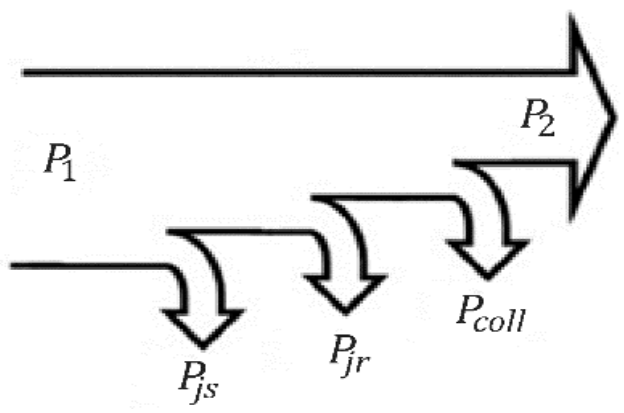
A detailed analysis of losses in a motor is highly complex and irrelevant to their in-service evaluation. The authors suggest a new, simplified distribution of power losses across a squirrel-cage induction motor to calculate output power P2. The collective losses Pcoll are introduced as a new term whose interpretation is the purpose of this paper. They comprise parts of traditional induction motor losses. Core losses Pcor, stray load losses Pstr, mechanical losses Pm, and insulation losses Pins, calculated in complicated ways, are assumed to form a single grouping, i.e., collective losses Pcoll. The remaining losses, determined by distribution of power loss components in Figure 1, are stator winding (Joule) loss Pjs and rotor winding (Joule) loss Pjr. These assumptions simplify Sankey diagram (Figure 2) [41,42,43,44]. A sinusoidal supply voltage is assumed in this discussion.
In line with the modified Sankey diagram (Figure 2), collective losses Pcoll are
P coll = P 1 P j s + P j r + P 2
The suggested method for estimation of collective losses relies on some assumptions:
a.
Accurate analysis of the individual losses is not the main goal.
b.
We assume “a priori” that an estimation characteristic of collective losses can be produced.
c.
The excess eddy-current losses are ignored. Finally, core losses Pcor consist of stator and rotor hysteresis losses Physs, Physr and stator and rotor eddy-current losses Peddys, Peddyr. Analysis of collective losses in this paper is a new approach, therefore, simplification of this method is important. If the errors are not acceptable, a new assumption is intoduced.
d.
The insulation losses Pins are omitted as they are negligible for 2.2 kW motors.
e.
Stator and rotor stray load losses Pstrs, Pstrr and stator and rotor stray no-load losses Pstr0s, Pstr0r are presented independently. This is connected with a broad range of load torque variations as defined by affinity laws for pumps and fans.
f.
The motor is supplied with a sine wave and has a variable frequency voltage source.
g.
The following relationship is realized by the voltage source: U f = const .
A component of (1), rotor Joule loss Pjr, equals slip s times electromagnetic power PΨ:
P j r = s P Ψ
The following was produced on the basis of distribution of power loss components (Figure 1):
P Ψ = P 1 P j s + P c o r s + P s t r s
The following equation is obtained on the basis of (1), (2), and (3):
P coll =   P 1 P j s n n s P 2 + s P c o r s + P s t r s
The component including slip s at (4) becomes negligible small relative to Pcoll, which ultimately become:
P coll   P 1 P j s n n s P 2
For nominal operating conditions of an induction motor, rated collective losses PcollN are defined as
P collN   P 1 N P j s N n N n s P 2 N
where
P1N—rated input power,
PjsN—rated stator Joule loss,
nN—rated rotational speed,
P2N—rated output power.
A comparison between distribution of power losses components in Figure 1 and Figure 2 shows collective losses Pcoll consist of: Pins—insulation losses, Physs, Physr—stator and rotor hysteresis losses, Peddys, Peddyr stator and rotor eddy-current losses, Pstrs, Pstrr—stator and rotor stray load losses, Pstr0s, Pstr0r—stator and rotor stray no-load losses, and Pm—mechanical losses. Pcoll are expressed by:
P coll = P i n s + P h y s s + P e d d y s + P h y s r + P e d d y r + P s t r s + P s t r r + P s t r 0 s + P s t r 0 r + P m
Equation (7) can be simplified as the following assumptions are taken into account:
  • The rotor hysteresis losses Physr are ignored because: f s f r . Such an assumption is correct for pump and fan load torque that reduces in line with the squared rotational speed in accordance with affinity laws.
  • The rotor eddy-current losses Peddyr are omitted because: f s 2 f r 2 .
  • The rotor stray load losses Pstr0r are ignored. They include rotor current Ir, which is difficult to measure. However, Ir is strongly correlated with the stator current Is.
  • Linearity of the magnetic circuit is assumed.
  • Magnetic flux densities Bzs and Bzr of the stator and rotor teeth are considered proportional to supply voltage Us and to the rotational speed n.
  • A heating power Pheat component which defines temperature increment of the motor ΔT is added, representing effect of heat on Pcoll.
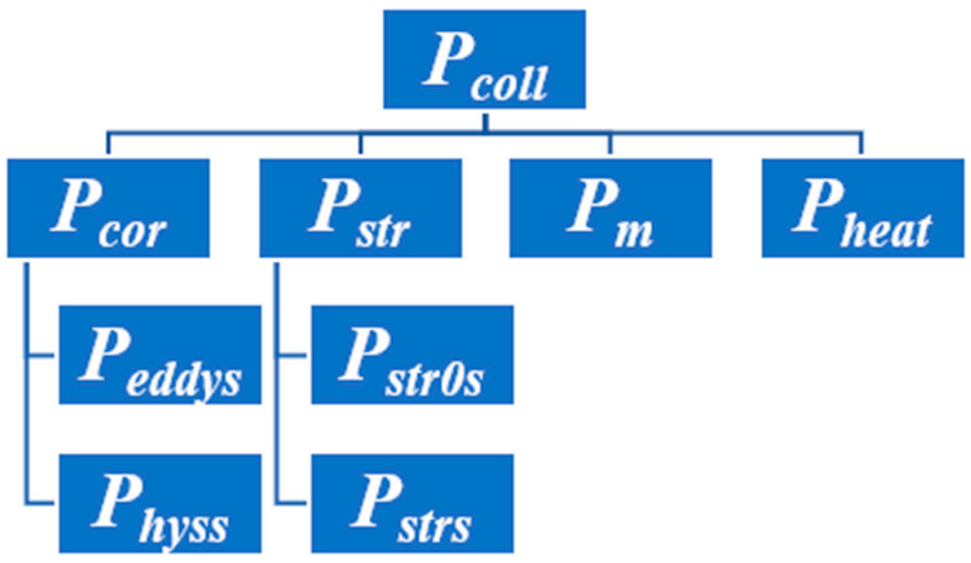
According to (7) and the above assumptions, the collective losses Pcoll can be shown in Figure 3.
and can be represented as follows:
P h y s s = c h y s s f s U s 2
P e d d y s = c e d d y s f s 2 U s 2
P s t r s = c s t r s I s 2
P s t r 0 s = c s t r 0 s B z s 2 n
P m = c m n 2
P h e a t = c τ Δ T
where chyss, ceddys, cstrs, cstr0s, cm, c𝜏—constant loss coefficients,
cτ—temperature constant.
Δ T = T f T i ; Tf—final stator winding temperature, Ti—initial stator winding temperature.
Constant loss coefficients have different values for each electric machine. The precise value of a constant helps to calculate selected loss correctly. Collective losses Pcoll represent a group of motor losses and can be estimated at an assumed accuracy. It means that other common constants can be computed for a given group of squirrel cage induction motors.
The above assumptions and set of Equation (8) are employed to convert Equation (7) into:
P coll = c h y s s f s U s 2 + c e d d y s f s 2 U s 2 + c s t r s I s 2 + c s t r 0 s U s 2 n + c m n 2 + c τ Δ T
In order to standardize the analysis and considering (9) and (6), relative collective losses P coll are defined as follows:
P coll = c 1 f s U s 2 + c 2 f s 2 U s 2 + c 3 I s 2 + c 4 U s 2 n + c 5 n 2 + c 6 Δ T
where
relative collective losses P coll are
P coll = P coll P collN
and relative constant loss coefficients c1, ..., c6 are
c 1 = c h y s s f s U s 2 P collN
c 2 = c e d d y s f s N 2 U s N 2 P collN
c 3 = c s t r s I s N P collN
c 4 = c s t r 0 s U s N 2 n N P collN
c 5 = c m n N 2 P collN
c 6 = c τ P collN

3. Test Stand

Collective losses P coll can be computed for each individual motor according to (10). It is assumed for the purposes of this paper there is a single characteristic of estimated collective loses for squirrel-cage induction motors rated below 2.2 kW. Such a characteristic can be generated on the basis of our testing of squirrel-cage induction motors. The test stand and the process of testing are described in the following part of this article.
Twenty-one squirrel-cage induction motors of both old and new motors and motors of various IE efficiency classes by six manufacturers were used in the experiments. Their rated powers ranged 0.75–2.2 kW and rated rotational speeds were 620–2900 rpm for frequency 50 Hz. Table 2 shows the rated data of some motors selected for the testing. A maximum rated power of 2.2 kW was adopted as the sole limitation. This assumption was expected to conform with testing conditions of pump energy efficiency as set out in [2]. Those authors analyzed pumps from four manufacturers with input power of up to 2.5 kW including squirrel-cage induction motors by unknown manufacturers. The sole assumption, of the maximum rated power of the motors, is reasonable.
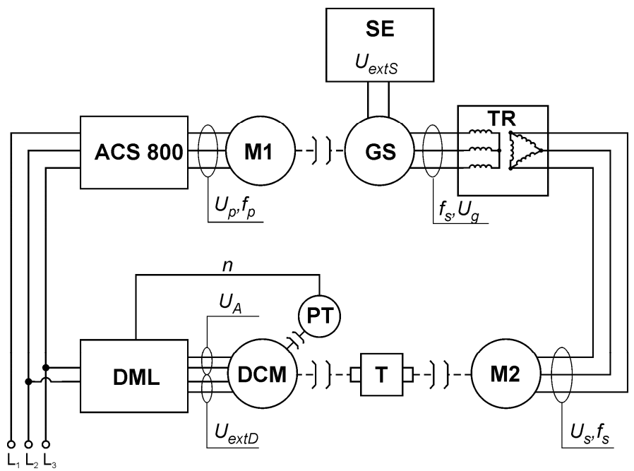
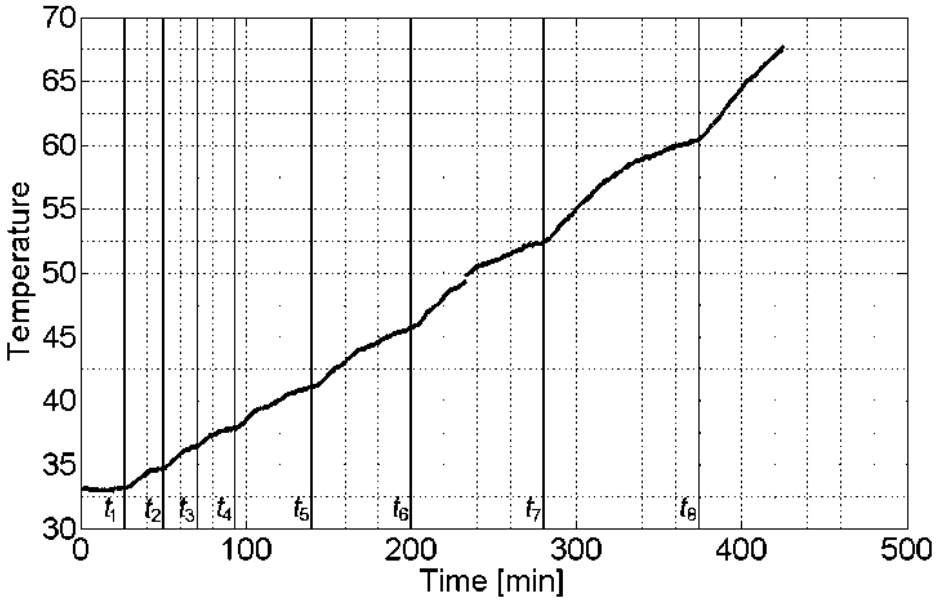
The testing was conducted in a laboratory stand shown in Figure 4. A synchronous generator GS was driven by a squirrel-cage induction motor M1 powered from a frequency converter ACS800. Change of frequency fp of Up at ACS800 output enabled variations of the M1 rotational speed and of voltage frequency fs across GS terminals. The excitation wiring was powered with voltage UextS from an SE source to arrive at a set voltage Ug. Separation Delta-Wye transformer TR was installed at the output of the synchronous generator in order to eliminate the third harmonic of Ug. Voltage Us of TR at fs was supplied to the motors tested, M2. In order to produce a desirable torque T across the shaft of M2, a DC separately excited machine DCM was coupled with M2. Winding of DCM armature was supplied with voltage UA and excitation winding was supplied with UextD from a thyristor converter DML [45]. Signal from a tachometer generator PT was provided to the DML. In effect, T across the motor shaft depended on rotational speed n of M2. A temperature sensor PT100 was mounted directly on the winding of each tested motor. To begin with, the load torque value is as desired. The motor temperature rises during the testing. In the initial time interval, close to the instant t1, the motor temperature becomes stable (temperature cannot change more than 1 °C in 1 h). This allows to measure all test values necessary to calculate collective losses. After these variable values are read, the load torque increases, then the motor temperature rises again till the next time interval close to the instant t2. With a further increase in torque, measurements are taken at subsequent instants t3, t4 and so on. An example of temperature distribution and instants t1t8 of the measurements for the supply voltage frequency of 40 Hz are illustrated in Figure 5. Every instant t1t8 corresponds to a different load torque.
The tests were performed using the following measuring devices:
  • Phase currents were measured with E3N current probes. Their accuracy was δI = 0.03. A probe signal was converted into digital signal by a 16-bit converter in a NI-USB 6361 measurement card.
  • Differential probes MTX9030-Z served to measure inter-phase voltages. The voltage measurements had a relative error of δU = 0.03 and signal damping 1/200. The probe output signal was sent to the analogue input of NI-USB 6361 16-bit measurement card.
  • Rotational speed and motor torque were measured with MT-20 and MT-10 load cells with the accuracy 0.2% of the measurement range.
  • MPS41 XX METROL mains parameter metre measured electric quantities supplied to the motor. The device analyzes the mains parameters with a satisfactory accuracy. The measurement errors are: current measurement error δI = ±0.5%, voltages measurement δU = ±0.5%, active power measurement δP = ±1%.
Over 1600 measurements were conducted for 21 tested motors. Measurement errors were below 10%. They were maximum for T lower than 50% of the rating, a consequence of measurement ranges of the metres which had been adopted.

4. Adapting Hellwig’s Method

Test results of induction motors rated PN < 2.2 kW were the starting point for one estimated characteristic of collective losses P coll . Selection of variables for econometric models was applied to this end. It was necessary to determine a computational method of finding a best-fitting subset of orthogonal linear combinations of all available predictor variables. Linear models or those that can be reduced to such models by single-equation methods are the best developed [46,47,48,49]. When there are two or more predictor variables, the model is called a “multiple regression model” with the general form:
y t = β 0 + β 1 X 1 , t + β 2 X 2 , t + , , + β k X k , t + ε t
where
y—the variable to be forecast (explained variable).
X1,…,Xkk predictor variables (explaining variable). Each of the explaining variables must be numerical.
t—time.
β1,…,βk—the coefficients measure the effect of each explaining variable after taking into account the effects of all the other explaining variables in the model.
εt—random component.
β0—constant.
The basic postulate concerning the variables’ strong correlation between each explaining and explained variable and a weak correlation between the explaining variables causes most variable selection methods to employ some versions of the linear correlation. A solution found to be optimal depends on the lowest number of mutually uncorrelated explaining variables. The explaining variables show a maximum possible correlation with the explained variable [50].
The method of optimum predicate selection, adapting Hellwig’s method [47], served to limit the number of elements of set X of originally selected explaining variables. Hellwig’s method is most popular with empirical econometric research. Its idea is to select as explaining variables such variables that are strongly correlated with an explained variable and weakly correlated with one another. Estimating a matrix R (13) of correlation coefficients between potential explaining variables and vector R (13) of correlation coefficients between potential explaining variables and vector R0 (14) of correlation coefficients between an explained variable and potential explaining variables is the starting point.
Correlation coefficients r x l x k between the particular explaining variables (Xl, Xk) form the following matrix of correlation coefficients R:
R = r x 1 x 1 r x 1 x 2 r x 1 x k r x 2 x 1 r x 2 x 2 r x 2 x k r x k x 1 r x k x 2 r x k x k K × K
Correlation coefficients r y x k between an explained variable Y and the particular explaining variables Xk form the following matrix of correlation coefficients R0:
R 0 = r y x 1 r y x 2 r y x k K × 1
The correlation coefficients r y x k and r x l x k are measured by means of Pearson’s coefficient of linear correlation r y x k between the explained variable Y and the explaining variable Xk, expressed with [49,51,52]:
r y x k = i = 1 N x i k x ¯ k y i y ¯ i = 1 N x i k x ¯ k 2 i = 1 N y i y ¯ 2
The correlation coefficient r x l x k between two explaining variables Xl and Xk is defined as
r x l x k = i = 1 N x i k x ¯ k x i l x ¯ l i = 1 N x i k x ¯ k 2 i = 1 N x i l x ¯ l 2
where N—number of measurements,
xik—ith value of the explaining variable Xk,
xil—ith value of the explaining variable Xl,
yi—ith value of the explained variable Y, and
x ¯ k —mean value of the explaining variable Xk, defined as
x ¯ k = 1 N i = 1 N x i k
y ¯ —mean value of the explained variable Y, defined as
y ¯ = 1 N i = 1 N y i
As part of Hellwig’s method, all possible combinations of potential explaining variables are generated and then the so-called integral individual ratio of information capacity is studied, produced by application of each possible combination of these variables. Selection of explaining variables for the model according to Hellwig’s method follows the procedure below.
In the first step, all possible L combinations are formed for all m explaining variables X1, ..., Xm. The number of combinations L equals the number of all possible subsets of the m-element set, that is, L = 2m − 1. For instance, if m = 2, 3 variable combinations can be produced: K1 = {X1}, K2 = {X2}, K3 = {X1, X2}.
As part of step two, for each lth combination (l = 1, ..., L), an individual ratio of information capacity hlj (19) is calculated for jth explaining variable belonging to the lth combination of variables, as formulated below:
h l j = r y x k 2 i I l | r i j |
where
I l = i : X i K l —set of variable indices as part of lth combination Kl;
hlj—individual capacity of jth variable in lth combination Kl;
r y x k —correlation coefficient of kth explaining variable with the endogenous (explained) variable y;
i = I l r i j —total sum of absolute correlation coefficients of jth explaining variable with the remaining explaining variables included in the combination Kl.
The third step involves calculation of individual capacity of potential explaining variables (Hl) as the total sum of individual capacities as part of each combination, as formulated below:
H l = j = I l h l j , l = 1 , , L
Explaining variables X belonging to that subset of lth combination to which a maximum value of Hl corresponds are selected to the multiple regression model (12), i.e.,
H l = max l 1 , , L H l

5. Statistical Model of Collective Losses P coll

The prediction of relative collective losses P coll (10) is performed in this chapter. The linear multiple regression model in line with (12) was accepted for the purposes of analysis. Explaining variables Xk (where k∈{1,2…m}) are expressed with the quantities, parts of vector X, which are tested in the real model as a function of time [2]:
X = X 1 X 2 X 3 X 4 X 5 X 6 = f s U s 2 f s 2 U s 2 I s 2 U s 2 n n 2 Δ T
Coefficients β1,…,βk (12) correspond to the constants c1, ..., c6 from (10); the definition is offered:
Y = C X + c 0
where vector C consists of relative constant loss coefficients c1, ..., c6:
C =   c 1 , c 2 , c 3 , c 4 , c 5 , c 6
Finally, the predicted variable Y as a linear multiple regression model is defined as
Y = c 0 + c 1 X 1 + c 2 X 2 + c 3 X 3 + c 4 X 4 + c 5 X 5 + c 6 X 6
The linear multiple regression model required optimization of the number of explaining variables and determination of coefficients c0...c6. To this end, we measured the following electric and mechanical quantities as part of our experimentation: torque, rotational speed, voltages, currents, motor winding temperature, and frequency. About 1600 test samples were produced for 21 motors. Using the measurement data, the vector X explaining variables (22) was generated on the basis of (10) that defines relative collective losses and the multiple regression model (12).
Explaining variables Xk for the predicted variable Y was selected according to the following formal and statistical criteria:
  • the explaining variables Xk in the predicted variable Y should have coefficients of correlation νk > 0.2—the method of eliminating quasi-constant variables,
  • the coefficients of correlation between the explaining variables Xk, and the explained variable Y should tend towards one,
  • the coefficients of correlation between the explaining variables Xk should tend towards one zero,
  • the degree of matching of the predicted variable Y to results of real measurements should be maximum possible, which is expressed as maximization of the determination coefficient R2.
The analyses showed the above criteria are met for all the explaining variables Xk.
Hellwig’s method was applied to the next stage of selection of the explaining variables Xk. Based on the correlation coefficients r y x k (15) and r x l x k (16), Hellwig’s ratio of integral capacity Hl is analyzed for all combinations of l without repeating the explaining variables remaining in the model. L = 2m − 1 of the combinations for m = 6 explaining variables equals 63. The individual ratio of information capacity for ith combination, Kl, is calculated as per (19).
Out of all the combinations of explaining variables Xk one l is selected for which Hellwig’s ratio of integral capacity becomes maximum Hlmax = max (Hl) (21). Following Hellwig’s method, the number of explaining variables Xk is reduced. Two explaining variables, X1 and X3, remain in the model of relative collective losses for which the explained variable Ye is defined as follows:
Y e = c e 0 + c e 1 X 1 + c e 2 X 3
where
ce0, ce1, ce2—coefficients of explained variable Ye of relative collective losses P coll .
The simplified model of the predicted variable Y was subject to statistical verification to check if the selected variables X1 and X3 have significant impact on the explained variable Y and whether the criteria of applicability of the least-squares method to determination of the coefficients c0, c1, c3 of the model are fulfilled. The model’s statistical verification proceeded by:
  • Testing significance of the model’s coefficients with Student’s t-test.
  • Testing of the model’s matching to empirical data:
    • calculation of the determination coefficient,
    • calculation of the convergence coefficient,
    • calculation of the random variability coefficient.
  • Verification of the random structure’s properties:
    • testing randomness of a random component with the runs test,
    • testing normalcy of a random component’s distribution,
    • testing homogeneity of a random component’s variance with White’s test.
The analyses demonstrated the selected variables X1 and X3 have significant impact on the explained variable Ye. Finally, the explained variable Ye (26) depends on two variables, X1 and X3, and is described with three coefficients: c0, c1 and c3. The mean square approximation, also named the minimum chi-square method, where a minimum sum Δmin is sought, served to compute these coefficients [48,49]:
Δ min = i = 1 N y m i y e i 2
where
i—number of a measurement,
ymi—measured value of relative collective losses,
yei—value of predicted variable, estimated by the model (26) for the ith measurement.
The minimum chi-square method reaches function factors by means of matrix calculus. The method can be applied if the following assumptions are met:
a.
The model is linear or can be reduced to a linear form,
b.
A linear dependence holds between no interpretative variables,
c.
The number of measurements serving to estimate factors exceeds the number of factors estimated in this manner,
d.
The expected value of a random component equals zero E(ε) = 0.
In order to estimate the model coefficients (ce0, ce1, ce2), a coefficient vector Ce is arrived at according to [51,52]:
C e = M T · M 1 · M T · Y m
where
Ym—vector of measured values ymi of relative collective losses, defined as
Y m = y m 1 y m 2 y m N
Ce—vector of the model coefficients is given as
C e = c e 0 c e 1 c e 2
M—observation matrix of the explaining variables is defined as
M = 1 X 11 X 31 1 X 12 X 32 1 X 1 N X 3 N
ce0, ce1, ce2, computed as per (28), were substituted to (26) and values of the predicted variable Y were calculated as
Y e = 4.7 + 45 X 1 + 23 X 3 10 3
The predicted variable Ye considering (10) enables to define the model for estimation of relative collective losses P coll :
P coll = 4.7 + 45 f s U s 2 + 23 I s 2 10 3
Relative estimation collective losses P coll (33) were compared to measured experimental values.

6. Simulation and Testing Analyses

Variations of estimated relative collective losses P ecoll were analyzed on the basis of calculation results as per (33). Based on (5) and (6), variations of tested relative collective losses P tcoll expressed as follows could be analyzed:
P t coll P 1 P j s n n s P 2 P 1 N P j s N n N n s P 2 N
Calculations of estimated P ecoll (33) and tested P tcoll (34) relative collective losses required measurement of the following quantities: f—frequency of supply voltage, Us—supply voltage to induction motor, Is—stator current, R—resistance of stator winding, n—rotational speed, P1—input power, TL—torque across motor shaft, T—temperature of stator winding. Temperature is not directly present in the model of relative collective losses, nevertheless, it affects winding resistance.
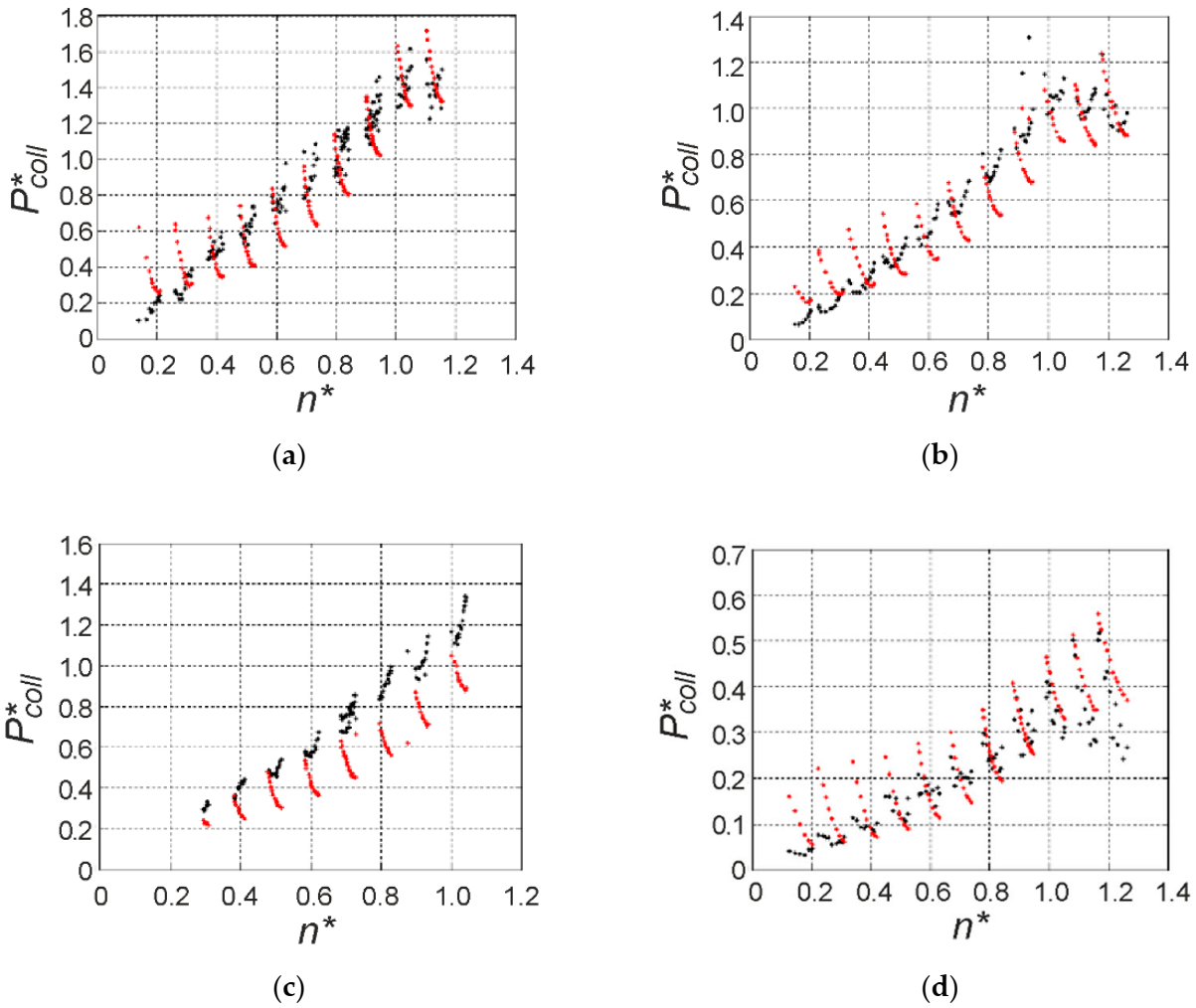
To compare estimated P ecoll and tested P tcoll collective losses, losses of 21 motors operating at different rotational speeds and loads were tested. Rotational speed was in the range (0.2–1) nN. For selected motors, maximum rotational speed reached 1.2nN. A thyristor converter DML and a separately excited machine DCM helped to maintain a constant load torque TL for the tested motor M2 during a single test. The load torque ranged (0.1–1.1) TLN (TLN—rated load torque). The real range of load torque variations TL depended on the frequency of voltage supplied to M2. For lower frequencies, maximum load torque reduces if the motor current is below the rated value IN. The calculation results are shown in Figure 6. Tested P tcoll collective losses are represented with black dots, while estimated P ecoll collective losses are represented with red dots. The results form sets of dots around selected values of rotational speed n*. For instance, the set of dots around the relative rotational speed n* = 1 determines values of relative collective losses P tcoll and P ecoll for f = 50 Hz selected values of load torque TL in the range (0.1–1.1) TN. As f declines, corresponding to lower rotational speeds n*, maximum load torque reduces. The resultant black and red dot sets for a selected frequency largely overlap in Figure 6a,b,d. The results illustrated in Figure 6c are evidence of relatively high divergences.
The coefficient of determination R2 is an indication of how correct the results are. R2 for the entire test group of 21 motors is calculated as 80%. This means the selection of explaining variables is good. Higher values of R2 represent quality of matching of an estimated model to a real motor. R2 values for individual motors range 70–97%. This means the selection of explaining variables for estimation of collective loss characteristic curve P ecoll is satisfactory, good, or very good. Examples of R2 are presented in Table 2. The results can be seen as satisfactory. They reaffirm the prior assumption an estimated characteristic of collective losses exists in a squirrel cage induction motor is correct.
The statistical group encompasses 21 new and in-service motors by different manufacturers. This ensures universality of the results. The suggested approach is non-intrusive and can be used by industry to control on-line motor losses. To estimate collective losses, only measured values of frequency, supply voltage, and motor current must be taken into consideration. The instrumentation in this method is cost-effective, which justifies its particular applicability to low power pump drives.
The results suggest a need for further testing of 2.2–7.5 kW motors. They are part of many electric drives of pump systems. Existence of an estimated characteristic for collective losses shows motor efficiency needs to be verified. Such an estimated efficiency would be especially useful in control of water pump stations in order to improve energy efficiency.

7. Conclusions

In this paper, a non-intrusive method of estimating the so called “collective losses” of squirrel-cage induction motors of rated power 0.75–2.2 kW has been utilized. The term “collective losses” has been introduced. In order to determine coefficients of a collective loss curve, Hellwig’s information capacity method has been used. The results have demonstrated the method’s accuracy, with a good agreement between measured and estimated collective losses in an induction motor fed with a sinusoidal voltage source in the range of 10–60 Hz.
Determination of estimated collective losses is non-intrusive. It is necessary only to measure (33) frequency, voltage, and current of an induction motor. Additionally, temperature of the motor windings should be monitored. A comparison of this method of collective loss calculation with known techniques of motor loss calculation leads to the following conclusions:
In the new method of collective loss calculation:
  • No load test is required.
  • IEEE 112 standard or other test methods are not used to determine stray load losses,
  • A torque metre does not need to be mounted on the motor shaft—the method is non-intrusive.
  • Any control system of electric drive can be used—V/f, DTC, FOC, VVC, or others,
  • The estimated characteristic of the collective losses includes a minimum of explaining variables—Hellwig’s optimization.
  • The estimated characteristic of the collective losses addresses both new motors and motors after years of service.
  • The estimated characteristic of the collective losses addresses motors of various efficiency classes.
  • Collective losses are computed for broad ranges of frequency (10–60) Hz and torque (0.1–1.1) TN variations.
  • Collective loss calculation requires only measurement of supply voltage, motor current, and frequency.
These results are part of our research oriented towards improvement of pumping efficiency of water or sewage. If a satisfactory convergence is confirmed between estimated and measured characteristics of motor efficiency, the efficiency of an entire pumping unit can be controlled. Practical application of this solution to PLCs will improve energy effectiveness of new and in-service water and sewage pumping stations.

Author Contributions

Conceptualization, E.S. and L.S.; methodology, L.S. and E.S.; software, L.S.; validation, E.S.; formal analysis, L.S.; investigation, L.S.; resources, E.S.; data curation, L.S.; writing—original draft preparation, L.S.; visualization, L.S.; supervision, L.S.; project administration, E.S. All authors have read and agreed to the published version of the manuscript.

Funding

This research received no external funding.

Institutional Review Board Statement

Not applicable.

Informed Consent Statement

Not applicable.

Data Availability Statement

There is no report of any data.

Conflicts of Interest

The authors declare no conflict of interest.

Nomenclature

ffrequency (Hz)
fNrated frequency (Hz)
Iscurrent of stator winding (A)
INrated current (A)
nrotational speed (rpm)
Ppower (kW)
PNrated power (kW)
Usvoltage across stator winding (V)
P1input motor power (kW)
P2output motor power (kW)
PΨelectromagnetic power (kW)
Pjsstator Joule loss (kW)
Pjrrotor Joule loss (kW)
Pcollcollective losses (kW)
PcollNrated collective losses (kW)
Pcorrrotor core losses (kW)
Pcorsstator core losses (kW)
Pstrrrotor stray load losses (kW)
Pstrsstator stray load losses (kW)
Pstr0stray no-load losses (kW)
Pmmechanical losses (kW)
Pinsinsulation losses (kW)
sslip
TNrated motor torque (Nm)
TLload torque (Nm)
TLNrated load torque (Nm)
Usvoltage across stator winding (V)
ηmotor efficiency
P coll = P coll P collN relative collective losses
f s = f s f N relative frequency of motor supply voltage
n = n n N relative rotational speed
I s = I s I N relative current of stator winding
U s = U s U N relative voltage across stator winding
T = T L T L N relative load torque

References

  1. Bidstrup, N.; Hunnekuhl, G.; Heinrich, H.; Andersen, T. Classification of Circulators; Europump: Brussels, Belgium, 2003. [Google Scholar]
  2. Szychta, L.; Figura, R. Analysis of efficiency characteristics of squirrel-cage induction motor for pump applications. In Proceedings of the 2012 XXth International Conference on Electrical Machines, Marseille, France, 2–5 September 2012; Institute of Electrical and Electronics Engineers (IEEE): Piscataway, NJ, USA, 2012; pp. 73–78. [Google Scholar]
  3. Salomon, C.P.; Sant’Ana, W.C.; Lambert-Torres, G.; Da Silva, L.E.B.; Bonaldi, E.L.; Oliveira, L.E.D.L.D.; Da Silva, L.B. Comparison among Methods for Induction Motor Low-Intrusive Efficiency Evaluation Including a New AGT Approach with a Modified Stator Resistance. Energies 2018, 11, 691. [Google Scholar] [CrossRef] [Green Version]
  4. Parasiliti, F.; Bertoldi, P. Energy Efficiency in Motor Driven Systems; Springer: Berlin/Heidelberg, Germany, 2003. [Google Scholar]
  5. Razali, R. Improving squirrel cage induction motor efficiency: Technical review. Int. J. Phys. Sci. 2012, 7, 1129–1140. [Google Scholar] [CrossRef]
  6. Agamloh, E.B. A Comparison of direct and indirect measurement of induction motor efficiency. In Proceedings of the 2009 IEEE International Electric Machines and Drives Conference, Miami, FL, USA, 3–6 May 2009; Institute of Electrical and Electronics Engineers (IEEE): Piscataway, NJ, USA, 2009; pp. 36–42. [Google Scholar]
  7. Hsu, J.; Kueck, J.; Olszewski, M.; Casada, D.; Otaduy, P.; Tolbert, L. Comparison of induction motor field efficiency evaluation methods. IEEE Trans. Ind. Appl. 1998, 34, 117–125. [Google Scholar] [CrossRef] [Green Version]
  8. Cleland, J.; McCormick, V.; Turner, M. Design of an efficiency optimization controller for inverter-fed AC induction motors. In Proceedings of the IAS ’95. Conference Record of the 1995 IEEE Industry Applications Conference Thirtieth IAS Annual Meeting, Orlando, FL, USA, 8–12 October 1995; Institute of Electrical and Electronics Engineers (IEEE): Piscataway, NJ, USA, 2002; Volume 1, pp. 16–21. [Google Scholar]
  9. Kirschen, D.S.; Novotny, D.W.; Lipo, T.A. On-Line Efficiency Optimization of a Variable Frequency Induction Motor Drive. IEEE Trans. Ind. Appl. 1985, IA-21, 610–616. [Google Scholar] [CrossRef]
  10. Qu, Z.; Ranta, M.; Hinkkanen, M.; Luomi, J. Loss-Minimizing Flux Level Control of Induction Motor Drives. IEEE Trans. Ind. Appl. 2012, 48, 952–961. [Google Scholar] [CrossRef] [Green Version]
  11. Waheedabeevi, M.; Sukeshkumar, A.; Nair, N.S. New online loss- minimization-based control of scalar and vector-controlled induction motor drives. In Proceedings of the 2012 IEEE International Conference on Power Electronics, Drives and Energy Systems (PEDES), Bengaluru, India, 16–19 December 2012; Institute of Electrical and Electronics Engineers (IEEE): Piscataway, NJ, USA, 2012; pp. 1–7. [Google Scholar]
  12. Bojoi, R.; Li, Z.; Odhano, S.A.; Griva, G.; Tenconi, A.; Bojoi, I.R. Unified direct-flux vector control of induction motor drives with maximum torque per ampere operation. IEEE Energy Convers. Congr. Expo. 2013, 3888–3895. [Google Scholar] [CrossRef]
  13. Wasynczuk, O.; Sudhoff, S.; Corzine, K.; Tichenor, J.; Krause, P.; Hansen, I.; Taylor, L. A maximum torque per ampere control strategy for induction motor drives. IEEE Trans. Energy Convers. 1998, 13, 163–169. [Google Scholar] [CrossRef] [Green Version]
  14. Cacciato, M.; Consoli, A.; Scarcella, G.; Scelba, G.; Testa, A. Efficiency optimization techniques via constant optimal slip control of induction motor drives. In Proceedings of the International Symposium on Power Electronics, Electrical Drives, Automation and Motion, Taormina, Italy, 23–26 May 2006; Institute of Electrical and Electronics Engineers (IEEE): Piscataway, NJ, USA, 2006; pp. 33–38. [Google Scholar]
  15. Khoury, M.G. Energy Efficiency Improvement of a Squirrel-Cage Induction Motor through the Control Strategy. Ph.D. Thesis, Institut Polytechnique de Toulouse, Toulouse, France, 2018. [Google Scholar]
  16. Bertotti, G. General properties of power losses in soft ferromagnetic materials. IEEE Trans. Magn. 1988, 24, 621–630. [Google Scholar] [CrossRef]
  17. Figura, R. Nonintrusive Method of Estimating Efficiency of Squirrel-Cage Induction Motor. Ph.D. Thesis, Technical University of Radom, Radom, Poland, 2012. [Google Scholar]
  18. Lu, B.; Habetler, T.G.; Harley, R.G. A Nonintrusive and In-Service Motor-Efficiency Estimation Method Using Air-Gap Torque with Considerations of Condition Monitoring. IEEE Trans. Ind. Appl. 2008, 44, 1666–1674. [Google Scholar] [CrossRef]
  19. Lu, B.; Habetler, T.G.; Harley, R.G. A Nonintrusive Efficiency Estimation Method for In-Service Motor Testing using a Modified Induction Motor Equivalent Circuit. In Proceedings of the 37th IEEE Power Electronics Specialists Conference, Jeju, Korea, 18–22 June 2006; Institute of Electrical and Electronics Engineers (IEEE): Piscataway, NJ, USA, 2006; pp. 1–6. [Google Scholar]
  20. Da Silva, L.E.B.; Cortez, A.D.; Salomon, C.P.; Santana, W.C.; Lambert-Torres, G.; Bonaldi, E.L.; Oliveira, L.E.D.L.D.; Da Silva, J.G.B. Differential Evolution based Air-Gap Torque method approach for induction motor efficiency estimation. In Proceedings of the 2015 18th International Conference on Intelligent System Application to Power Systems (ISAP), Porto, Portugal, 11–16 September 2015; Institute of Electrical and Electronics Engineers (IEEE): Piscataway, NJ, USA, 2015; pp. 1–6. [Google Scholar]
  21. Karnavas, Y.; Vacharides, C.; Karlis, A. On the development of an on-site induction motor efficiency estimator framework. MedPower 2014, 73–76. [Google Scholar] [CrossRef]
  22. Pillay, P.; Levin, V.; Otaduy, P.; Kueck, J. In-situ induction motor efficiency determination using the genetic algorithm. IEEE Trans. Energy Convers. 1998, 13, 326–333. [Google Scholar] [CrossRef]
  23. Li, Y.; Liu, M.; Lau, J.; Zhang, B. A novel method to determine the motor efficiency under variable speed operations and partial load conditions. Appl. Energy 2015, 144, 234–240. [Google Scholar] [CrossRef]
  24. Bigdeli, M.; Azizian, D.; Rahimpour, E. An Improved Big Bang-Big Crunch Algorithm for Estimating Three-Phase Induction Motors Efficiency. J. Oper. Autom. Power Eng. 2016, 4, 83–92. [Google Scholar]
  25. Chen, C.; Yu, H.; Gong, F.; Wu, H. Induction Motor Adaptive Backstepping Control and Efficiency Optimization Based on Load Observer. Energies 2020, 13, 3712. [Google Scholar] [CrossRef]
  26. Guru, B.S.; Hiziroglu, H.R. Electric Machinery and Transformers, 3rd ed.; Oxford University Press: Oxford, UK, 2001. [Google Scholar]
  27. Stermecki, A.; Biro, O.; Preis, K.; Rainer, S.; Krischan, K.; Ofner, G. Calculation of load-dependent equivalent circuit parameters of squirrel cage induction motors using time-harmonic FEM. In Proceedings of the 18th International Conference on Electrical Machines, Vilamoura, Portugal, 6–9 September 2008; Institute of Electrical and Electronics Engineers (IEEE): Piscataway, NJ, USA, 2008; Volume 29, pp. 1–6. [Google Scholar]
  28. Aminu, M.; Barendse, P.; Khan, A. A Simplified Equivalent Circuit Method for Induction Machine Nonintrusive Field Efficiency Estimation. IEEE Trans. Ind. Electron. 2019, 67, 7301–7311. [Google Scholar] [CrossRef]
  29. Wang, G.; Park, S.-W. Improved Estimation of Induction Motor Circuit Parameters with Published Motor Performance Data. In Proceedings of the 2014 Sixth Annual IEEE Green Technologies Conference, Corpus Christi, TX, USA, 3–4 April 2014; Institute of Electrical and Electronics Engineers (IEEE): Piscataway, NJ, USA, 2014; pp. 25–28. [Google Scholar]
  30. Boglietti, A.; Cavagnino, A.; Ionel, D.M.; Popescu, M.; Staton, D.A.; Vaschetto, S. A General Model to Predict the Iron Losses in PWM Inverter-Fed Induction Motors. IEEE Trans. Ind. Appl. 2010, 46, 1882–1890. [Google Scholar] [CrossRef]
  31. Boglietti, A.; Bojoi, R.; Cavagnino, A.; Vaschetto, S.; Bojoi, I.R. Influence of the sinusoidal supply frequency on the induction motor stray load losses. In Proceedings of the IECON 2012—38th Annual Conference on IEEE Industrial Electronics Society, Montreal, QC, Canada, 25–28 October 2012; Institute of Electrical and Electronics Engineers (IEEE): Piscataway, NJ, USA, 2012; pp. 1847–1851. [Google Scholar]
  32. Boglietti, A.; Cavagnino, A.; Lazzari, M. Fast Method for the Iron Loss Prediction in Inverter-Fed Induction Motors. IEEE Trans. Ind. Appl. 2010, 46, 806–811. [Google Scholar] [CrossRef] [Green Version]
  33. Wang, K.; Huai, R.; Yu, Z.; Zhang, X.; Li, F.; Zhang, L. Comparison Study of Induction Motor Models Considering Iron Loss for Electric Drives. Energies 2019, 12, 503. [Google Scholar] [CrossRef] [Green Version]
  34. Rengifo, J.; Albanez, E.; Benzaquen, J.; Bueno, A.; Aller, J.M. Full-Load Range In-Situ Efficiency Estimation Method for Induction Motors Using Only A Direct Start-Up. In Proceedings of the 2018 XIII International Conference on Electrical Machines (ICEM), Alexandroupoli, Greece, 3–6 September 2018; Institute of Electrical and Electronics Engineers (IEEE): Piscataway, NJ, USA, 2018; pp. 1213–1219. [Google Scholar]
  35. British Standard. Adjustable Speed Electrical Power Drive Systems Part 9-2: Ecodesign for Power Drive Systems, Motor Starters, Power Electron-ICS and Their Driven Applications—Energy Efficiency Indicators for Power Drive Systems and Motor Starters; IEC61800-9-2; British Standard: London, UK, 2017. [Google Scholar]
  36. Kueck, J.D. Assessment of Methods for Estimating Motor Efficiency and Load under Field Conditions; ORNL/TM-13165; Oak Ridge National Laboratory: Oak Ridge, TN, USA, 1996.
  37. Kueck, J.D.; Gray, J.R.; Driver, R.C.; Hsu, J. Assessment of Available Methods for Evaluating in Service Motor Efficiency; Oak Ridge National Laboratory: Oak Ridge, TN, USA, 1996. [Google Scholar]
  38. Ontario Hydro. In-Plant Electric Motor Loading and Efficiency Techniques; TSDD-90-043; Ontario Hydro: Toronto, ON, Canada, 1990. [Google Scholar]
  39. Tiainen, R.; Sarkimaki, V.; Ahola, J.; Lindh, T.; Niemelä, M. Current measurement-based detection of load torque changes in a variable speed VSI induction motor drive to support motor diagnostics. In Proceedings of the 2007 European Conference on Power Electronics and Applications, Aalborg, Denmark, 2–5 September 2007; Institute of Electrical and Electronics Engineers (IEEE): Piscataway, NJ, USA, 2007; pp. 1–10. [Google Scholar]
  40. McCoy, G.A.; Douglas, J.G. Energy Management for Motor Driven System; U.S. DOE: Washington, DC, USA, 2000.
  41. Chapman, S.J. Electric Machinery Fundamentals; McGraw Hill: New York, NY, USA, 2012. [Google Scholar]
  42. Krause, P.C. Analysis of Electric Machinery; McGraw Hill: Singapore, 1986. [Google Scholar]
  43. Jordan, H.E. Energy Efficient Electric Motors and their Applications; VAN Nostrand Reinhold, Co.: New York, NY, USA, 1983. [Google Scholar]
  44. Gieras, J.F. Electrical Machines—Fundamentals at Electromechanical Energy Conversion; CRC Press: Boca Raton, FL, USA, 2016. [Google Scholar]
  45. Szychta, L.; Figura, R.; Kwiecień, R. Application of a Thyristor Drive Assembly DML to Testing of Mechanical Characteristics of Asynchronous Motors, 12TH International Conference Computer Systems Aided Science, Industry and Transport; TransComp: Zakopane, Poland, 1–4 December 2008. [Google Scholar]
  46. Hyndman, R.J.; Athanasopoulos, G. Forecasting: Principles and Practice; OText: Melbourne, Australia, 2018. [Google Scholar]
  47. Hellwig, Z. Linear Regression and Its Applications to Economics; Pergamon Press: Oxford, UK, 1963. [Google Scholar]
  48. Miller, A. Subset Selection in Regression; CRC Press: Boca Raton, FL, USA, 2002. [Google Scholar]
  49. Osinska, M. Ekonometria Współczesna; Dom Organizatora: Toruń, Poland, 2007. [Google Scholar]
  50. Sowinski, J. The Impact of the Selection of Exogenous Variables in the ANFIS Model on the Results of the Daily Load Forecast in the Power Company. Energies 2021, 14, 345. [Google Scholar] [CrossRef]
  51. Borkowski, B.; Dudek, H.; Szczęsny, W. Econometrics. Selected Problems; PWN: Warsaw, Poland, 2003. [Google Scholar]
  52. Nowak, E. An Outline of Econometric Methods; PWN: Warsaw, Poland, 1998. [Google Scholar]
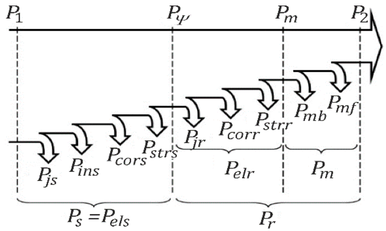
Figure 1. Distribution of power loss components: P1—input power, P2—output power, Ps—stator losses, Pr—rotor losses, Pm—mechanical losses, Pmb—bearings losses, Pmf—windage and fan losses, PΨ—electromagnetic power, Pjs—stator Joule loss, Pjr—rotor Joule loss, Pins—insulation losses, Pcors, Pcorr—stator and rotor core losses, Pstrs, Pstrr—stator and rotor stray load losses.
Energies 14 01749 g001
Figure 2. A simplified Sankey diagram: P1—input power, P2—output power, Pcoll—collective losses, Pjs—stator winding (Joule) loss, Pjr—rotor winding (Joule) loss.
Energies 14 01749 g002
Figure 3. A block diagram showing parts of collective losses Pcoll, Pcor—core losses, Physs—stator hysteresis losses, Peddys stator eddy-current losses, Pstrs—stator stray load losses, Pstr0s—stator stray no-load losses, Pm—mechanical losses, Pheat—heating power.
Energies 14 01749 g003
Figure 4. A laboratory stand for testing induction motors M2.
Energies 14 01749 g004
Figure 5. Temperature chart for the frequency 40 Hz and eight different values of the load torque.
Energies 14 01749 g005
Figure 6. Tested (black) P t coll and estimated (red) collective losses P ecoll as a function of rotational speed n* for: (a) motor 1, (b) motor 2, (c) motor 3, (d) motor 4 (Table 2).
Energies 14 01749 g006
Table 1. Comparison of methods of motor efficiency determination.
MethodNo Load TestStray Load LossRotational Speed or Torque DeterminationHigh IntrusiveLow IntrusiveNo-IntrusiveEfficiency Calculation Accuracy
Measurement of rotational speedNoNoYesYes--High
Slip methodNoNoYesYes--Low
Equivalent circuit diagramYesIEEE 112No-Yes-Low
Current and voltage measurementNoNoNo--YesLow
AGTYesIEEE 112No-Yes-High
No load current methodYesNoNo-Yes-Low
Artificial intelligenceYesIEEE 112No-Yes-High
Load observerYesIEEE 112No-Yes-High
Optimizations techniquesYesNoYes-Yes-High
Table 2. The rated data of selected motors.
NoPNUNINnNcosφηNR2
12.24004.814250.80.820.97
21.53803.714200.80.770.95
32.2400528700.770.830.97
41.14002.714150.80.740.8
51.54004.29000.820.630.89
60.754001.8813950.80.720.7
71.13802.628700.840.770.7
81.54003.228350.830.820.7
Publisher’s Note: MDPI stays neutral with regard to jurisdictional claims in published maps and institutional affiliations.