
Examining the Linkages among Carbon Dioxide Emissions, Electricity Production and Economic Growth in Different Income Levels


Abstract
1. Introduction
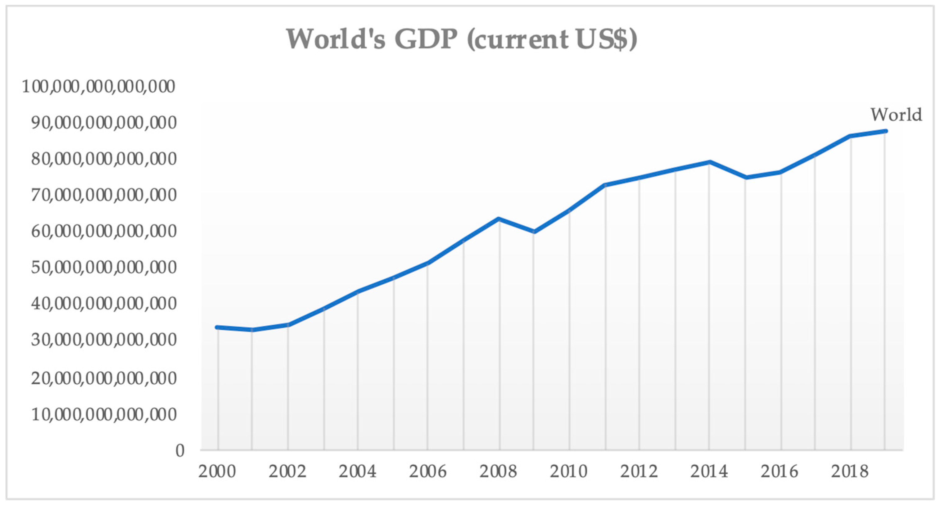
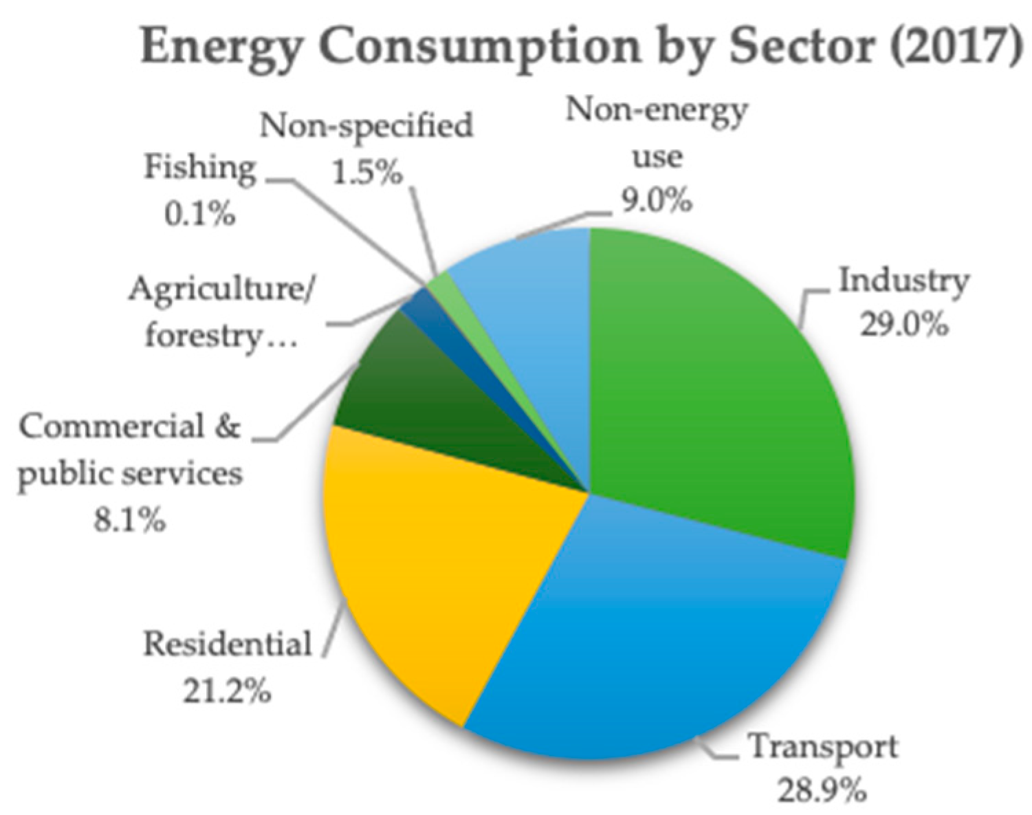
2. Recent World Data
3. Literature Review
4. Materials and Methods
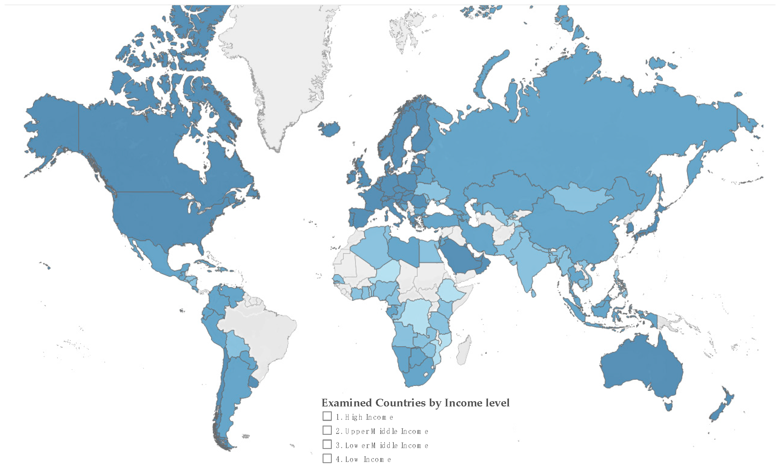
4.1. Data
4.2. Econometric Methodology
5. Results
5.1. Descriptive Statistical Analysis
5.2. Cross-Section Dependence and Unit Roots
5.3. Cointegration
5.4. Regression Results
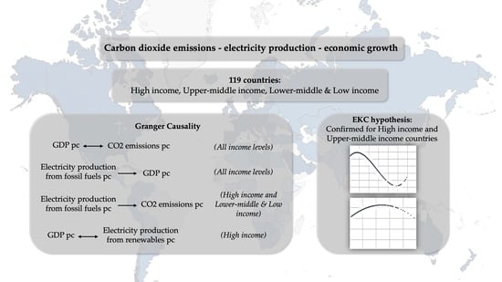
5.5. Granger Causality
6. Discussion
7. Conclusions and Policy Implications
Author Contributions
Funding
Institutional Review Board Statement
Informed Consent Statement
Data Availability Statement
Conflicts of Interest
References
- Höök, M.; Tang, X. Depletion of fossil fuels and anthropogenic climate change—A review. Energy Policy 2013, 52, 797–809. [Google Scholar] [CrossRef]
- Chiari, L.; Zecca, A. Constraints of fossil fuels depletion on global warming projections. Energy Policy 2011, 39, 5026–5034. [Google Scholar] [CrossRef]
- EPA. Greenhouse Gas. Emissions. United States Environmental Protection Agency. Available online: https://www.epa.gov/ghgemissions/overview-greenhouse-gases (accessed on 23 December 2020).
- Masnadi, M.S.; Grace, J.R.; Bi, X.T.; Lim, C.J.; Ellis, N. From fossil fuels towards renewables: Inhibitory and catalytic effects on carbon thermochemical conversion during co-gasification of biomass with fossil fuels. Appl. Energy 2015, 140, 196–209. [Google Scholar] [CrossRef]
- EIA. International Energy Outlook 2019; US Energy Information Administration: Washington, DC, USA, 2019.
- World Bank. CO2 Emissions (kt). The World Bank Data. Available online: https://data.worldbank.org/indicator/EN.ATM.CO2E.KT (accessed on 23 December 2020).
- World Bank. Energy Use (kg of Oil Equivalent per Capita). The World Bank Data. Available online: https://data.worldbank.org/indicator/EG.USE.PCAP.KG.OE (accessed on 23 December 2020).
- Levitan, O.; Dinamarca, J.; Hochman, G.; Falkowski, P.G. Diatoms: A fossil fuel of the future. Trends Biotechnol. 2014, 32, 117–124. [Google Scholar] [CrossRef]
- Lotfalipour, M.R.; Falahi, M.A.; Ashena, M. Economic growth, CO2 emissions, and fossil fuels consumption in Iran. Energy 2010, 35, 5115–5120. [Google Scholar] [CrossRef]
- Adams, S.; Klobodu, E.K.M.; Apio, A. Renewable and non-renewable energy, regime type and economic growth. Renew. Energy 2018, 125, 755–767. [Google Scholar] [CrossRef]
- Bölük, G.; Mert, M. Fossil & renewable energy consumption, GHGs (greenhouse gases) and economic growth: Evidence from a panel of EU (European Union) countries. Energy 2014, 74, 439–446. [Google Scholar]
- World Bank. GDP (Current US$). The World Bank Data. Available online: https://data.worldbank.org/indicator/NY.GDP.MKTP.CD (accessed on 23 December 2020).
- World Bank. Population, Total. The World Bank Data. Available online: https://data.worldbank.org/indicator/SP.POP.TOTL (accessed on 23 December 2020).
- World Bank. GDP Per Capita (Current US$). The World Bank Data. Available online: https://data.worldbank.org/indicator/NY.GDP.PCAP.CD (accessed on 11 September 2020).
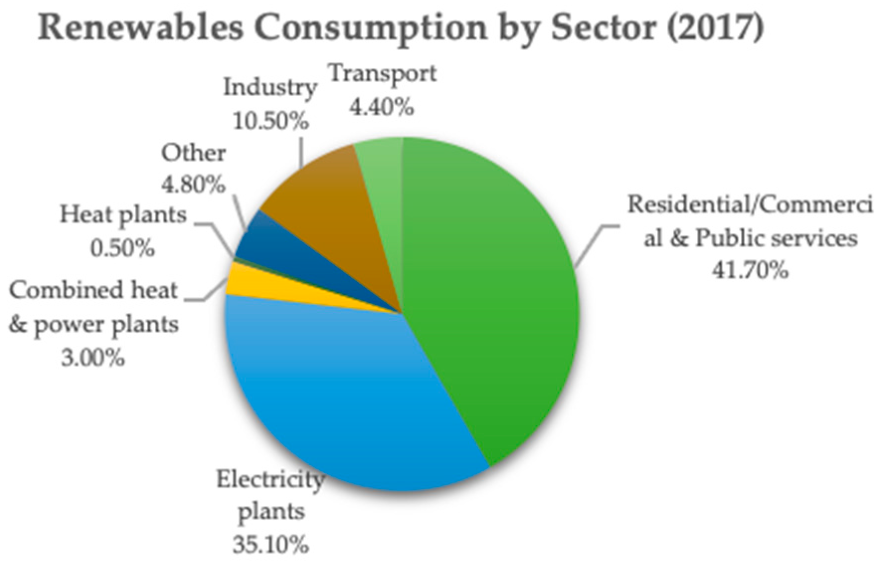
- IEA. Total Final Consumption (TFC) by Sector, World 1990–2017. Data and Statistics. Available online: https://www.iea.org (accessed on 23 December 2020).
- IEA. Renewable Share in Final Energy Consumption (SDG 7.2), World 1990–2017. Data and Statistics. Available online: https://www.iea.org (accessed on 23 December 2020).
- IEA. Total CO2 Emissions, World 1990–2017. Data and Statistics. Available online: https://www.iea.org (accessed on 23 December 2020).
- IEA. CO2 Emissions per Capita, World 1990–2017. Data and Statistics. Available online: https://www.iea.org (accessed on 23 December 2020).
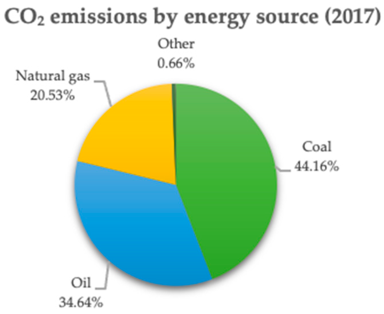
- IEA. CO2 Emissions by Energy Source, World 1990–2017. Data and Statistics. Available online: https://www.iea.org (accessed on 23 December 2020).
- World Bank. Forest Area (sq. km). The World Bank Data. Available online: https://data.worldbank.org/indicator/AG.LND.FRST.K2 (accessed on 23 December 2020).
- Dinda, S. Environmental Kuznets Curve Hypothesis: A Survey. Ecol. Econ. 2004, 49, 431–455. [Google Scholar] [CrossRef]
- Adamu, T.M.; Haq, I.U.; Shafiq, M. Analyzing the Impact of Energy, Export Variety, and FDI on Environmental Degradation in the Context of Environmental Kuznets Curve Hypothesis: A Case Study of India. Energies 2019, 12, 1076. [Google Scholar] [CrossRef]
- Beşer, M.K.; Beşer, B.H. The Relationship between Energy Consumption, CO2 Emissions and GDP per Capita: A Revisit of the Evidence from Turkey. Alphanumer. J. 2017, 5, 353–368. [Google Scholar] [CrossRef]
- Bongers, A. The Environmental Kuznets Curve and the Energy Mix: A Structural Estimation. Energies 2020, 13, 2641. [Google Scholar] [CrossRef]
- Shahbaz, M.; Khraief, N.; Uddin, G.S.; Ozturk, I. Environmental Kuznets curve in an open economy: A bounds testing and causality analysis for Tunisia. Renew. Sustain. Energy Rev. 2014, 34, 325–336. [Google Scholar] [CrossRef]
- Apergis, N.; Ozturk, I. Testing Environmental Kuznets Curve hypothesis in Asian countries. Ecol. Indic. 2015, 52, 16–22. [Google Scholar] [CrossRef]
- Jebli, M.B.; Youssef, S.B.; Ozturk, I. Testing environmental Kuznets curve hypothesis: The role of renewable and non-renewable energy consumption and trade in OECD countries. Ecol. Indic. 2016, 60, 824–831. [Google Scholar] [CrossRef]
- Li, T.; Wang, Y.; Zhao, D. Environmental Kuznets Curve in China: New evidence from dynamic panel analysis. Energy Policy 2016, 91, 138–147. [Google Scholar] [CrossRef]
- Kang, Y.-Q.; Zhao, T.; Yang, Y.-Y. Environmental Kuznets curve for CO 2 emissions in China: A spatial panel data approach. Ecol. Indic. 2016, 63, 231–239. [Google Scholar] [CrossRef]
- Dong, K.; Sun, R.; Hochman, G. Do natural gas and renewable energy consumption lead to less CO2 emission? Empirical evidence from a panel of BRICS countries. Energy 2017, 141, 1466–1478. [Google Scholar] [CrossRef]
- Al-Mulali, U.; Saboori, B.; Ozturk, I. Investigating the environmental Kuznets curve hypothesis in Vietnam. Energy Policy 2015, 76, 123–131. [Google Scholar] [CrossRef]
- Ozturk, I.; Al-Mulali, U. Investigating the validity of the environmental Kuznets curve hypothesis in Cambodia. Ecol. Indic. 2015, 57, 324–330. [Google Scholar] [CrossRef]
- Abdallh, A.A.; Abugamos, H. A semi-parametric panel data analysis on the urbanization—Carbon emissions nexus for the MENA countries. Renew. Sustain. Energy Rev. 2017, 78, 1350–1356. [Google Scholar] [CrossRef]
- Özokcu, S.; Özdemir, Ö. Economic growth, energy, and environmental Kuznets curve. Renew. Sustain. Energy Rev. 2017, 72, 639–647. [Google Scholar] [CrossRef]
- Mehrara, M. Energy consumption and economic growth: The case of oil exporting countries. Energy Policy 2007, 35, 2939–2945. [Google Scholar] [CrossRef]
- Narayan, P.K.; Smyth, R. Energy consumption and real GDP in G7 countries: New evidence from panel cointegration with structural breaks. Energy Econ. 2008, 30, 2331–2341. [Google Scholar] [CrossRef]
- Apergis, N.; Payne, J.E. Renewable energy consumption and economic growth: Evidence from a panel of OECD countries. Energy Policy 2010, 38, 656–660. [Google Scholar] [CrossRef]
- Ozturk, I.; Aslan, A.; Kalyoncu, H. Energy consumption and economic growth relationship: Evidence from panel data for low and middle income countries. Energy Policy 2010, 38, 4422–4428. [Google Scholar] [CrossRef]
- Apergis, N.; Payne, J.E. The renewable energy consumption—Growth nexus in Central America. Appl. Energy 2011, 88, 343–347. [Google Scholar] [CrossRef]
- Wang, S.; Zhou, D.; Zhou, P.; Wang, Q. CO2 emissions, energy consumption and economic growth in China: A panel data analysis. Energy Policy 2011, 39, 4870–4875. [Google Scholar] [CrossRef]
- Lu, W.-C. Renewable energy, carbon emissions, and economic growth in 24 Asian countries: Evidence from panel cointegration analysis. Environ. Sci. Pollut. Res. 2017, 24, 26006–26015. [Google Scholar] [CrossRef]
- Lin, B.; Moubarak, M. Renewable energy consumption—Economic growth nexus for China. Renew. Sustain. Energy Rev. 2014, 40, 111–117. [Google Scholar] [CrossRef]
- Pao, H.-T.; Tsai, C.-M. Modeling and forecasting the CO2 emissions, energy consumption, and economic growth in Brazil. Energy 2011, 36, 2450–2458. [Google Scholar] [CrossRef]
- Pao, H.-T.; Yu, H.-C.; Yang, Y.-H. Modeling the CO2 emissions, energy use, and economic growth in Russia. Energy 2011, 36, 5094–5100. [Google Scholar] [CrossRef]
- Soytas, U.; Sari, R.; Ewing, B.T. Energy consumption, income, and carbon emissions in the United States. Ecol. Econ. 2007, 62, 482–489. [Google Scholar] [CrossRef]
- Acaravci, A.; Ozturk, I. On the relationship between energy consumption, CO2 emissions and economic growth in Europe. Energy 2010, 35, 5412–5420. [Google Scholar] [CrossRef]
- Pirlogea, C.; Cicea, C. Econometric perspective of the energy consumption and economic growth relation in European Union. Renew. Sustain. Energy Rev. 2012, 16, 5718–5726. [Google Scholar] [CrossRef]
- Kasman, A.; Duman, Y.S. CO2 emissions, economic growth, energy consumption, trade and urbanization in new EU member and candidate countries: A panel data analysis. Econ. Model. 2015, 44, 97–103. [Google Scholar] [CrossRef]
- Alper, A.; Oguz, O. The role of renewable energy consumption in economic growth: Evidence from asymmetric causality. Renew. Sustain. Energy Rev. 2016, 60, 953–959. [Google Scholar] [CrossRef]
- Pablo-Romero, M.D.P.; Sánchez-Braza, A. Residential energy environmental Kuznets curve in the EU–28. Energy 2017, 125, 44–54. [Google Scholar] [CrossRef]
- Hundie, S.K.; Daksa, M.D. Does energy-environmental Kuznets curve hold for Ethiopia? The relationship between energy intensity and economic growth. J. Econ. Struct. 2019, 8, 21. [Google Scholar] [CrossRef]
- Aruga, K. Investigating the Energy-Environmental Kuznets Curve Hypothesis for the Asia-Pacific Region. Sustain. J. Rec. 2019, 11, 2395. [Google Scholar] [CrossRef]
- Luzzati, T.; Orsini, M. Investigating the energy-environmental Kuznets curve. Energy 2009, 34, 291–300. [Google Scholar] [CrossRef]
- Abdou, D.M.S.; Atya, E.M. Investigating the energy-environmental Kuznets curve: Evidence from Egypt. Int. J. Green Econ. 2013, 7, 103. [Google Scholar] [CrossRef]
- Pablo-Romero, M.D.P.; De Jesús, J. Economic growth and energy consumption: The energy-environmental Kuznets curve for Latin America and the Caribbean. Renew. Sustain. Energy Rev. 2016, 60, 1343–1350. [Google Scholar] [CrossRef]
- Asumadu-Sarkodie, S.; Owusu, P.A. The relationship between carbon dioxide emissions, electricity production and consumption in Ghana. Energy Sources Econ. Plan. Policy 2017, 24, 1–12. [Google Scholar] [CrossRef]
- Mohiuddin, O.; Asumadu-Sarkodie, S.; Obaidullah, M. The relationship between carbon dioxide emissions, energy consumption, and GDP: A recent evidence from Pakistan. Cogent Eng. 2016, 3, 1210491. [Google Scholar] [CrossRef]
- Bento, J.P.C.; Moutinho, V. CO2 emissions, non-renewable and renewable electricity production, economic growth, and international trade in Italy. Renew. Sustain. Energy Rev. 2016, 55, 142–155. [Google Scholar] [CrossRef]
- Al-Mulali, U.; Weng-Wai, C.; Sheau-Ting, L.; Mohammed, A.H. Investigating the environmental Kuznets curve (EKC) hypothesis by utilizing the ecological footprint as an indicator of environmental degradation. Ecol. Indic. 2015, 48, 315–323. [Google Scholar] [CrossRef]
- Ulucak, R.; Bilgili, F. A reinvestigation of EKC model by ecological footprint measurement for high, middle and low income countries. J. Clean. Prod. 2018, 188, 144–157. [Google Scholar] [CrossRef]
- Serajuddin, U.; Hamadeh, N. New World Bank Country Classifications by Income Level: 2020–2021. World Bank Blogs. Available online: https://blogs.worldbank.org/opendata/new-world-bank-country-classifications-income-level-2020-2021# (accessed on 11 February 2021).
- IEA. Total Production. Electricity. Data and Statistics. Available online: https://www.iea.org (accessed on 11 February 2021).
- World Bank. Electricity Production from Oil, Gas and Coal Sources (% of Total). The World Bank Data. Available online: https://data.worldbank.org/indicator/EG.ELC.FOSL.ZS (accessed on 11 February 2021).
- World Bank. Electricity Production from Renewable Sources, Excluding Hydroelectric (% of Total). The World Bank Data. Available online: https://data.worldbank.org/indicator/EG.ELC.RNWX.ZS (accessed on 11 February 2021).
- World Bank. Electricity Production from Hydroelectric Sources (% of Total). The World Bank Data. Available online: https://data.worldbank.org/indicator/EG.ELC.HYRO.ZS (accessed on 11 February 2021).
- World Bank. CO2 Emissions (Metric Tons per Capita). The World Bank Data. Available online: https://data.worldbank.org/indicator/EN.ATM.CO2E.PC (accessed on 11 February 2021).
- World Bank. Population Density (People per sq. km of Land Area). The World Bank Data. Available online: https://data.worldbank.org/indicator/EN.POP.DNST (accessed on 11 February 2021).
- Halkos, G.E. Environmental Kuznets Curve for sulfur: Evidence using GMM estimation and random coefficient panel data models. Environ. Dev. Econ. 2003, 8, 581–601. [Google Scholar] [CrossRef]
- Halkos, G.; Petrou, K.N. The relationship between MSW and education: WKC evidence from 25 OECD countries. Waste Manag. 2020, 114, 240–252. [Google Scholar] [CrossRef]
- Pedroni, P. Fully Modified OLS for Heterogeneous Cointegrated Panels. In Nonstationary Panels, Panel Cointegration, and Dynamic Panels (Advances in Econometrics); Elsevier: Amsterdam, The Netherlands, 2004; pp. 93–130. [Google Scholar]
- Revathy, A.; Paramasivam, P. Study on Panel Co-integration, Regression and Causality Analysis in Papaya Markets of India. Int. J. Curr. Microbiol. Appl. Sci. 2018, 7, 40–49. [Google Scholar] [CrossRef]
- Hall, A.R. Generalized Method of Moments; Oxford University Press: Oxford, UK, 2005. [Google Scholar]
- Hall, A.R. Generalized Method of Moments. In Handbook of Research Methods and Applications in Empirical Macroeconomics; Edward Elgar Publishing: Cheltenham, UK, 2013. [Google Scholar]
- Yin, G. Bayesian generalized method of moments. Bayesian Anal. 2009, 4, 191–207. [Google Scholar] [CrossRef]
- Ahmad, M.; Khan, R.E.A. Does Demographic Transition with Human Capital Dynamics Matter for Economic Growth? A Dynamic Panel Data Approach to GMM. Soc. Indic. Res. 2018, 142, 753–772. [Google Scholar] [CrossRef]
- Ullah, S.; Akhtar, P.; Zaefarian, G. Dealing with endogeneity bias: The generalized method of moments (GMM) for panel data. Ind. Mark. Manag. 2018, 71, 69–78. [Google Scholar] [CrossRef]
- Liu, Y.; Hao, Y. The dynamic links between CO2 emissions, energy consumption and economic development in the countries along “the Belt and Road”. Sci. Total Environ. 2018, 645, 674–683. [Google Scholar] [CrossRef] [PubMed]
- Harris, R.; Sollis, R. Applied Time Series Modelling and Forecasting; Wiley: Hoboken, NJ, USA, 2003. [Google Scholar]
- Arellano, M.M.; Bond, S. Dynamic Panel Data Estimation Using DPD—A Guide for Users; Working Paper Series; Institute for Fiscal Studies: London, UK, 1988. [Google Scholar]
- Mocking, R.; Steegmans, J. Capital Structure Determinants and Adjustment Speed: An Empirical Analysis of Dutch SMEs; No. 357. rdf; CPB Netherlands Bureau for Economic Policy Analysis: Hague, The Netherlands, 2017. [Google Scholar]
- Ribeiro, H.V.; Rybski, D.; Kropp, J.P. Effects of changing population or density on urban carbon dioxide emissions. Nat. Commun. 2019, 10, 1–9. [Google Scholar] [CrossRef]
- Gudipudi, R.; Fluschnik, T.; Ros, A.G.C.; Walther, C.; Kropp, J.P. City density and CO2 efficiency. Energy Policy 2016, 91, 352–361. [Google Scholar] [CrossRef]
- Markard, J. The next phase of the energy transition and its implications for research and policy. Nat. Energy 2018, 3, 628–633. [Google Scholar] [CrossRef]
- Sareen, S.; Haarstad, H. Bridging socio-technical and justice aspects of sustainable energy transitions. Appl. Energy 2018, 228, 624–632. [Google Scholar] [CrossRef]
- Sustainable Development Goals—SDGs—The United Nations. The 17 Goals. Available online: https://sdgs.un.org/goals (accessed on 20 January 2020).


| Income Level | Threshold (July 2020) |
|---|---|
| High income | >12,535 |
| Upper-middle income | 4046–12,535 |
| Lower-middle income | 1036–4045 |
| Low income | <1036 |
| Source | Indicator | Measurement | |
|---|---|---|---|
| 1 | IEA [62] | Total electricity production | GWh |
| 2 | WB [13] | Population | total |
| 3 | WB [63] | Electricity production from oil, gas and coal sources | % of total |
| 4 | WB [64] | Electricity production from renewable sources, excluding hydroelectric | % of total |
| 5 | WB [65] | Electricity production from hydroelectric sources | % of total |
| 6 | WB [66] | CO2 emissions | Metric tons per capita |
| 7 | WB [14] | GDP per capita | Current US$ |
| 8 | WB [67] | Population density | People per sq. km of land area |
| EPFpc | EPRpc | CO2pc | GDPpc | Dens | |
|---|---|---|---|---|---|
| Mean | 0.004684 | 0.003144 | 10.39119 | 32,195.14 | 336.1680 |
| Median | 0.003691 | 0.000939 | 8.072146 | 27,729.19 | 109.5809 |
| Maximum | 0.021955 | 0.056814 | 67.31050 | 118,823.6 | 7952.998 |
| Minimum | 0.00000331 | 0 | 0.251345 | 1659.908 | 2.493134 |
| Std. Dev. | 0.004552 | 0.007736 | 8.274268 | 21,106.53 | 1028.928 |
| Skewness | 1.748568 | 4.755374 | 2.960003 | 1.164747 | 5.988748 |
| Kurtosis | 5.968018 | 28.28739 | 15.53083 | 4.738511 | 39.83826 |
| Jarque-Bera | 782.8296 | 27158.6 | 7146.537 | 314.3716 | 55,831.77 |
| Prob. | 0.0000 | 0.0000 | 0.0000 | 0.0000 | 0.0000 |
| EPFpc | EPRpc | CO2pc | GDPpc | Dens | |
|---|---|---|---|---|---|
| Mean | 0.001757 | 0.000913 | 4.215383 | 5545.145 | 72.05436 |
| Median | 0.001421 | 0.000494 | 3.306489 | 4986.676 | 65.22279 |
| Maximum | 0.005999 | 0.010049 | 15.6463 | 19288.6 | 270.9931 |
| Minimum | 0 | 0 | 0.657959 | 622.7421 | 2.179756 |
| Std. Dev. | 0.001496 | 0.001577 | 3.090284 | 3226.249 | 58.80999 |
| Skewness | 0.751483 | 4.073107 | 1.262113 | 1.008053 | 1.092193 |
| Kurtosis | 2.593474 | 20.94012 | 4.227859 | 4.117945 | 4.357204 |
| Jarque-Bera | 63.3315 | 10141.95 | 205.8481 | 138.8408 | 172.7788 |
| Prob. | 0.0000 | 0.0000 | 0.0000 | 0.0000 | 0.0000 |
| EPFpc | EPRpc | CO2pc | GDPpc | Dens | |
|---|---|---|---|---|---|
| Mean | 0.000432 | 0.000232 | 1.139077 | 1470.063 | 134.9511 |
| Median | 0.000188 | 0.000133 | 0.611946 | 1133.186 | 73.57522 |
| Maximum | 0.002133 | 0.002499 | 15.1386 | 5591.212 | 1239.579 |
| Minimum | 0 | 0 | 0.01628 | 111.9272 | 1.543177 |
| Std. Dev. | 0.000575 | 0.000372 | 1.584955 | 1133.959 | 192.4295 |
| Skewness | 1.481985 | 4.07663 | 3.406818 | 1.232556 | 3.601976 |
| Kurtosis | 3.86273 | 22.02623 | 19.41762 | 3.9178 | 18.42611 |
| Jarque-Bera | 294.221 | 13229.1 | 9755.384 | 213.6282 | 8949.486 |
| Prob. | 0.0000 | 0.0000 | 0.0000 | 0.0000 | 0.0000 |
| Variables | High Income | Upper-Middle Income | Lower-Middle & Low Income |
|---|---|---|---|
| EPFpc | 23.065 *** [0.0000] | 36.613 *** [0.0000] | 31.038 *** [0.0000] |
| EPRpc | 5.98 *** [0.0000] | 6.94 *** [0.0000] | 6.639 *** [0.0000] |
| CO2pc | 40.812 *** [0.0000] | 22.051 *** [0.0000] | 54.969 *** [0.0000] |
| GDPpc | 118.973 *** [0.0000] | 85.592 *** [0.0000] | 102.98 *** [0.0000] |
| Dens | 46.212 *** [0.0000] | 35.446 *** [0.0000] | 94.99 *** [0.0000] |
| Variables | Fisher—ADF | Fisher—PP | Fisher—ADF | Fisher—PP | |
|---|---|---|---|---|---|
| Levels | First Differences | ||||
| EPFpc | 55.3359 [0.9995] | 66.67 [0.9853] | EPFpc | 335.237 *** [0.0000] | 871.135 *** [0.0000] |
| EPRpc | 40.692 [1.0000] | 705398 [0.8861] | EPRpc | 308.303 *** [0.0000] | 1128.62 *** [0.0000] |
| CO2pc | 51.7633 [0.9999] | 66.174 [0.9869] | CO2pc | 336.321 *** [0.0000] | 1207.49 *** [0.0000] |
| GDPpc | 74.3357 [0.9331] | 40.9579 [1.0000] | GDPpc | 289.557 *** [0.0000] | 389.16 *** [0.0000] |
| Dens | 103.584 [0.2343] | 79.5754 [0.8559] | Dens | 232.967 *** [0.0000] | 181.673 *** [0.0000] |
| Variables | Fisher—ADF | Fisher—PP | Fisher—ADF | Fisher—PP | |
|---|---|---|---|---|---|
| Levels | First Differences | ||||
| EPFpc | 46.8653 [0.9642] | 66.8678 [0.4470] | EPFpc | 257.191 *** [0.0000] | 738.596 *** [0.0000] |
| EPRpc | 23.9952 [1.0000] | 28.9385 [1.0000] | EPRpc | 273.322 *** [0.0000] | 1072.02 *** [0.0000] |
| CO2pc | 25.4143 [1.0000] | 23.1849 [1.0000] | CO2pc | 231.818 *** [0.0000] | 743.485 *** [0.0000] |
| GDPpc | 38.4883 [0.9973] | 27.3549 [1.0000] | GDPpc | 175.707 *** [0.0000] | 273.061 *** [0.0000] |
| Dens | 78.4815 [0.1397] | 70.7227 [0.3230] | Dens | 474.520 *** [0.0000] | 229.837 *** [0.0000] |
| Variables | Fisher—ADF | Fisher—PP | Fisher—ADF | Fisher—PP | |
|---|---|---|---|---|---|
| Levels | First Differences | ||||
| EPFpc | 54.6241 [0.9796] | 50.7312 [0.9929] | EPFpc | 225.482 *** [0.0000] | 674.029 *** [0.0000] |
| EPRpc | 74.4705 [0.5923] | 71.3106 [0.6907] | EPRpc | 290.486 *** [0.0000] | 1154.4 *** [0.0000] |
| CO2pc | 47.9935 [0.9970] | 54.6955 [0.9792] | CO2pc | 275.946 *** [0.0000] | 1002.39 *** [0.0000] |
| GDPpc | 35.1546 [1.0000] | 32.7017 [1.0000] | GDPpc | 195.040 *** [0.0000] | 546.373 *** [0.0000] |
| Dens | 66.5735 [0.6584] | 28.7294 [1.0000] | Dens | 324.933 *** [0.0000] | 124.692 *** [0.0006] |
| Equation | Gt | Ga | Pt | Pa |
|---|---|---|---|---|
| CO2pc = f(GDPpc) | −5.665 *** [0.000] | −21.79 *** [0.000] | −30.947 *** [0.000] | −21.182 *** [0.000] |
| CO2pc = f(GDPpc2) | −5.681 *** [0.000] | −24.376 *** [0.000] | −32 *** [0.000] | −21.387 *** [0.000] |
| CO2pc = f(GDPpc3) | −5.742 *** [0.000] | −25.911 *** [0.000] | −33.582 *** [0.000] | −22.771 *** [0.000] |
| CO2pc = f(EPFpc) | −5.913 *** [0.000] | −21.832 *** [0.000] | −32.825 *** [0.000] | −17.976 *** [0.000] |
| CO2pc = f(EPRpc) | −5.335 *** [0.000] | −21.844 *** [0.000] | −35.717 *** [0.000] | −25.058 *** [0.000] |
| CO2pc = f(Dens) | −6.118 *** [0.000] | −12.374 [0.312] | −31.202 *** [0.000] | −9.953 [0.126] |
| Equation | Gt | Ga | Pt | Pa |
|---|---|---|---|---|
| CO2pc = f(GDPpc) | −4.974 *** [0.000] | −18.636 *** [0.000] | −25.683 *** [0.000] | −17.946 *** [0.000] |
| CO2pc = f(GDPpc2) | −5.047 *** [0.000] | −19.918 *** [0.000] | −24.775 *** [0.000] | −20.762 *** [0.000] |
| CO2pc = f(GDPpc3) | −5.080 *** [0.000] | −21.058 *** [0.000] | −25.619 *** [0.000] | −21.604 *** [0.000] |
| CO2pc = f(EPFpc) | −5.165 *** [0.000] | −18.395 *** [0.000] | −26.173 *** [0.000] | −17.93 *** [0.000] |
| CO2pc = f(EPRpc) | −5.232 *** [0.000] | −19.344 *** [0.000] | −24.499 *** [0.000] | −22.053 *** [0.000] |
| CO2pc = f(Dens) | −6.119 *** [0.000] | −3.307 [0.998] | −20.493 *** [0.000] | −3.956 [0.999] |
| Equation | Gt | Ga | Pt | Pa |
|---|---|---|---|---|
| CO2pc = f(GDPpc) | −4.896 *** [0.000] | −14.962 *** [0.002] | −28.97 *** [0.000] | −17.059 *** [0.000] |
| CO2pc = f(GDPpc2) | −5.119 *** [0.000] | −15.827 *** [0.000] | −28.624 *** [0.000] | −18.073 *** [0.000] |
| CO2pc = f(GDPpc3) | −5.129 *** [0.000] | −17.464 *** [0.000] | −28.318 *** [0.000] | −18.782 *** [0.000] |
| CO2pc = f(EPFpc) | −5.117 *** [0.000] | −17.313 *** [0.000] | −27.646 *** [0.000] | −17.906 *** [0.000] |
| CO2pc = f(EPRpc) | −4.493 *** [0.000] | −18.4 *** [0.000] | −26.339 *** [0.000] | −19.398 *** [0.000] |
| CO2pc = f(Dens) | −6.021 *** [0.000] | −2.731 [0.999] | −12.693 [0.710] | −3.51 [0.998] |
| High Income | Upper-Middle Income | Lower-Middle and Low Income | ||||
|---|---|---|---|---|---|---|
| FE (DK se) | GMM | FE (DK se) | GMM | FE (DK se) | GMM | |
| CO2(-1) | 0.778178 *** (806.523)[0.0000] | 0.373367 *** (28.541) [0.0000] | 0.66676 *** (366.9915) [0.0000] | |||
| GDPpc | 0.0000818 *** (4.17) [0.0001] | 1.78E−05 *** (19.66458) [0.0000] | 0.0002558 *** (12.39) [0.0000] | 0.000138 *** (40.96653) [0.0000] | 0.0001871 *** (2.91) [0.009] | −0.000283 *** (−72.10892) [0.0000] |
| GDPpc2 | −0.000000003 *** (−4.85) [0.000] | −0.000000000197 *** (−19.83668) [0.0000] | −0.0000000131 *** (−7.2) [0.0000] | −0.00000000587 *** (−18.86284) [0.0000] | 0.0000000737 *** (77.43749) [0.0000] | |
| GDPpc3 | 0.0000000000000177 *** (3.99) [0.001] | |||||
| EPFpc | 1144.766 *** (9.48) [0.000] | 1277.639 *** (280.942) [0.0000] | 947.1906 *** (10.09) [0.0000] | 463.3203 *** (25.78434) [0.0000] | 1664.963 *** (11.37) [0.000] | 381.1654 *** (49.16397) [0.0000] |
| EPRpc | −451.2071 *** (−41.62376) [0.0000] | −669.3433 *** (−3.08) [0.006] | −153.8469 *** (−6.690689) [0.0000] | |||
| Dens | 0.00427 *** (133.5502) [0.0000] | −0.0181993 *** (−8.08) [0.0000] | −0.018673 *** (−12.3941) [0.0000] | 0.0000698 *** (3.230135) [0.0013] | ||
| within R2 | 0.3105 | 0.5794 | 0.2478 | |||
| Hausman | 13.56 *** [0.0011] | 90.33 *** [0.0000] | 4.79 * [0.0912] | |||
| Wald test | 598234.3 (5) | 8420.45 (4) | 35743.48 (5) | |||
| Sargan test | 47.65923 (42) | 28.71 (28) | 31.4265 (33) | |||
| AR(1) | −2.285 ** [0.0223] | −2.362 ** [0.0182] | −2.288 ** [0.0221] | |||
| AR(2) | −0.7995 [0.4240] | −1.025 [0.3054] | −0.9359 [0.3493] | |||
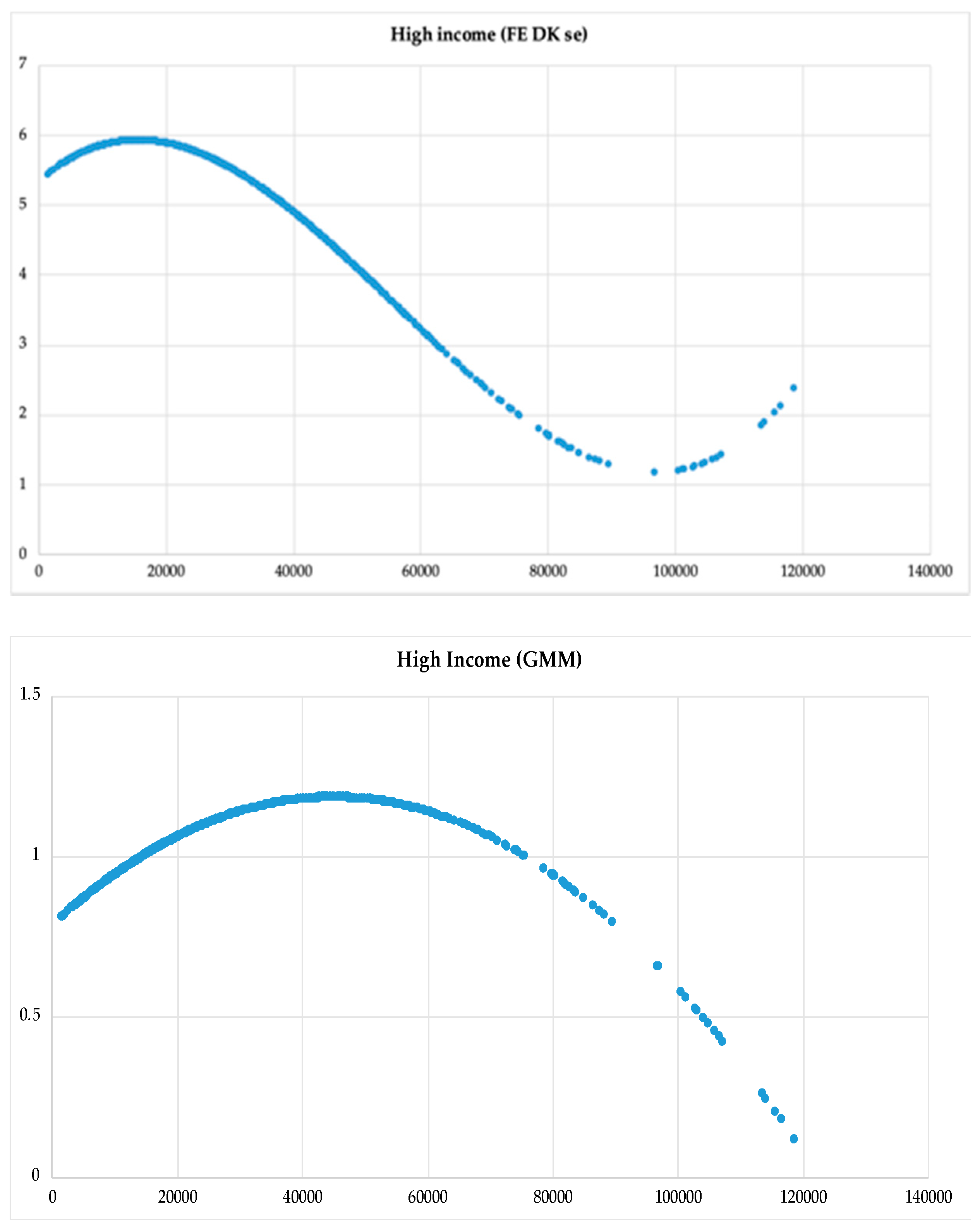
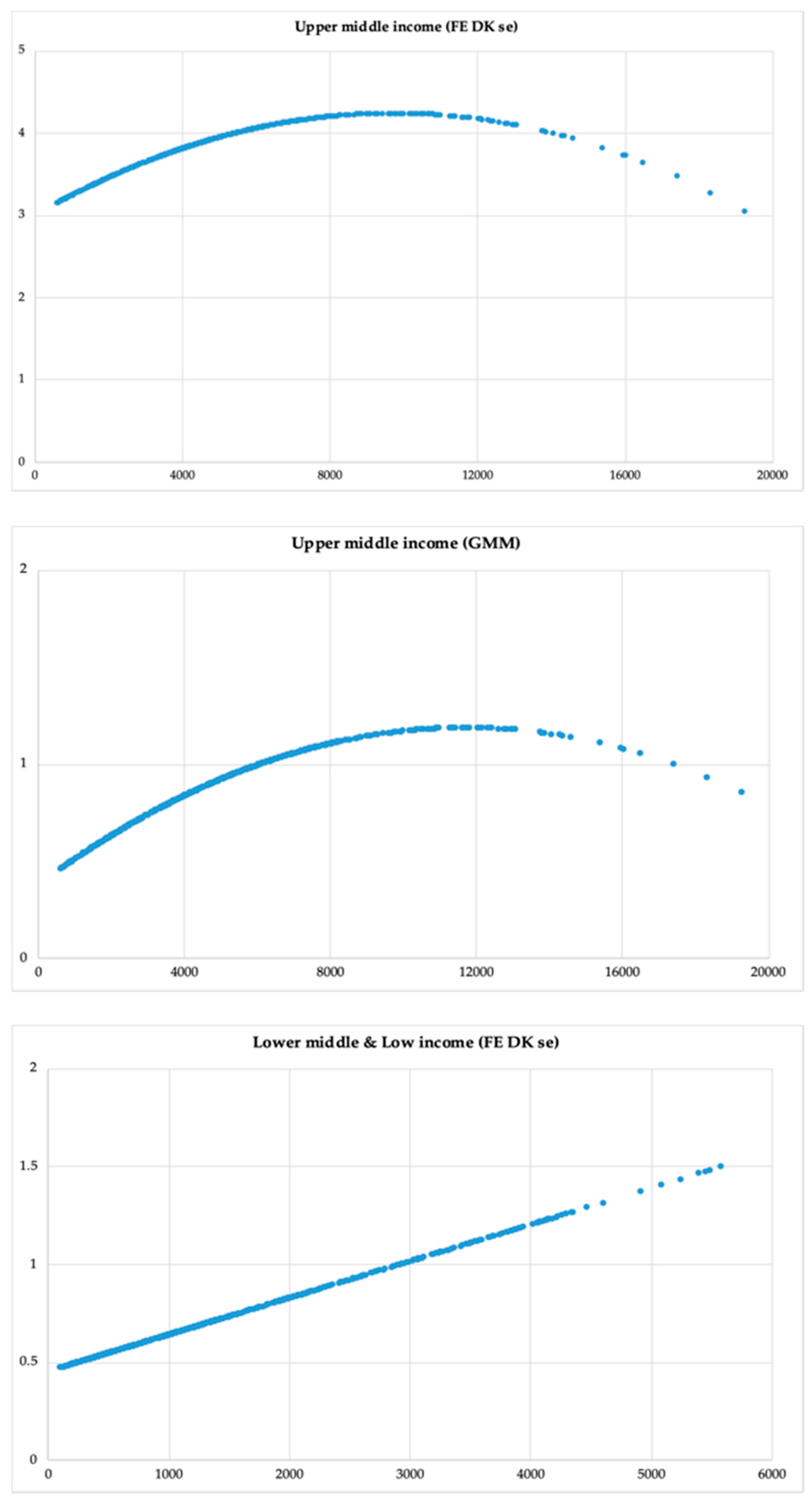
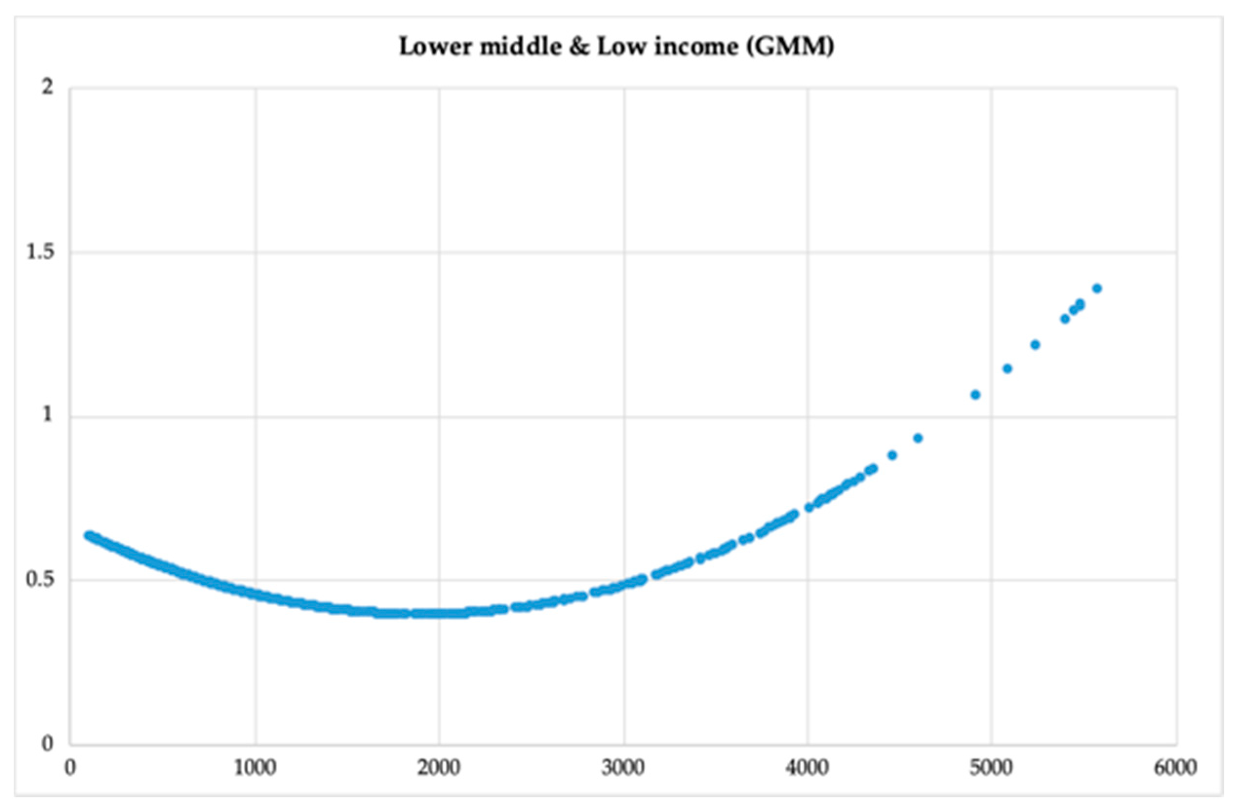
| Shape of curve | N–shape | InvertedU–shape | Inverted U–shape | Inverted U–shape | Line | U–shape |
| Turning points | 15859.25 56497.18 | 45177.67 | 9763.36 | 11754.69 | 1919.95 | |
| Observations | 893 | 799 | 627 | 561 | 741 | 663 |
| Null Hypothesis | High Income | Upper-Middle Income | Lower-Middle and Low Income |
|---|---|---|---|
| EPRpc does not Granger Cause EPFpc | 0.1435 [0.8663] | 0.84386 [0.4306] | 8.49424 *** [0.0002] |
| EPFpc does not Granger Cause EPRpc | 0.22982 [0.7947] | 1.66069 [0.1909] | 2.2018 [0.1114] |
| CO2pc does not Granger Cause EPFpc | 1.14026 [0.3203] | 5.78463 *** [0.0033] | 1.68477 [0.1863] |
| EPFpc does not Granger Cause CO2pc | 6.58308 *** [0.0015] | 0.2931 [0.7461] | 10.4235 *** [0.00003] |
| GDPpc does not Granger Cause EPFpc | 9.3199 *** [0.0001] | 0.78258 [0.4577] | 4.17817 ** [0.0157] |
| EPFpc does not Granger Cause GDPpc | 11.7925 *** [0.000009] | 5.672 *** [0.0036] | 5.40786 *** [0.0047] |
| Dens does not Granger Cause EPFpc | 1.90495 [0.1495] | 1.58869 [0.2051] | 1.27445 [0.2803] |
| EPFpc does not Granger Cause Dens | 7.17602 *** [0.0008] | 0.51733 [0.5964] | 4.85094 *** [0.0081] |
| CO2pc does not Granger Cause EPRpc | 0.112 [0.8941] | 0.90316 [0.4059] | 0.5376 [0.5844] |
| EPRpc does not Granger Cause CO2pc | 0.17197 [0.8420] | 0.39549 [0.6735] | 1.11302 [0.3292] |
| GDPpc does not Granger Cause EPRpc | 4.5241 ** [0.0111] | 0.85324 [0.4266] | 0.29639 [0.7436] |
| EPRpc does not Granger Cause GDPpc | 11.4263 *** [0.00001] | 0.65071 [0.5221] | 0.60933 [0.5440] |
| Dens does not Granger Cause EPRpc | 0.00811 [0.9919] | 2.22833 [0.1087] | 2.52252 * [0.0810] |
| EPRpc does not Granger Cause Dens | 0.0213 [0.9789] | 0.43188 [0.6495] | 0.0277 [0.9727] |
| GDPpc does not Granger Cause CO2pc | 5.4029 *** [0.0047] | 10.2292 *** [0.00004] | 4.74665 *** [0.0090] |
| CO2pc does not Granger Cause GDPpc | 3.1871 ** [0.0418] | 19.8117 *** [0.000000005] | 4.78144 *** [0.0087] |
| Dens does not Granger Cause CO2pc | 13.151 *** [0.000002] | 0.81525 [0.4431] | 0.55917 [0.5720] |
| CO2pc does not Granger Cause Dens | 3.64024 ** [0.0267] | 0.26402 [0.7681] | 1.38006 [0.2523] |
| Dens does not Granger Cause GDPpc | 0.60785 [0.5448] | 1.34882 [0.2604] | 5.72788 *** [0.0034] |
| GDPpc does not Granger Cause Dens | 1.38 [0.2522] | 1.70387 [0.1829] | 0.2997 [0.7411] |
| Observations | 799 | 561 | 663 |
Publisher’s Note: MDPI stays neutral with regard to jurisdictional claims in published maps and institutional affiliations. |
© 2021 by the authors. Licensee MDPI, Basel, Switzerland. This article is an open access article distributed under the terms and conditions of the Creative Commons Attribution (CC BY) license (http://creativecommons.org/licenses/by/4.0/).
Share and Cite
Halkos, G.E.; Gkampoura, E.-C. Examining the Linkages among Carbon Dioxide Emissions, Electricity Production and Economic Growth in Different Income Levels. Energies 2021, 14, 1682. https://doi.org/10.3390/en14061682
Halkos GE, Gkampoura E-C. Examining the Linkages among Carbon Dioxide Emissions, Electricity Production and Economic Growth in Different Income Levels. Energies. 2021; 14(6):1682. https://doi.org/10.3390/en14061682
Chicago/Turabian StyleHalkos, George E., and Eleni-Christina Gkampoura. 2021. "Examining the Linkages among Carbon Dioxide Emissions, Electricity Production and Economic Growth in Different Income Levels" Energies 14, no. 6: 1682. https://doi.org/10.3390/en14061682
APA StyleHalkos, G. E., & Gkampoura, E.-C. (2021). Examining the Linkages among Carbon Dioxide Emissions, Electricity Production and Economic Growth in Different Income Levels. Energies, 14(6), 1682. https://doi.org/10.3390/en14061682