Article

Self-Consumption and Self-Sufficiency in Photovoltaic Systems: Effect of Grid Limitation and Storage Installation

1
Energy Department, Politecnico di Torino, Corso Duca Degli Abruzzi 24, 10129 Torino, Italy
2
Department of Microelectronics, Technical University of Sofia, 8 Kliment Ohridski Blvd., 1000 Sofia, Bulgaria
*
Author to whom correspondence should be addressed.
Energies 2021, 14(6), 1591; https://doi.org/10.3390/en14061591
Submission received: 10 February 2021 / Revised: 9 March 2021 / Accepted: 10 March 2021 / Published: 12 March 2021
(This article belongs to the Special Issue Analysis of Solar Photovoltaic Self-Consumption)

Abstract

:
This paper presents a methodology to maximize the self-sufficiency or cost-effectiveness of grid-connected prosumers by optimizing the sizes of photovoltaic (PV) systems and electrochemical batteries. In the optimal sizing procedure, a limitation on the maximum injection in the grid can affect the energy flows, the economic effectiveness of the investments, and thus the sizing results. After the explanation of the procedure, a case study is presented, and a parametric analysis of the effect of possible injection limits is shown. The procedure is applied to size plants for an Italian domestic prosumer, whose electric load profile was measured for a year. A software program developed using the proposed methodology is also briefly presented. It is used for both research and educational purposes, both in laboratory classes and in remote lessons.

1. Introduction

In recent years, energy policies and the established urgency of reducing CO2 emissions have resulted in increasing progress in the generation of energy from renewable sources, such as photovoltaic (PV) systems, both in terms of implementation and in reducing its costs. This goal raises new challenges for national and international policy systems by addressing not only industrial or large-scale users, and therefore businesses, but also small users, namely households, in order to meet all or part of the needs of their energy demand. In this way, passive consumers, thanks to the process of self-consumption, i.e., on-site energy production and consumption, are gradually becoming active prosumers [1]. The presence of active prosumers has impacts on the network operation: it introduces new challenges and opens new scenarios, by introducing also novel roles for the system operators in the future [2]. Moreover, also the role of the prosumer as actively involved in the network operation must be taken into consideration, thanks to the implementation of new control systems [3] and novel measurement approaches (such as the net metering [4]), enabling the complete integration of intermittent energy sources in the system.
The self-production of electricity from renewable sources for self-consumption generates immediate positive effects, such as the reduction of grid energy losses, the mitigation of congestion problems, and a reduced need for modernization of electrical infrastructures by integrating renewable distributed generation into the electricity system [5]. Green energy, thanks to the growing success of self-consumption, therefore plays a strategic role of fundamental importance, creating a model of energy transition that aims to combine technological innovation and respect for the environment with employment benefits and economic, as well as health and environmental, advantages. In some countries, renewable electricity has reached grid parity, which means that the projected unit cost of self-generated electricity is equal to or lower than the unit cost of electricity obtained from the grid [1].
In future distribution systems, the high renewable penetration will increase peaks of generation. As a consequence, reverse power flows, i.e., the power coming from the distributed generation going to the distribution Medium Voltage/Low Voltage (MV/LV) transformer, will be high, with issues in the management of the grid [6,7]. For this reason, PV systems with low injection in the grid will be probably preferred in the future; in other cases, injections could be prohibited.
The present paper proposes a methodology to optimize the self-sufficiency and the self-consumption, or the economic return, of a PV storage system. However, with respect to most of the works in the literature, the effects for domestic users due to imposing different levels of limitation on the maximum injection into the grid are evaluated. In particular, an additional constraint regarding the maximum power injected into the grid is added into the optimization problem, and results are investigated. Furthermore, the impact of production and consumption profiles with different time steps is analyzed. Indeed, the energy outputs from simulations with different time steps are compared in order to determine the acceptable resolution of power profiles for the planning of PV storage systems.
The paper is organized as follows. Section 2 defines the concept of self-consumption and self-sufficiency and presents a brief review of the main strategies to maximize these quantities in the literature. Section 3 shows the procedure to simulate PV production and energy flows exchanged with the grid, useful to calculate the self-consumption and self-sufficiency. Section 4 presents a residential case study with the analysis of the variation in self-consumption and self-sufficiency levels and on the financial assessment in case of storage and curtailment in grid injection. Section 5 includes the conclusions.

2. Review of the Most Common Strategies to Maximize Self-Consumption and Self-Sufficiency

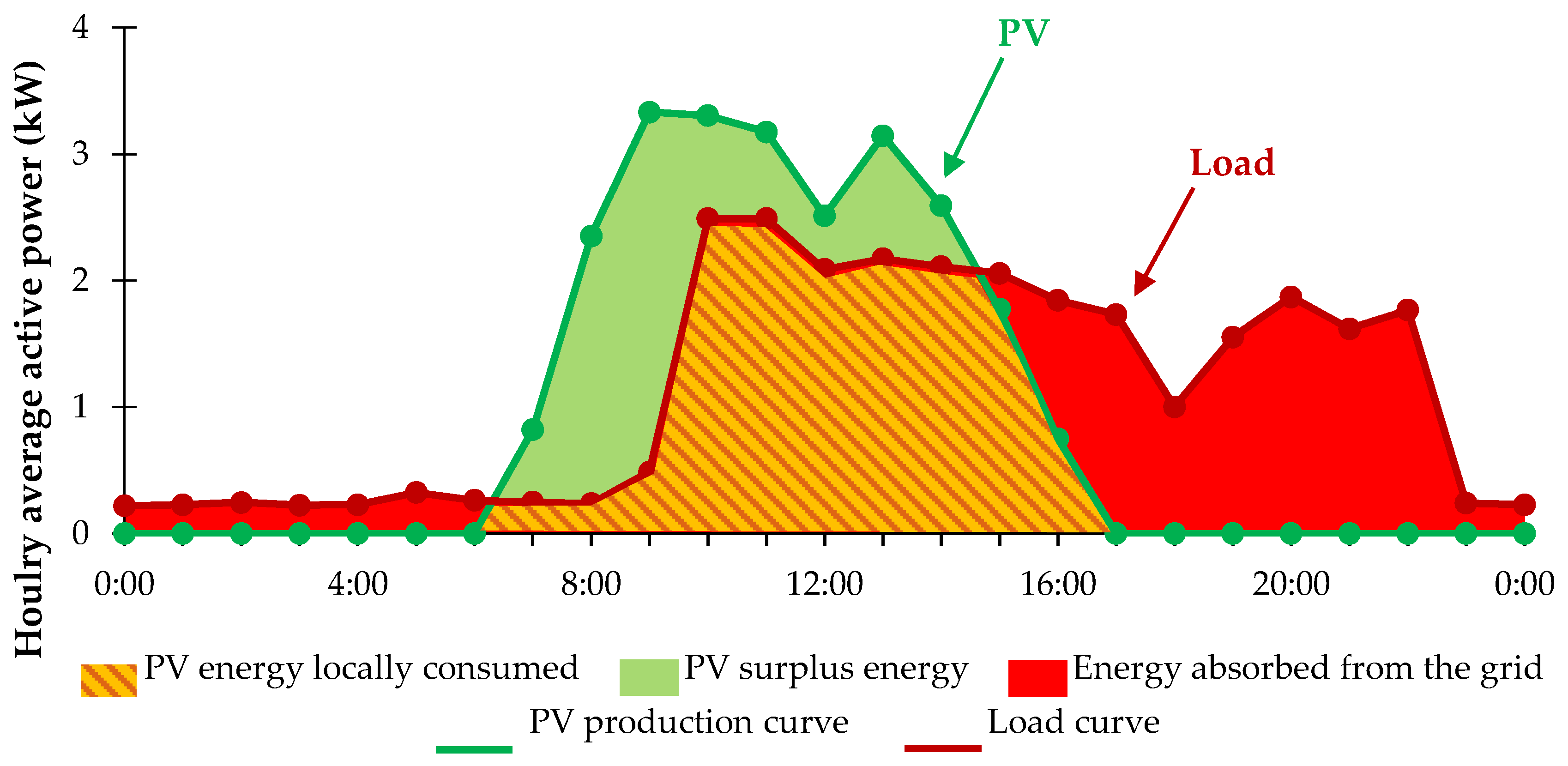
2.1. Definition of Self-Consumption and Self-Sufficiency

As stated in the Introduction, the proper integration of distributed renewable generators may benefit the entire energy system, and the use of the energy close to the production site contributes to the achievement of this goal. In this context, self-consumption and self-sufficiency are two energy indicators to quantify the exploitation of energy generation at local level.
The self-consumption (SC) is defined as the amount of electricity locally generated and consumed (Elgc) with respect to the total local generation (Egen) [5]:
S C x = E lgc , x E gen , x
where x is the time duration in which the ratio is calculated on a daily, monthly, and yearly basis.
The self-sufficiency (SS) measures the consumption amount supplied by local generation (Elgc the same numerator of the SC) with respect to the total consumption (Eload). It quantifies user independence from the grid [8] and it is calculated according to:
S S x = E lgc , x E load , x
Figure 1 shows an example of a generic domestic user with PV generation and load daily profiles with the aim of clarifying the difference between self-consumption and self-sufficiency. The yellow and orange striped area is the PV energy locally consumed, while the green area identifies the surplus energy generated by the PV system. The red area indicates the energy absorbed from the grid, i.e., the energy locally consumed from the grid. SC is given by the ratio between the PV energy locally consumed and the total PV generation. The total PV generation is the sum between the PV energy locally consumed and the surplus energy generated by the PV system. Instead, SS is the ratio between the PV energy locally consumed and the total load. The total load is the sum of the PV energy locally consumed (striped area) and energy absorbed from the grid (red area). In the example analyzed in the figure, SC and SS reach, respectively, 62% and 53% on a daily basis. Obviously, the values of SC and SS are subject to daily variations based on the different profiles of PV production and load.
Generally, production and consumption profiles rarely coincide: in this case, low values of SS or SC are obtained due to this mismatch. In case of surplus (generation higher than consumption), the unused Renewable Energy Sources (RES) production may be injected into the electrical grid or wasted, resulting in low SC. On the contrary, deficit condition (generation lower than consumption) occurs, causing energy absorption from the grid and low SS. The maximization of the SC, along with the SS, determines benefits for the users and the electricity grid.

2.2. Main Strategies to Maximize the Self-Consumption and the Self-Sufficiency

In the literature, many techniques are presented to achieve high levels of self-sufficiency and self-consumption. The most common solution to increase self-consumption and self-sufficiency is the integration of energy storage. An overview of the main energy storage technologies used in electric power systems is presented in [9,10]. The adopted technologies to store energy may vary, and their specific characteristics (duration, costs, energy density, charging/discharging power, and efficiency) vary as well. For example, batteries have a fast response (fractions of a second), while pumped hydroelectric stockpiles are able to store a higher amount of energy but they require a specific setting regarding the geographical location. The selection of the most adequate technology depends on the application: for example, recent works have investigated the integration of electric vehicles, which may perform similarly to stationary batteries, to increase prosumer self-sufficiency [11]. Nevertheless, it is possible to combine different typologies in the same system; however, in this case, it is fundamental to state their order of intervention. An energy storage aims to fill the gap between renewable energy source (RES) generation and load [12], mitigating grid instability and power quality issues [13]. Actually, the production and consumption profiles rarely coincide; thus, the energy produced may not meet the users’ needs. In case of surplus (RES generation higher than consumption), a part of the production is not exploited to fulfil the energy demand. This contribution can be stored in energy storage, if any, to increase the self-consumption, or can be injected into the grid. The first strategy, named “peak shaving”, adjusts the production (production peak shaving, PPS) or the consumption profiles (demand peak shaving, DPS), obtaining a total match without injecting into the grid. For industrial customers [14,15], residential applications [16], and tertiary users [17], electrochemical storage is recommended to shave the production and consumption peaks. Moreover, the same effect may be achieved without storage systems.

2.3. Description of Peak Shaving Techniques without Energy Storage

In the case of PPS, the energy generated by RES is reduced in order to avoid overload and overvoltage events and to provide a valuable benefit to the electricity grid [18]. In the literature, many strategies are described to reduce the energy surplus of wind generators [19,20,21]; for example, the selected orientation of the turbine blades may not be the optimal one. Regarding PV systems, their energy reduction is performed by modifying their operating point; in particular, they are forced to work not in their maximum power point (MPP) in the current-voltage characteristic [22]. These solutions are the simplest, but not the most efficient; indeed, they do not take into account the energy balance with local loads and battery operation.
In the case of DPS, the peak load is reduced: the exploitation of expensive peak generation systems (such as fossil fuel plants) is avoided. This condition allows better forecasting and easier management of the electricity grid, increasing the safety of supply for the users. Moreover, energy suppliers provide economic incentives to users in order to lower their peak loads [23]. Examples of DPS are proposed in [24,25].

2.4. Review of Methodologies Maximizing Self-Consumption or Self-Sufficiency

In the literature, many methodologies are used to maximize the self-consumption or the self-sufficiency of RES systems. One paper [26] proposes a methodology to optimize the levelized cost of electricity and the pollutant emissions of an RES-based microgrid. However, the paper shows that the solution corresponding to the maximum self-sufficiency leads to a huge overcapacity of RES generation. Thus, this solution does not coincide with the optimal one from economic and environmental points of view. In [27], a methodology is proposed to evaluate the energetic/economic performance of prosumers with PV modules and electrochemical storage, maximizing their self-consumption and sufficiency. In [28], the integration of PV arrays on the roof and façades of a building in France is optimized, maximizing the self-consumption of the building. In particular, three mono-objective optimizations are performed, with different objective functions. However, a global optimization for PV design, taking into account these factors, is not analyzed and batteries are not included in the work. In another paper [29], the self-consumption and the self-sufficiency for a supermarket in Germany are optimized, with sensitivity analyses of the main parameters in the PV storage system (cost, size, and interest rates). Another work [30] investigates the optimal PV battery configuration in terms of self-consumption/self-sufficiency and economic savings using a two-step assessment.
In such methodologies, limits on maximum injection into the grid are not included: peak shaving strategies are integrated in the analysis using storage systems only (electrochemical batteries or the water catchment area of hydropower plants). For sites with favorable weather conditions, during sunny days, RES generation may be much larger than electric consumption. In this case, the surplus energy produced may be stored in the batteries or other storage facilities. However, their energy capacity is limited: if surplus energy may be still exploited but the maximum state of charge is reached, this energy cannot be stored, being injected into the grid. Actually, domestic users have specific contracts with grid operators, and their economic costs are affected by the maximum power that prosumers may inject into the grid. In this context, users may want to install RES systems without modifying their contracts, or they may wish to increase this value (thus, the economic expense of the contract) up to a specific value. On the contrary, in some countries [31], grid operators may not accept power injection into the grid in order to improve its stability and reliability. In this case, if the storage is totally charged, the surplus energy from RES generators is wasted. The present paper proposes a procedure to maximize self-sufficiency/self-consumption or the economic return. However, with respect to most of the works in the literature, it investigates different levels of limitation on the maximum injection into the grid from domestic users, evaluating the energy and economic benefits for the prosumers. In particular, an additional constraint regarding the maximum power injected into the grid is added in the optimization problem, and results are investigated.
Other works, including [32,33], contain procedures aiming to optimize the integration of RES-distributed generators into the electrical grid; effective peak shaving strategies are considered in the analysis, but they are related to the demand (DPS).

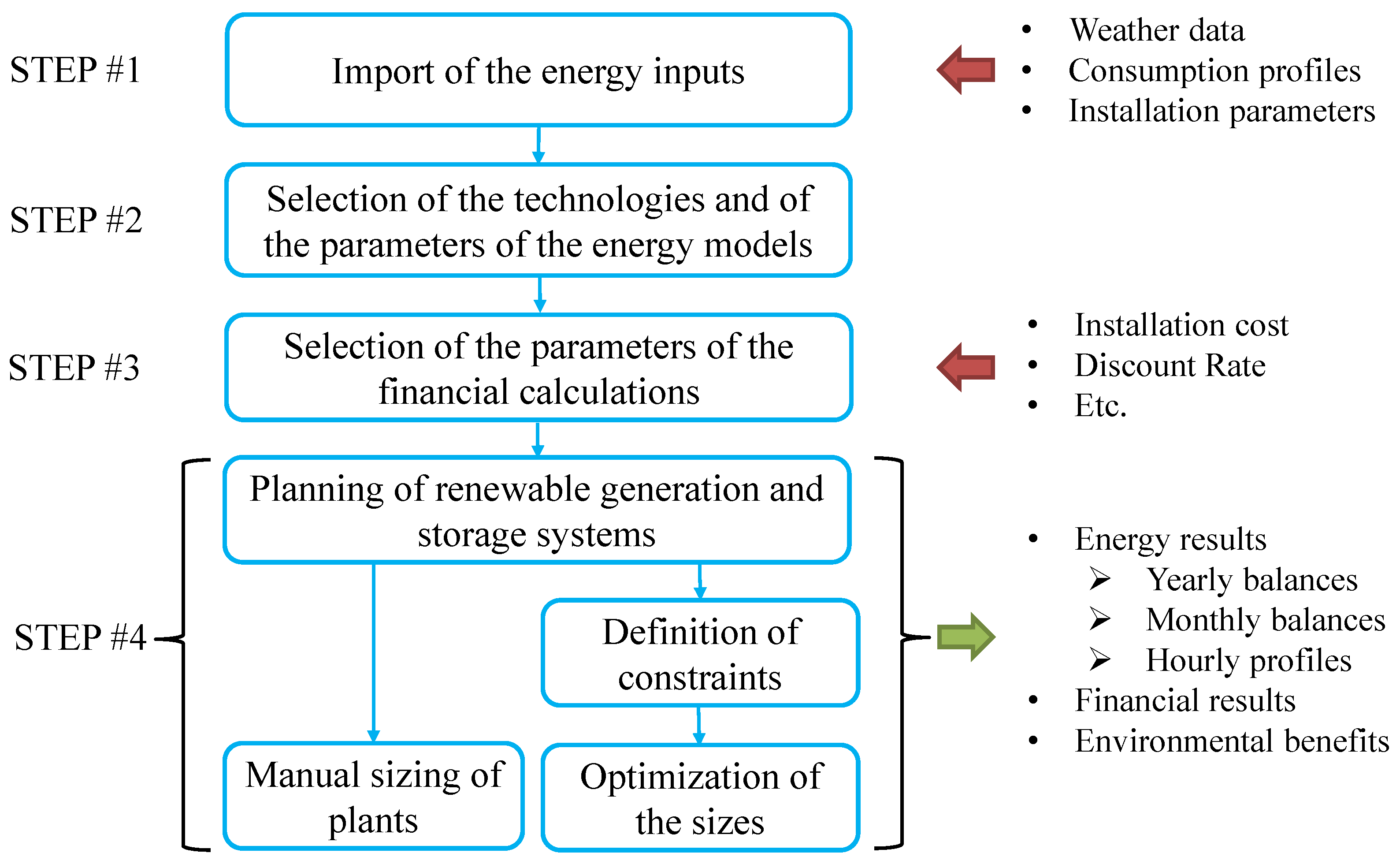
3. A Methodology for the Optimal Sizing of PV and Batteries

The proposed procedure aims to optimize the self-sufficiency or cost-effectiveness of grid-connected prosumers equipped with intermittent RES generators and electrochemical storage. The simulations can be performed for plants of any size. The present work focuses on PV systems and electrochemical batteries. The procedure is described step by step in the following subparagraphs. For the sake of clarity, the corresponding flow chart is shown in Figure 2.

3.1. STEP #1—Import of the Energy Inputs

Different weather databases exist [34,35]; above all, the Photovoltaic GIS database (PVGIS), from the EU Commission, is one of the most used. It contains data about solar radiation, air temperature, and wind speed for large areas of the world. The user has to select the site in which the simulation and planning of PV, Wind Turbines (WTs), and storage will be performed. The weather data consist of profiles for an entire year for solar irradiance (kW/m2) on a surface with a defined tilt and azimuth, air temperature (°C), and wind speed (m/s) at a defined measurement height. Regarding the time step, PVGIS provides hourly profiles. Nevertheless, the proposed procedure works also with smaller time steps, according to data availability and the accuracy required by the analysis.
In addition to the data related to generation from renewables, the consumption profile has to be included to compare them, simulate the storage operation, and calculate the exchanges with the electrical grid. In order to obtain the load profiles, a possible solution is to measure actual consumption profiles by using meters or to find typical consumption profiles (e.g., from [36]).
Energy balances between PV generation and electrical consumption are often performed using profiles with 1-h time steps [37,38]. In fact, in most applications, hourly profiles are easier to obtain, requiring a lower computational cost with respect to data with lower time steps, e.g., from seconds to minutes. The impact of time resolution (up to 1-h values) becomes almost negligible for the planning and sizing of PV systems in the case of storage installation. In particular, the optimal PV-rated power is not affected by time resolution, while the sizing of batteries may be affected by negligible errors (up to ≈2% in the case of 1-h time steps). Moreover, the estimation of yearly savings on the electricity bill is not affected by time resolution either [39]. In [37], it is analyzed how the presence of storage reduces the error on yearly SC and SS evaluation, taking into account profiles with time steps from 15 min to 1 h. With respect to 15-min profiles, hourly data introduce errors lower than 1%. Obviously, if the goal of the study consists of a detailed analysis of power flows, SC, and SS within the hour, the use of data with lower time resolution is required. In particular, load profiles with a time step below 30 s and PV profiles with 10-min resolution or above are suggested for PV systems without storage. On the contrary, if batteries are installed, load profiles with a minimum resolution of 5 min are recommended [40,41].
In the present work, the procedure to find the optimal size of PV and storage is based on the comparison between yearly SC, SS, and NPV values of different configurations; the used profiles have 1-h time steps.
Figure 3 (top chart) shows an example of consumption and generation profiles for a household in North Italy. Profiles are shown for an entire day, and they are measured with a time step of 5 min. The 5-min profiles are averaged to obtain 15-min and 1-h profiles; their graphs are shown in the middle and in the bottom of Figure 3, respectively. Injections and absorptions from the grid are also shown; in every case, they are calculated as result of the balance between generation and load.
The comparison of the profiles demonstrates that a lower time resolution leads to a reduction in consumption peaks and in a mitigation of generation fluctuations. As a result, the obtained smoother profiles lead to overestimations of SC and SS. The overestimations related to the profiles in Figure 3 are quantified in Table 1. The SS is 56% in the case of 5-min measured data; it increases to 57% for 15-min profiles and reaches 61% for hourly profiles. The relative deviation with respect to the measured profiles is ≈2% and ≈10%, respectively. The same relative deviations also occur for self-consumption.
The same analysis is performed on an entire year and results are presented in Table 2. Obviously, during both a single day and the entire year, the consumption and production energies do not change when varying the time step of the profiles. The difference is in the balance among them, leading to different exchanges with the grid. For example, moving from 5-min to 1-h profiles, the injection into the grid decreases by 7%, while the absorption decreases by 5%; as a result, the yearly relative increment for both self-sufficiency and self-consumption is ≈9%.
It is worth noting that in most countries, the balance settlement period is 1 h. In Europe, the European Commission is working towards the harmonization of the balance settlement period, imposing a common value of 15 min [42]. The imbalance within 15 min is compensated by the electric grid, which can be considered by the prosumer as a storage facility with infinite capacity. Thus, 15-min profiles should be used as a reference for the calculation of the energy results. In the case study presented in Table 2, the grid injection is 3254 kWh/year with the 15-min profiles, and it decreases to 3102 with 1-h profiles (−4.7%). The grid absorption decreases from 4238 to 4087 kWh/year (−3.6%). As a result, the relative deviation in SS and SC is ≈6% between 15-min and 1-h profiles. In conclusion, the proposed methodology is slightly affected by the use of hourly time steps, and it can be used for planning purposes.

3.2. STEP #2—Selection of the Technologies and of the Parameters of the Energy Models

Regarding the photovoltaic technology, the production is evaluated according to the model described in [43]. In particular, PV power is proportional to irradiance G by means of the PV efficiency ηPV. However, ηPV has a nonlinear dependence on irradiance: in fact, a PV system requires a minimum irradiance (a threshold irradiance G0, which is around 17 W/m2) to generate power. Thus, PV efficiency can be calculated starting from the rated efficiency in standard test conditions (STC, corresponding to irradiance GSTC = 1000 W/m2 and module temperature TSTC = 25 °C), as follows:
η PV ( G ) = η STC · G G 0 G · Π η with   Π η = η th · ( 1 ξ mix ) · η DC / AC
where ηSTC is a function of rated power at STC PSTC, of irradiance GSTC, and of the PV surface APV (ηSTC = PSTC/(APVGSTC)), and it is ≈21% in actual commercial modules. The quantity Πη is an equivalent efficiency calculated as the product of the thermal efficiency (ηth), the efficiency in the DC/AC conversion (ηDC/AC), and the other so urces of losses (1 − ξmix) ≈ 92%. In particular, ηth can be estimated as:
η th ( T c ) = 1 + γ · ( T c T STC )
where γ is the thermal coefficient for power, which is provided by the manufacturer, and it ranges between ≈−0.45 and ≈−0.35%/°C [44,45], and Tc is the module temperature.
The effect of temperature on PV efficiency is shown in Figure 4a; increasing temperature leads to worse PV efficiency. Moreover, the DC/AC efficiency is a nonlinear term as well (Figure 4b), because it depends on the load factor, which is the ratio between the actual PV power and the maximum value.
In particular, the efficiency of DC/AC conversion increases with the load factor, reaching a value up to ≈99% at full load in the most recent commercial devices. Finally, ξmix ≈ 8% is a miscellaneous factor that takes into account losses due to dirt, glass reflection, Joule effect in cables, and the MPP tracking.
PV manufacturers guarantee the efficiency ηSTC to be at least higher than 80% after 20 years, corresponding to a linear decrease of −1%/year. However, in recent years, several experimental campaigns have stated that the degradation of crystalline silicon modules may be lower, if there are no damages. In particular, in the present paper, the decrease has been assumed to be −0.5%/year [46,47].
As a result of the above-described model, it is possible to calculate, for each time step, the electricity production from PV arrays of whatever size; thus, it can be calculated the productivity YPV of the generator, e.g., the annual energy production per unit of power installed in kWh/kW/year.
Regarding storage modeling, the performance of batteries is described by the state of charge (SOC) estimation, because it is an adequate compromise between accuracy and simplicity [48]. In particular, the SOC at a time ti can be evaluated as a function of the SOC at the previous instant ti−1 (SOCti−1) [49]:
S O C ( t i ) = S O C ( t i 1 ) P bat ( t i ) · Δ t C E , bat P b a t > 0
S O C ( t i ) = S O C ( t i 1 ) η bat · P bat ( t i ) · Δ t C E , bat P b a t < 0
where Pbat is the average power exchanged between the batteries and the system in the time step Δt (Pbat is assumed negative in charging phase and positive during discharge), ηbat is the charge/discharge efficiency of the storage in charging operation, and CE,bat is the energy capacity of the storage facility. The performance of batteries decreases over time due to degradation: their state of health (SOH), which is the ratio between actual energy capacity and rate value [50], decreases while cycling and the manufacturer provides two additional limits in order to avoid too low values of SOH. In particular, the manufacturer provides a maximum number of cycles and a maximum number of operating years: the replacement of batteries is recommended after exceeding the minimum between the two limits. For the sake of clarity, an example is provided. For commercial lithium batteries for stationary purposes, a typical maximum age before replacement is 10 years, and the maximum number of charge–discharge cycles is equal to 10,000 [51]. Supposing a single charge–discharge cycle per day (average value), during one whole year, the storage performs 365 cycles, and after 10 years, it is 3650. This value is lower than the 10,000, but the battery is substituted, because it worked for 10 years. On the contrary, in the case of five cycles per day, after 6 years, the battery has performed 10,950 cycles and has to be changed. In the proposed methodology, dynamics for frequent charging and discharging are not investigated. Actually, the safety parameters provided by manufacturers (maximum/minimum SOC, maximum power) are respected. Moreover, the replacement of batteries after their lifetime is performed to avoid a huge decrease in their SOH over time.
The converters also have a shorter life than the PV modules; they are substituted after 10 years.
Regarding the logic to control the charge–discharge of batteries, in the present study, it works as follows. The energy from the storage has priority over energy from the grid in meeting the energy demand, when production from renewables is not sufficient. In the same way, first, batteries are charged; then, energy is injected into the grid. Other discharge logics, also depending on PV production forecast, can be integrated into the proposed procedure depending on the goal to be achieved [52].
In addition to the simulation of PV systems and batteries, it is also possible to include other typologies of renewables, such as wind power systems. For such generators, the calculation of their produced energy requires the wind speed profile of the site under study and the “wind speed–power output” relationship, or power curve, of the selected turbine [53]. Then, the wind speeds are corrected to the height of the turbine hub and the resulting values are used in the power curve to obtain the corresponding output power [48].

3.3. STEP #3—Selection of the Parameters for the Financial Calculation

Regarding the economic analysis, the parameters to be calculated are the net present value (NPV) and the internal rate of return (IRR). In particular, the NPV can be calculated as follows [54]:
N P V = C I n = 1 N C ( 1 + i ) n + n = 1 N R ( 1 + i ) n
where N is the expected lifetime of the system, n is the number of years, i is the discount rate, CI is the investment cost, C is the absolute value of the negative cash flow for the nth year, and R is the positive cash flow for the nth year. In the case of PV and battery systems, the negative cash flow C includes planned maintenance and extraordinary maintenance, e.g., replacement of batteries, inverters, or damaged PV modules. The positive cash flow (revenue) R takes into account the earnings from the sale of electricity injection into the grid. In the case of prosumers, the self-sufficiency reduces the absorption from the grid; thus, another positive cash flow is the saving due to a lower electricity bill. In the case of economic incentives (e.g., tax discounts) or feed-in tariffs, they can be taken into account.
The IRR is the discount rate that permits the NPV to be set equal to zero, i.e., it permits the costs of the system to be counterbalanced, after its lifetime. As suggested in [55], investment in renewables with IRR > 6% can be considered acceptable.
In addition to the financial parameters, the literature presents different environmental factors that can be included. Among all of them, the avoided CO2 emission, the energy payback time, and the life cycle conversion efficiency are the most important [56].

3.4. STEP #4—Planning of Renewable Generation and Storage Systems

The proposed sizing of plants and storage is an iterative top-down analysis. First, the user decides on the goal. For example, generators and storage could be sized to better match the load without increasing too much the exchange with the grid [57], or the goal could be the highest economic return. In these cases, the analysis should start with the selection of reasonable starting sizes. The generators have the priority. The starting size is the value that permits the production of the equivalent of the annual load. In the case of PV systems, it can be calculated as the ratio between the productivity of the plant YPV and the electric load. Regarding storage, a reasonable starting size can be that to store the daily requirement from the load. It corresponds to the average daily consumption of the user during the year.
After the definition of the starting values, the PV production profile can be generated according to the models described in the previous subparagraph. Production profile has to be compared with the load. For each time step, the operation of the battery is calculated and the SOC is updated. Batteries cannot always balance production and load: in this case, the remaining surplus or deficits between load Eload, generation Egen, and battery charge/discharge Ebat are the injections and absorptions from the grid Egrid (with the generation convention):
E gen + E bat + E grid = E load
with
Ebat > 0 during battery discharge;
Egrid > 0 during absorption from the grid.
After performing the energy balance for each time step of the simulation, power flows have to be integrated to obtain yearly quantities. The analysis of yearly results permits an overview of the situation. The main yearly energies to be computed are the total production from renewables, the load, storage charge and discharge, the quota of energy locally produced and consumed, injection into the grid, and absorption from the grid. On the basis of these quantities, self-sufficiency and self-consumption levels can be calculated. In the case of low self-sufficiency, the reason could be an undersized plant or a bad match between load and generation.
The bad match could be at seasonal level or on a daily/hourly basis. The check of monthly quantities shows immediately if there are seasonal differences. For example, in the case of a domestic prosumer with a PV installed on the rooftop, high production can be generally expected in summer, with a very low contribution in winter. In this case, the prosumer could install a generator with different tilt and azimuth, to change the seasonal production [58]. Another possible solution is a heterogeneous portfolio of generators (e.g., PV, wind, hydro), which could help in achieving a better seasonal match [59]. The analysis of daily profiles permits the mismatch to be studied. It has to be performed with a time step of hours or less, depending on the accuracy required for the results [40]. For example, PV generation is concentrated in sunlight hours, but domestic loads generally occur during early morning and evening (typical for families with working people not at home in the central hours of the day). In this case, the increase in batteries can reduce the day–night mismatch, and/or the load shifting should be applied.
Figure 5 shows a generic example of a graph to be generated in order to study the daily balances. It shows an aggregated hourly generation profile from WTs and PV plants, along with load profiles and storage operation during a summer day. The storage is charged in the morning (when production is higher than the consumption). When it is full (at 9:00 a.m.), the surplus is injected into the grid. In the evening (after 9:00 p.m.), PV modules are not active and only WTs generate power; however, production from renewables cannot supply the entire consumption and the storage is discharged.
In this case, the energy contained in the storage is not enough to supply the loads and grid absorption is required. The same analysis should be performed on a typical day during the other seasons. Based on the analysis of these results, the user decides how to change the portfolio of generation and storage.

3.5. Considerations Related to the Optimization Criterion

The sizing of generators and storage may be performed to obtain different goals. In the present work, the two optimizations aim to maximize two objective functions Γ: the self-sufficiency (Γ1) and the economic return (Γ2), respectively. They are defined according to Section 2.1 and Section 3.3, respectively, and the optimization variables are the size of PV system (PPV) and the energy capacity of batteries (CE,bat):
max   [ Γ 1 ( P PV ,   C E , bat )   ]   o r   max   [   Γ 2 ( P PV ,   C E , bat ) ]
with
IRR > 6%
PinjPinj,limit
0PPVPPV,max
0CE,batCE,bat,max
This definition of the objective function may be extended to other renewable systems, such as wind power plants; in this case, the new extended objective functions also depend on the main variables of these systems (e.g., the nominal power of the wind turbine to be installed).
The constraints of the optimization are twofold: the first one consists of setting IRR > 6%, which is a reasonable value to guarantee the cost-effectiveness of investments. This limit automatically guarantees a positive net present value. The second constraint is the limit Pinj,limit to the injection into the grid Pinj, i.e., the maximum power that may be injected into the electricity grid for a specific site. As described in Section 2.4, the proposed methodology takes into account the adoption of peak shaving strategy on generation profiles in order to increase the energy and economic benefits for the users. The effect of different values of Pinj,limit is investigated by a sensitivity analysis: different injection limits are imposed, and, for each case, the optimal sizes are calculated and compared.
Regarding the limitations of the optimization variables, the maximum limits required by the algorithm PPV,max and CE,bat,max are always selected to be far from the optimal values.
The aim of the first goal is producing as much energy as possible while avoiding too high exchanges with the grid. For this purpose, the maximization of the self-consumption is not suitable, because high levels of SC can be obtained with undersized plants, which do not decrease significantly the energy dependency from the grid. Indeed, a high amount of energy could be absorbed from the grid even with the highest SC rate. On the other hand, a high SS could be obtained with the installation of an oversized generation plant, which causes high energy injection in the grid. Thus, both SS and SC must be high.
The second goal considered in the present work is the cost-effectiveness; it is affected by the price of electricity sold to the grid, and by the economic value of self-consumed electricity. If the electricity sale is more profitable, the result of the economic return maximization will be an oversized generation system. On the other hand, if self-consumption is more profitable, while grid injection is paid little (as in Italy), the generation system will be sized on the basis of the user’s annual consumption.
In this work, the nonlinearity of the optimization problem is due to the financial analysis. In particular, Equation (7) permits the evaluation of the NPV, which is one of the objective functions (Γ2) in the paper. Moreover, one constraint of the optimization is related to the IRR, which is evaluated according to the following implicit formulation:
C I n = 1 N C ( 1 + I R R ) n + n = 1 N R ( 1 + I R R ) n = 0
where
C I = f ( P PV ,   C E , bat ) ,   C = f ( P PV ,   C E , bat )   and   R = f ( P PV ,   C E , bat )
The dependence of the NPV and the IRR on the optimization variables (the size of PV system, PPV, and the energy capacity of batteries, CE,bat) is implicit. Actually, these variables impact on the NPV and the IRR by affecting the energy exchanges of the system and its cash flows. In this context, the optimization problem is solved using sequential quadratic programming (SQP). It is an iterative algorithm that, at each iteration, approximates the nonlinear problem as a quadratic one, linearizing the equality/inequality constraints. The SQP is one of the best choices for constrained optimization problems because it does not require high computational cost, providing comparable accuracy with other nonlinear programming algorithms [60]. In order to check the correct operation of the SQP, the results were also calculated by following an exhaustive but with slow calculation of the results of all the possible sizes of PV and storage. It consists of an iterative method. Actually, the initial ranges and the discrete steps for the variables are large, while they become lower when solutions approach the optimum one. The result of this analysis demonstrates the correct operation of the SQP algorithm.

3.6. Application of the Procedure in a Software Program for Research and Remote Teaching

The proposed methodology was integrated into a software program that is currently used in the course “Power Generation from Renewable Sources” for students of Politecnico di Torino, and in e-learning courses [61,62] of the project “Euro-Mongolian cooperation for modernization of engineering”. This project, coordinated by the Technical University of Sofia, started in 2018 and it is funded by the European Commission (the partners are four European universities/institutions—Technical University of Sofia as the coordinator, Politecnico di Torino, Technical University of Berlin, National Institute of Solar Energy from France—and three Mongolian universities—National University of Mongolia, Mongolian University of Science and Technology, National Technical University) in the framework of “competence building in higher education”. The goal of the project is the modernization of electrical and electronic engineering curricula in Mongolia. E-learning courses are created within the project and they aim to provide new opportunities for cooperation between Mongolian and EU universities. Thus, features that encourage effective learning in both frontal and remote lectures are required. In order to permit the worldwide use of the software, it is realized in the form of an “.xls” spreadsheet file, which is the most common format for calculations. This extension can be used by third-party applications, available for every operating system. The “.xls” file can be downloaded and used also in offline configuration. In order to avoid the presence of dangerous software, the spreadsheet file does not contain macros, i.e., code in visual basic language. Thus, all the calculations are performed using spreadsheet formulae. In this way, students can access all the calculations performed in the software without knowing programming codes.

4. Case Study for the Calculation of Self-Consumption and Self-Sufficiency

A case study is used to better explain the proposed procedure. The case study deals with a residential user in Northern Italy. It will be equipped with a PV system, which could be coupled to a battery energy storage system (BESS). The correlation between PV plant size, self-sufficiency, self-consumption, and economic return is investigated. Then, the maximization of the self-sufficiency or of the economic return is carried out, in compliance with economic and technical constraints. Finally, the impact of the change in BESS investment cost on the self-sufficiency maximization is analyzed. To account for the rules of power generation curtailment (see Section 2.4), the calculations are performed for different values of power injection limits.

4.1. Calculation Inputs

The analyzed residential user is located in the province of Turin (Piedmont), with an annual electrical consumption of around 7000 kWh. This value is higher than the average annual electricity consumption for Italian families of four, which is ≈3000 kWh [63]. This is due to the electrification of users’ energy consumption for cooking, domestic hot water (DHW) production, and heating. Indeed, the consumption of an induction cooktop and of an electric heat pump adds up to that one of the classic household appliances, such as a refrigerator, washing machine, dishwasher, or lights. The use of induction cookers causes electricity consumption peaks from 12:00 to 14:00 and from 18:00 to 20:00, during the main mealtimes. An electric heat pump, characterized by a nominal power of 3 kW, is used to produce DHW. In addition, it contributes to satisfying the heating demand, for non-rigid external air temperatures (higher than 5 °C). In the case of lower external temperatures, a natural gas boiler is used.
The monthly electricity consumption of the user is strongly affected by the heat pump (Figure 6). They are high in the mid-seasons, because the heat pump is used for both DHW production and heating. Indeed, the consumption reached the highest annual values in March (797 kWh) and November (723 kWh). Instead, loads in the winter months are between 600 and 700 kWh/month, since most of the heating demand is fulfilled by the gas boiler. Lastly, summer consumption is below 400 kWh/month, as the heat pump deals only with DHW production, reaching a minimum consumption of 335 kWh in July.
In Figure 7, load profiles of a day in February and July are presented. The energy consumption is higher in February due to space heating and hot water production by the heat pump, while in July, peaks are due to induction platers, oven use, and hot water heating. Thanks to high external temperatures, the water heating requires a lower amount of energy with respect to February. Consumption profiles are measured using a commercial meter, adequate to measure the nominal AC voltage of 230 V and a current up to 45 Amps. The accuracy is 0.5% for both voltage and current, and 1% for power. The meter has an RS485 port for remote communication, and it is connected to a personal computer to store the data.
Solar irradiance and air temperature hourly data were downloaded from PVGIS. To calculate the PV production, the irradiance on a south-oriented surface inclined by 30°, an optimal slope for Northern Italy, was used. In the selected site, a surface with these features is characterized by an annual irradiation of ≈1500 kWh/m2 and an annual productivity of ≈1200 kWh/kW per year.
This case study does not represent the best situation in Italy. From the point of view of productivity, it is lower than in Southern Italy, where it can exceed 1500 kWh/kW·per year with the same installation conditions. Regarding the load, the analyzed prosumer uses heat pumps for heating purposes, with higher consumption from November to April, when the solar source is lower. On the contrary, in Southern Italy, the heating load is low, while the use of heat pumps is higher in summer for cooling. The good match between solar source and cooling load leads to higher values of self-sufficiency. Regarding the financial parameters, as described in the next subparagraphs, the differences are negligible.

4.2. Financial Parameters

The economic calculations carried out are valid for the country of Italy. The installation cost of the PV system was set to 1800 EUR/kW, typical of domestic plants up to few tens of kW, and its O&M cost was supposed to be 10 EUR/kW/year. The installation cost of Li-ion batteries was assumed equal to 300 EUR/kWh [42] and their charge efficiency was assumed equal to 90%. Their replacement occurs after exceeding 10,000 cycles or after 10 operation years. The DC/AC converters’ replacement occurs after 10 years. In Italy, currently, there are no feed-in tariffs for new PV plants of a few kW (lower than 20 kW) [64]. However, PV plants with a nominal power lower than 500 kW can access a net billing service called “Scambio sul posto” (on-site exchange). According to this service, the grid is used as a virtual storage facility for the electricity that is produced but not locally consumed by the user. It is a particular form of self-consumption that compensates for the electricity generated and injected into the grid at a certain time with the electricity that is absorbed from the grid and consumed at a different time [65]. Through the monthly electricity bill, the prosumer pays for the electricity absorbed from the grid. However, with renewable generation, the bills are lower due to self-consumed (or battery-stored) electricity, which is not measured by the electricity meter. At the end of the year, the energy service operator refunds the user with an economic contribution, which is the sum of two terms: the minimum economic value between the annual absorbed and injected electricity, and the cost of the use of the grid related to the minimum energy between absorption and injection.
In the case study, both the absorbed and injected electricity were valorized at the same price (0.11 EUR/kWh). Instead, the surplus electricity, i.e., the energy produced but not self-consumed, is sold to the grid at 0.04 EUR/kWh [66].
In addition to these positive annual cash flows, there is the saving related to the direct use of the self-generated electricity and to the deferred self-consumption through the BESS. This saving is equal to the avoided purchase of electricity from the grid, the cost of which is 0.20 EUR/kWh [67]. Thus, self-consumption is more convenient than using the grid as virtual storage (on-site exchange) or selling electricity to the grid. Another saving is related to the annual tax reduction: for the case study, it is set to 5% of the initial investment of the PV plant and the BESS, and it lasts 10 years.
In order to explain the net billing mechanism, a general example of its application is reported in Figure 8 without considering tax reduction. A user’s annual electricity consumption (Eload) is 7000 kWh and their PV system produces EPV = 7300 kWh/year. The self-consumption is 40%; the energy locally produced and consumed (Elgc) is 2920 kWh. At the end of the year, 4380 kWh is injected into the grid, while 4080 kWh is absorbed from the grid.
The annual net injection (Esurplus) in the grid is equal to 300 kWh. The economic values of injection and absorption flows are, respectively, EUR ≈ 482 and EUR ≈ 449 (0.11 EUR/kWh); thus, GSE pays EUR ≈ 449 to the user. In addition, EUR 12 are obtained from the sale of Esurplus to the grid (0.04 EUR/kWh), resulting in a total annual gain of EUR ≈ 461. The saving on the electricity bill is given by the avoided purchase of Elgc from the grid at 0.20 EUR/kWh (EUR 584): the passive user pays EUR 1400 (7000 kWh with a unitary cost of 0.20 EUR/kWh) for electricity, while the prosumer pays EUR 816 (4080 kWh × 0.20 EUR/kWh). Thus, the total economic benefit for the prosumer is EUR ≈ 1045. Since investments must be cost-effective, two economic constraints were considered in the optimizations: the NPV over the plant lifetime of 25 years (assuming a discount rate of 3%) must be positive, and the IRR must be higher than 6%.

4.3. Reference Case

As a reference, the installation of a PV system without BESS is analyzed. Figure 9 shows that the increase in PV nominal power brings an increase in self-sufficiency. Starting from an SS of 38% with a PV system of 4 kW, it approaches 50% asymptotically for bigger sizes. However, the investment is cost-effective up to 14 kW (SS = 49%). For bigger plants, the IRR (violet dashed line) is lower than the limit value of 6% (red horizontal line). Unlike self-sufficiency, the increase in the PV nominal power reduces the self-consumption. The violet dashed line in Figure 10 shows that SC is equal to 53% for a PV nominal power of 4 kW and it decreases to 23% in correspondence to the maximum acceptable SS. Indeed, the increase in PV production due to a bigger power plant does not imply the same increase in the energy locally consumed, because PV production may not coincide with the energy demand profile.
As shown in Figure 11, the investment with the highest economic return is a PV system of 6 kW (violet dashed line). In this configuration, the ratio between energy production and load is around 100%; the PV plant is properly sized with respect to the consumptions, and the injections into the grid, which are not really profitable, are limited. Figure 10 confirms that 6 kW is a good compromise between the SS and the SC levels.
Currently, in Italy, the limit on injection corresponds to the nominal power of the installed PV array. If a limit lower than the nominal power is imposed, the PV size that maximizes the SS would decrease as the limit becomes more restrictive. As the optimal PV nominal power decreases, the maximum SS is reduced; on the contrary, the injection limit causes an increase in SC (Figure 10). For each PV nominal power, the curtailment of renewable energy production due to the limit on grid injection means a better match between on-site consumption and PV generation, enhancing SC. From an economic point of view, the optimal PV nominal power is 6 kW for injection limits higher than 1 kWh/h (Figure 11). More restrictive injection limits lead to undersized plants to avoid unprofitable energy curtailments.
In Table 3, the main results of the maximization of self-sufficiency or the economic return are summarized for a set of injection limits (I.L.) in the grid. In the first three columns, there are the PV nominal powers that maximize the self-sufficiency, with different injection limits (no limits, I.L. = 2 kWh/h, and I.L. = 0 kWh/h). In every case, the economic constraint IRR > 6% has to be respected. From the fourth to the sixth column, there are the results of the maximization of the NPV over 25 years with a discount rate of 3%, with the three different injection limits defined above. For example, to maximize the SS with an I.L. = 2 kWh/h, a PV plant with nominal power of 10 kW has to be installed; thus, the corresponding SS for this plant is 48%.
In conclusion, the injection limit affects the size of the PV plant to be installed and the related self-sufficiency level.

4.4. PV Plant Coupled to BESS

The installation of a BESS increases the SS and the SC. However, it causes a reduction in the economic indicators due to the high actual cost of batteries. For this reason, the maximization of NPV results in a configuration without BESS for any power injection limit in the grid.
The PV and BESS sizes that maximize SS are, respectively, 6 kW and 7 kWh. In such conditions, a self-sufficiency of 64% is achieved, which is 31% larger than the SS of the optimal case with a PV system of 13 kW and without a battery, and the self-consumption reaches 59%. On the other hand, regarding economic indicators, the NPV decreases by 46%. Figure 12 shows the daily hourly curves of PV generation, user’s load, BESS charge and discharge, and electricity exchanges with the grid during a sunny day in autumn. The use of the BESS helps to achieve higher self-sufficiency, and, in this case study, the storage intervenes before the grid. In particular, the BESS is economically preferable for providing energy to fulfil the users’ loads and store surplus energy from the PV system. This assumption is valid if PV modules are designed with the correct inclination and orientation [68]. At the beginning of the day, the battery is empty and PV generation is lower than electric load: in such conditions, power is absorbed from the grid to fulfill the consumption. Then, the battery is charged during the sunlight hours with low consumption and discharged in the evening, avoiding electricity absorption from the grid. However, storing energy in the BESS does not prevent absorption from the grid during the night: sunlight hours are fewer than summertime, while consumption is higher. Thus, the energy stored in the battery is totally used in the afternoon hours. Figure 13 shows the effect of a curtailment in the grid injection I.L. = 1 kWh/h on the profiles described in Figure 12. After the complete charge of the batteries, the surplus is injected into the grid, without exceeding this limit. It does not affect the operation of the storage or the absorption from the grid, such as the self-sufficiency.
The energy quota that cannot be injected into the grid is wasted; in this example, the PV production is 22% less. This wasted energy cannot be sold or used in the annual compensation in the framework of the on-site exchange, and the cost-effectiveness of the systems decreases. In conclusion, the injection curtailment indirectly affects the optimization of the sizes of the plants. The simulation shows that the introduction of the limit on power injection into the grid impacts the SS optimization for thresholds lower than 3 kWh/h. In particular, in the configuration without injection, the maximum SS is 52%, achieved with a PV system of 4 kW and a battery capacity of 4 kWh. Over the 3 kWh/h limit, the optimal solution corresponds to the case without injection limits (PV system of 7 kW and BESS of 6 kWh). The achieved SS is 65% and this quantity shows an asymptotic trend due to an economic reason: a further increase in PV or battery size is not cost-effective because the IRR becomes lower than its minimum limit.
In Table 4, the main results of the self-sufficiency maximization with a PV plant coupled to BESS are reported for a set of injection limits in the grid.

4.5. Variation in BESS Investment Cost

At present, the high cost of BESS represents an obstacle to their integration: only a low capacity can be installed to increase the self-sufficiency while maintaining an acceptable economic return. In coming years, the cost of batteries will decrease; thus, an analysis investigating the impact of the variation in BESS investment cost on the maximum SS is carried out. Figure 13 shows the sizes of plants to maximize SS as a function of battery cost; IRR has to be >6% and there are no injection limits. Results confirm that, in the sizing procedure, the priority is the sizing of the generators, while the size of the storage can be defined according to PV size. In this case, the optimal size of PV is 7 kW. The installation of large storage sizes is cost-effective to maximize the self-sufficiency as the unit battery cost decreases. In particular, a very low storage cost (90 EUR/kWh) allows a self-sufficiency level of 75% to be achieved by installing 7 kW of PV and high BESS of 17 kWh. Assuming a lower cost reduction—for example, 150 EUR/kWh (half of the current cost)—an SS of 71% could be obtained by installing 7 kW of PV and 11 kWh of battery. In terms of self-consumption, all these combinations of PV systems and batteries allow SC levels between 51% and 60% to be achieved. In the cases presented in Figure 14, the IRR is in the range 6−6.4%; this small range is due to the discrete simulation step of 1 kW for PV and 1 kWh for batteries.

5. Conclusions

In the future, the use of fossil fuels will be strongly reduced, while the integration of renewable generation will rapidly increase. In particular, the systems that can satisfy local load and reduce the energy exchange of the grid will be promoted, because they do not create problems in the management of the grid. Thus, it is important to find the optimal sizes of renewable generators and storage to maximize their self-sufficiency and self-consumption. Energy and economic constraints, such as curtailments in grid injection and the cost-effectiveness of the investment, have to be considered. Actually, with respect to most of the works in the literature, the effects for domestic users due to imposing different levels of limitation on the maximum injection into the grid are evaluated by the proposed methodology. It consists of a top-down approach. First, the yearly balances are analyzed; then, monthly and daily trends are studied to check the seasonal and daily mismatch between generation and load. In this way, the user can approach the optimal solution, which is then refined by an iterative non-automatic procedure, or by an optimization algorithm.
An Italian residential case study is used as example. In this case, results show that the cost-effectiveness of photovoltaic generators is so high that it permits also the installation of expensive batteries and reaches a level of self-sufficiency of around 64%, keeping the internal rate of return higher than a threshold of 6%. Results are strongly affected by the installation costs of batteries, and it is shown that with a future decrease from current costs ≈300 EUR/kWh down to ≈100 EUR/kWh, it will be possible to reach self-sufficiency levels of ≈75%.
These calculations are performed by a tool designed not only for research/work purposes but also for educational purposes. It is built to be complete, as user-friendly as possible, portable, and usable in remote lectures. In this way, it is possible to use it for e-learning, such as in the case of collaboration with faraway countries (e.g., the Euro-Mongolian cooperation for modernization of engineering project). The use of spreadsheet files, commonly used in daily working activities, has different advantages. Students easily learn the concept of self-sufficiency and related topics; they can also check each individual calculation and better understand the energy balances.
Future works will consist of an update of the procedure, by including advanced charge and discharge logics for storage, and further economic and technical indicators. The related software will be updated to increase its educational effectiveness.

Author Contributions

Conceptualization, F.S.; methodology, F.S., A.C., A.A.; writing—original draft preparation, A.C., G.M., A.A.; writing—review and editing, F.S., A.C., S.F., G.M., P.D.L., S.T.; visualization, F.S., A.C., S.F., G.M., A.A., P.D.L., S.T.; supervision, F.S. All authors have read and agreed to the published version of the manuscript.

Funding

This research received no external funding.

Institutional Review Board Statement

Not applicable.

Informed Consent Statement

Not applicable.

Data Availability Statement

Data are not available on a publicly accessible repository and they cannot be shared under request.

Acknowledgments

The project “Euro-Mongolian cooperation for modernization of engineering education” 585336-EPP-1-2017-1-BG-EPPKA2-CBHE-JP is co-funded by the European Commission program, Erasmus+ Capacity Building in Higher Education. “The European Commission support for the production of this publication does not constitute an endorsement of the contents which reflects the views only of the authors, and the Commission cannot be held responsible for any use which may be made of the information contained therein”.

Conflicts of Interest

The authors declare no conflict of interest.

Abbreviations

AcronymDefinition
BESSBattery energy storage system
DHWDomestic hot water
MPPMaximum power point
O&MOperation and maintenance
OSOperating system
PVPhotovoltaic
RESRenewable energy sources
STCStandard test conditions
WTWind turbine
SymbolDescription
APVPV surface (m2)
CE,batStorage energy capacity (kWh)
CIInvestment cost (EUR)
CNegative cash flow (EUR)
EbatEnergy from batteries (kWh)
EgenLocal energy generation (kWh)
EgridEnergy exchanged with the grid (kWh)
ElgcLocally generated and consumed energy (kWh)
EloadTotal energy consumption (kWh)
EPVPV energy (kWh)
EsurplusPV energy injected into the grid (kWh)
Γ1Objective function maximizing self-sufficiency
Γ2Objective function maximizing economic return
GSolar irradiance (W/m2)
G0Threshold irradiance (W/m2)
GSTCSolar irradiance at STC (W/m2)
iDiscount rate (%)
I.L.Injection limit (kW)
IRRInternal rate of return (%)
nNumber of years (-)
NExpected lifetime of the system (years)
NPVNet present value (EUR)
PbatExchanged power of battery during charge/discharge (kW)
PSTCPV power at STC (kW)
PPVSize of PV system (kW)
RPositive cash flow (EUR)
SCSelf-consumption (%)
SOCState of charge (%)
SOHState of health (%)
SSSelf-sufficiency (%)
tTime instant (s)
TcPV module temperature (°C)
TSTCPV module temperature at STC (°C)
γPV thermal coefficient for power (%/°C)
ΔtTime step (s)
ηbatBattery efficiency (%)
ηDC/ACDC/AC conversion efficiency (%)
ηmixPV miscellaneous efficiency (%)
ηPVPV efficiency (%)
ηSTCPV efficiency at STC (%)
ηthPV thermal efficiency (%)
Π η PV equivalent efficiency (%)

References

  1. EUR-Lex. Access to European Union Law. Available online: https://eur-lex.europa.eu/legal-content/EN/TXT/?qid=1588752259111&uri=CELEX:52015SC0141#document1 (accessed on 6 May 2020).
  2. Bahramara, S.; Mazza, A.; Chicco, G.; Shafie-khah, M.; Catalão, J.P.S. Comprehensive review on the decision-making frameworks referring to the distribution network operation problem in the presence of distributed energy resources and microgrids. Int. J. Electr. Power Energy Syst. 2020, 115, 105466. [Google Scholar] [CrossRef]
  3. Rubino, S.; Mazza, A.; Chicco, G.; Pastorelli, M.; Sandro, R. Advanced control of inverter-interfaced generation behaving as a virtual synchronous generator. In Proceedings of the 2015 IEEE Eindhoven PowerTech, Eindhoven, The Netherlands, 29 June–2 July 2015; pp. 1–6. [Google Scholar] [CrossRef]
  4. Chicco, G.; Cocina, V.; Mazza, A. Data pre-processing and representation for energy calculations in net metering conditions. In Proceedings of the 2014 IEEE International Energy Conference (ENERGYCON), Dubrovnik, Croatia, 13–16 May 2014; pp. 413–419. [Google Scholar]
  5. Senato della Repubblica. Available online: http://www.senato.it/application/xmanager/projects/leg18/attachments/documento_evento_procedura_commissione/files/000/000/945/2018_12_21_-_RSE.pdf (accessed on 6 May 2020).
  6. Hasheminamin, M.; Agelidis, V.G.; Salehi, V.; Teodorescu, R.; Hredzak, B. Index-Based Assessment of Voltage Rise and Reverse Power Flow Phenomena in a Distribution Feeder Under High PV Penetration. IEEE J. Photovolt. 2015, 5, 1158–1168. [Google Scholar] [CrossRef]
  7. Gabash, A.; Li, P. On Variable Reverse Power Flow-Part I: Active-Reactive Optimal Power Flow with Reactive Power of Wind Stations. Energies 2016, 9, 121. [Google Scholar] [CrossRef] [Green Version]
  8. Téllez Molina, M.B.; Prodanovic, M. Profitability assessment for self-sufficiency improvement in grid-connected non-residential buildings with on-site PV installations. In Proceedings of the 2013 International Conference on Clean Electrical Power (ICCEP), Alghero, Italy, 11–13 June 2013; pp. 353–360. [Google Scholar]
  9. Mahatkar, T.K.; Bachawad, M.R. An Overview of Energy Storage Devices for Distribution Network. In Proceedings of the 2017 International Conference on Computation of Power, Energy Information and Communication (ICCPEIC), Melmaruvathur, India, 22–23 March 2017; pp. 536–541. [Google Scholar]
  10. Zhou, X.; Lin, Y.; Ma, Y. The overview of energy storage technology. In Proceedings of the 2015 IEEE International Conference on Mechatronics and Automation, Beijing, China, 2–5 August 2015; pp. 43–48. [Google Scholar]
  11. Giordano, F.; Ciocia, A.; Di Leo, P.; Mazza, A.; Spertino, F.; Tenconi, A.; Vaschetto, S. Vehicle-to-Home Usage Scenarios for Self-Consumption Improvement of a Residential Prosumer With Photovoltaic Roof. IEEE Trans. Ind. Appl. 2020, 56, 2945–2956. [Google Scholar] [CrossRef]
  12. Ould Amrouche, S.; Rekioua, D.; Rekioua, T.; Bacha, S. Overview of energy storage in renewable energy systems. Int. J. Hydrog. Energ. 2016, 41, 20914–20927. [Google Scholar] [CrossRef]
  13. Liang, X. Emerging Power Quality Challenges Due to Integration of Renewable Energy Sources. IEEE Trans. Ind. Appl. 2017, 53, 855–866. [Google Scholar] [CrossRef]
  14. Bereczki, B.; Hartmann, B.; Kertész, S. Industrial Application of Battery Energy Storage Systems: Peak shaving. In Proceedings of the 7th International Youth Conference on Energy (IYCE), Bled, Slovenia, 3–6 July 2019; pp. 1–5. [Google Scholar]
  15. Oudalov, A.; Cherkaoui, R.; Beguin, A. Sizing and Optimal Operation of Battery Energy Storage System for Peak Shaving Application. In Proceedings of the 2007 IEEE Lausanne Power Tech, Lausanne, Switzerland, 1–5 July 2007; pp. 621–625. [Google Scholar]
  16. Leadbetter, J.; Swan, L. Battery storage system for residential electricity peak demand shaving. Energ. Build. 2012, 55, 685–692. [Google Scholar] [CrossRef]
  17. Aziz, M.; Oda, T.; Mitani, T.; Watanabe, Y.; Kashiwagi, T. Utilization of Electric Vehicles and Their Used Batteries for Peak-Load Shifting. Energies 2015, 8, 3720–3738. [Google Scholar] [CrossRef] [Green Version]
  18. Rossi, M.; Viganò, G.; Moneta, D.; Clerici, D.; Carlini, C. Analysis of active power curtailment strategies for renewable distributed generation. In Proceeding of the 2016 AEIT International Annual Conference (AEIT), Capri, Italy, 5–7 October 2016; pp. 1–6. [Google Scholar]
  19. Liew, S.N.; Strbac, G. Maximising penetration of wind generation in existing distribution networks. IEE Proc. Gener. Transm. Distrib. 2002, 149, 256–262. [Google Scholar] [CrossRef]
  20. Siano, P.; Chen, P.; Chen, Z.; Piccolo, A. Evaluating maximum wind energy exploitation in active distribution networks. IET Gener. Transm. Distrib. 2010, 4, 598–608. [Google Scholar] [CrossRef] [Green Version]
  21. Mutale, J. Benefits of Active Management of Distribution Networks with Distributed Generation. In Proceedings of the 2006 IEEE PES Power Systems Conference and Exposition, Atlanta, GA, USA, 29 October–1 November 2006; pp. 601–606. [Google Scholar]
  22. Ahmad, J.; Spertino, F.; Ciocia, A.; Di Leo, P. A maximum power point tracker for module integrated PV systems under rapidly changing irradiance conditions. In Proceedings of the 2015 International Conference on Smart Grid and Clean Energy Technologies (ICSGCE), Offenburg, Germany, 20–23 October 2015; pp. 7–11. [Google Scholar]
  23. Benetti, G.; Caprino, D.; Della Vedova, M.L.; Facchinetti, T. Electric load management approaches for peak load reduction: A systematic literature review and state of the art. Sustain. Cities Soc. 2016, 20, 124–141. [Google Scholar] [CrossRef]
  24. Shen, J.; Jiang, C.; Liu, Y.; Qian, J. A Microgrid Energy Management System with Demand Response for Providing Grid Peak Shaving. Electr. Power Components Syst. 2016, 44, 843–852. [Google Scholar] [CrossRef]
  25. Dlamini, N.G.; Cromieres, F. Implementing Peak Load Reduction Algorithms for Household Electrical Appliances. Energ. Policy 2012, 44, 280–290. [Google Scholar] [CrossRef]
  26. Wanitschke, A.; Pieniak, N.; Schaller, F. Economic and environmental cost of self-sufficiency—Analysis of an urban micro grid. Energy Procedia 2017, 135, 445–451. [Google Scholar] [CrossRef]
  27. Hernández, J.C.; Sanchez-Sutil, F.; Muñoz-Rodríguez, F.J.; Baier, C.R. Optimal sizing and management strategy for PV household-prosumers with self-consumption/sufficiency enhancement and provision of frequency containment reserve. Appl. Energy 2020, 277, 115529. [Google Scholar] [CrossRef]
  28. Thebault, M.; Gaillard, L. Optimization of the integration of photovoltaic systems on buildings for self-consumption—Case study in France. City Environ. Interact. 2021, 100057. [Google Scholar] [CrossRef]
  29. Merei, G.; Moshövel, J.; Magnor, D.; Uwe Sauer, D. Optimization of self-consumption and techno-economic analysis of PV-battery systems in commercial applications. Appl. Energy 2016, 168, 171–178. [Google Scholar] [CrossRef]
  30. Hernández, J.C.; Sanchez-Sutil, F.; Muñoz-Rodríguez, F.J. Design criteria for the optimal sizing of a hybrid energy storage system in PV household-prosumers to maximize self-consumption and self-sufficiency. Energy 2019, 186, 115827. [Google Scholar] [CrossRef]
  31. More of a Good Thing—Is Surplus Renewable Electricity an Opportunity for Early Decarbonisation? Available online: https://www.iea.org/commentaries/more-of-a-good-thing-is-surplus-renewable-electricity-an-opportunity-for-early-decarbonisation (accessed on 27 February 2021).
  32. Schulz, J.; Scharmer, V.M.; Zaeh, M.F. Energy self-sufficient manufacturing systems—Integration of renewable and decentralized energy generation systems. Procedia Manuf. 2020, 43, 40–47. [Google Scholar] [CrossRef]
  33. Jurasz, J.K.; Dąbek, P.B.; Campana, P.E. Can a city reach energy self-sufficiency by means of rooftop photovoltaics? Case study from Poland. J. Clean. Prod. 2020, 245, 118813. [Google Scholar] [CrossRef]
  34. Photovoltaic Geographical Information System (PVGIS). Available online: https://ec.europa.eu/jrc/en/pvgis (accessed on 15 January 2021).
  35. SODA Solar Radiation Data. Available online: http://www.soda-pro.com (accessed on 15 January 2021).
  36. US Department of Energy. Open EI. Commercial and Residential Hourly Load Profiles in USA. Available online: https://openei.org/doe-opendata/dataset/commercial-and-residential-hourly-load-profiles-for-all-tmy3-locations-in-the-united-states (accessed on 2 July 2020).
  37. Ollas, P.; Persson, J.; Markusson, C.; Alfadel, U. Impact of Battery Sizing on Self-Consumption, Self-Sufficiency and Peak Power Demand for a Low Energy Single-Family House With PV Production in Sweden. In Proceedings of the 2018 IEEE 7th World Conference on Photovoltaic Energy Conversion (WCPEC), Waikoloa Village, HI, USA, 10–15 June 2018; pp. 0618–0623. [Google Scholar]
  38. Tutkun, N.; Çelebi, N.; Bozok, N. Optimum unit sizing of wind-PV-battery system components in a typical residential home. In Proceedings of the 2016 International Renewable and Sustainable Energy Conference (IRSEC), Marrakech, Morocco, 14–17 November 2016; pp. 432–436. [Google Scholar]
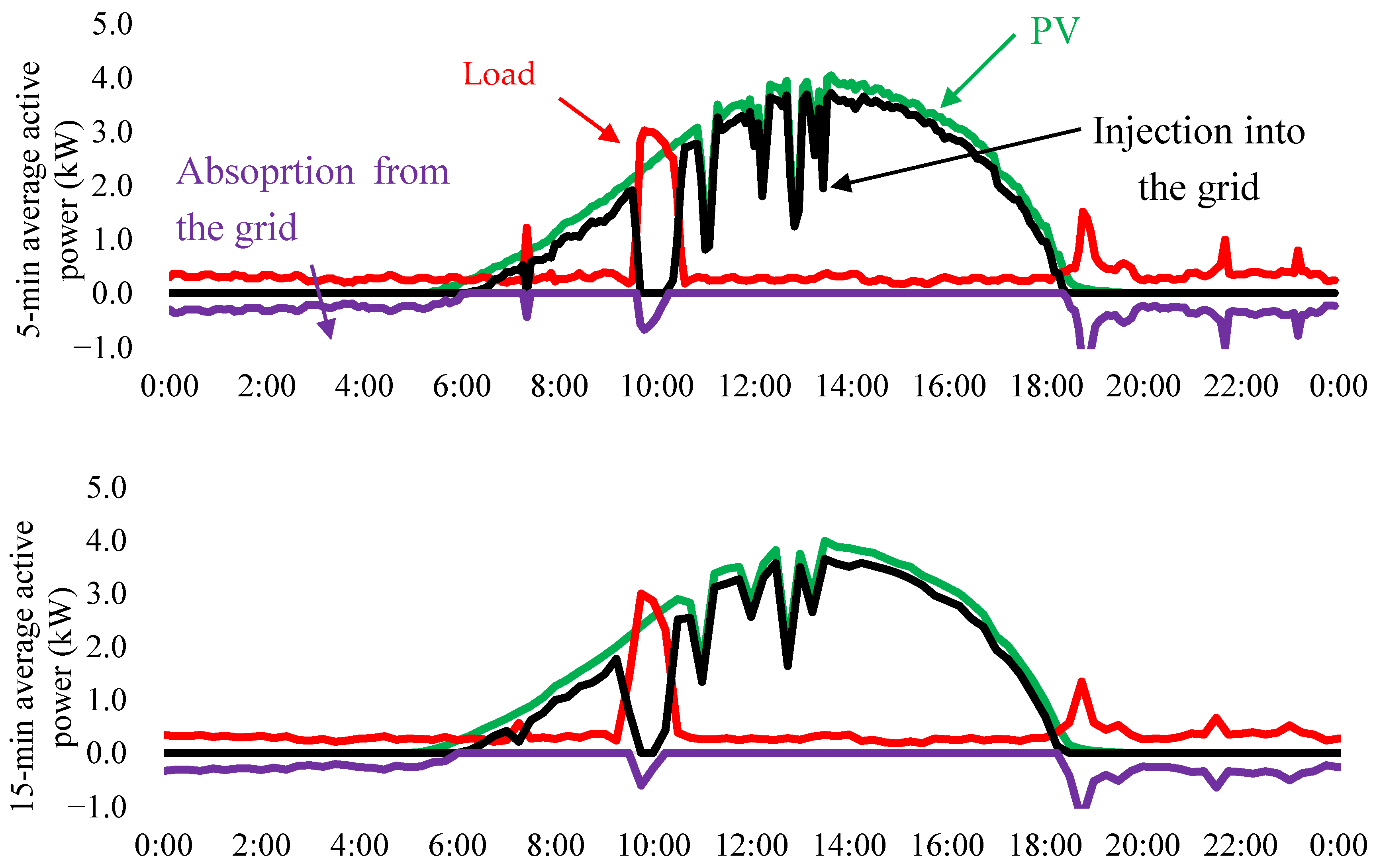
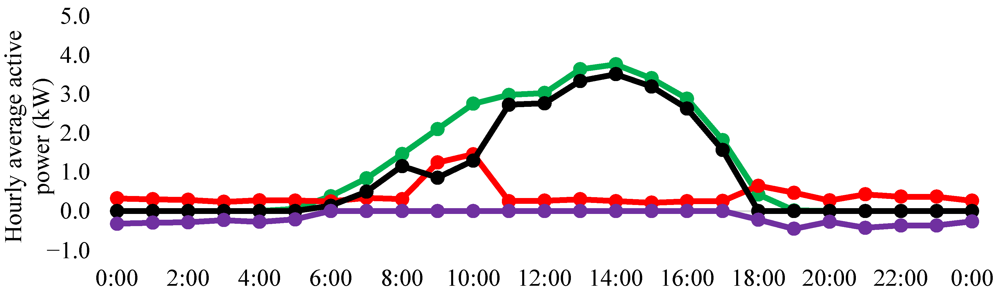
  39. Burgio, A.; Menniti, D.; Sorrentino, N.; Pinnarelli, A.; Leonowicz, Z. Influence and Impact of Data Averaging and Temporal Resolution on the Assessment of Energetic, Economic and Technical Issues of Hybrid Photovoltaic-Battery Systems. Energies 2020, 13, 354. [Google Scholar] [CrossRef] [Green Version]
  40. Beck, T.; Kondziella, H.; Huard, G.; Bruckner, T. Assessing the influence of the temporal resolution of electrical load and PV generation profiles on self-consumption and sizing of PV-battery systems. Appl. Energy 2016, 173, 331–342. [Google Scholar] [CrossRef]
  41. Sun, S.I.; Smith, B.D.; Wills, R.G.A.; Crossland, A.F. Effects of time resolution on finances and self-consumption when modeling domestic PV-battery systems. Energy Rep. 2020, 6, 157–165. [Google Scholar] [CrossRef]
  42. European Commission. Regulation 2017/2195 of 23 November 2017 Establishing a Guideline on Electricity Balancing C/2017/7774. Available online: http://data.europa.eu/eli/reg/2017/2195/oj (accessed on 20 January 2021).
  43. Ciocia, A.; Ahmad, J.; Chicco, G.; Di Leo, P.; Spertino, F. Optimal size of photovoltaic systems with storage for office and residential loads in the Italian net-billing scheme. In Proceedings of the 51st International Universities Power Engineering Conference (UPEC), Coimbra, Portugal, 6–9 September 2016; pp. 1–6. [Google Scholar]
  44. Schujman, S.B.; Mann, J.R.; Dufresne, G.; LaQue, L.M.; Rice, C.; Wax, J.; Metacarpa, D.J.; Haldar, P. Evaluation of protocols for temperature coefficient determination. In Proceedings of the 2015 IEEE 42nd Photovoltaic Specialist Conference (PVSC), New Orleans, LA, USA, 14–19 June 2015; pp. 1–4. [Google Scholar]
  45. Liu, S.; Dong, M. Quantitative research on impact of ambient temperature and module temperature on short-term photovoltaic power forecasting. In Proceedings of the 2016 International Conference on Smart Grid and Clean Energy Technologies (ICSGCE), Chengdu, China, 19–22 October 2016; pp. 262–266. [Google Scholar]
  46. National Renewable Energy Laboratory of U.S.A. Photovoltaic Degradation Rates—An Analytical Review. Available online: https://www.nrel.gov/docs/fy12osti/51664.pdf (accessed on 2 July 2020).
  47. Carullo, A.; Castellana, A.; Vallan, A.; Ciocia, A.; Spertino, F. In-field monitoring of eight photovoltaic plants: Degradation rate over seven years of continuous operation. Acta IMEKO 2018, 7, 75–81. [Google Scholar] [CrossRef]
  48. Spertino, F.; Ciocia, A.; Cocina, V.; Di Leo, P. Renewable sources with storage for cost-effective solutions to supply commercial loads. In Proceedings of the 2016 International Symposium on Power Electronics, Electrical Drives, Automation and Motion (SPEEDAM), Anacapri, Italy, 22–24 June 2016; pp. 242–247. [Google Scholar]
  49. Di Leo, P.; Spertino, F.; Fichera, S.; Malgaroli, G.; Ratclif, A. Improvement of Self-Sufficiency for an Innovative Nearly Zero Energy Building by Photovoltaic Generators. In Proceedings of the 2019 IEEE Milan PowerTech, Milan, Italy, 23–27 June 2019; pp. 1–6. [Google Scholar]
  50. A Closer Look at State of Charge (SOC) and State of Health (SOH) Estimation Techniques for Batteries. Available online: https://www.analog.com/media/en/technical-documentation/technical-articles/A-Closer-Look-at-State-Of-Charge-and-State-Health-Estimation-Techniques-....pdf (accessed on 15 January 2021).
  51. Laajimi, M.; Go, Y.I. Energy storage system design for large-scale solar PV in Malaysia: Technical and environmental assessments. J. Energ. Storage 2019, 26, 100984. [Google Scholar] [CrossRef]
  52. Zeh, A.; Müller, M.; Naumann, M.; Hesse, H.C.; Jossen, A.; Witzmann, R. Fundamentals of Using Battery Energy Storage Systems to Provide Primary Control Reserves in Germany. Batteries 2016, 2, 29. [Google Scholar] [CrossRef] [Green Version]
  53. Carullo, A.; Ciocia, A.; Di Leo, P.; Giordano, F.; Malgaroli, G.; Peraga, L.; Spertino, F.; Vallan, A. Comparison of correction methods of wind speed for performance evaluation of wind turbines. In Proceedings of the 24th IMEKO TC4 International Symposium and 22nd International Workshop on ADC and DAC Modelling and Testing, Palermo, Italy, 14–16 September 2020; pp. 291–296. [Google Scholar]
  54. Lin, C.; Hsieh, W.; Chen, C.; Hsu, C.; Ku, T. Optimization of Photovoltaic Penetration in Distribution Systems Considering Annual Duration Curve of Solar Irradiation. IEEE Trans. Power Syst. 2012, 27, 1090–1097. [Google Scholar] [CrossRef]
  55. U.S. Energy Information Administration. Levelized Cost and Levelized Avoided Cost of New Generation Resources in the Annual Energy Outlook. 2016. Available online: http://www.eia.gov/outlooks/aeo/pdf/electricity_generation.pdf (accessed on 20 January 2021).
  56. Rajput, P.; Malvoni, M.; Manoj Kumar, N.; Sastry, O.S.; Jayakumar, A. Operational Performance and Degradation Influenced Life Cycle Environmental–Economic Metrics of mc-Si, a-Si and HIT Photovoltaic Arrays in Hot Semi-arid Climates. Sustainability 2020, 12, 1075. [Google Scholar] [CrossRef] [Green Version]
  57. Spertino, F.; Ahmad, J.; Chicco, G.; Ciocia, A.; Di Leo, P. Matching between electric generation and load: Hybrid PV-wind system and tertiary-sector users. In Proceedings of the 2015 50th International Universities Power Engineering Conference (UPEC), Stoke on Trent, UK, 1–4 September 2015; pp. 1–6. [Google Scholar]
  58. Ullah, A.; Imran, H.; Maqsood, Z.; Zafar Butt, N. Investigation of optimal tilt angles and effects of soiling on PV energy production in Pakistan. Renew. Energy 2019, 139, 830–843. [Google Scholar] [CrossRef]
  59. Spertino, F.; Ahmad, J.; Ciocia, A.; Di Leo, P. How much is the advisable self-sufficiency of aggregated prosumers with photovoltaic-wind power and storage to avoid grid upgrades? In Proceedings of the 2017 IEEE Industry Applications Society Annual Meeting, Cincinnati, OH, USA, 1–4 October 2017; pp. 1–8. [Google Scholar]
  60. ElSayed, S.K.; Elattar, E.E. Hybrid Harris hawks optimization with sequential quadratic programming for optimal coordination of directional overcurrent relays incorporating distributed generation. Alex. Eng. J. 2021, 60, 2421–2433. [Google Scholar] [CrossRef]
  61. Euro-Mongolian Cooperation for Modernization of Engineering Education (EU MONG). Available online: http://eu-mong.eu/ (accessed on 28 May 2020).
  62. Tzanova, S. Work in Progress: Competence Building in Engineering Education in Mongolia. In Proceedings of the EDUCON 2020, Porto, Portugal, 27–30 April 2020; pp. 33–36. [Google Scholar]
  63. Gestore dei Servizi Energetici (GSE). Available online: https://www.gse.it/documenti_site/Documenti%20GSE/Rapporti%20statistici/Relazione_annuale_situazione_energetica_nazionale_dati_2018.pdf (accessed on 14 May 2020).
  64. Italian Law, DM 04/07/2019. Accesso agli Incentivi. Available online: https://www.gse.it/servizi-per-te/fonti-rinnovabili/fer-elettriche/incentivi-dm-04-07-2019 (accessed on 4 July 2020).
  65. Gestore dei Servizi Energetici (GSE). Available online: https://www.gse.it/servizi-per-te/fotovoltaico/scambio-sul-posto (accessed on 18 May 2020).
  66. GSE. Servizio di Scambio sul posto: Regole Tecniche. Available online: https://www.gse.it/documenti_site/Documenti%20GSE/Servizi%20per%20te/SCAMBIO%20SUL%20POSTO/Regole%20e%20procedure/Regole%20Tecniche%20Scambio%20sul%20Posto_2019.pdf. (accessed on 15 June 2020).
  67. ARERA. Valori del Corrispettivo Unitario di Scambio Forfetario per l’anno. 2019. Available online: https://www.arera.it/allegati/comunicati/CorrispettiviCUsf2019.pdf (accessed on 15 June 2020).
  68. Ciocia, A.; Di Leo, P.; Malgaroli, G.; Spertino, F. Subhour Simulation of a Microgrid of All-Electric nZEBs Based on Italian Market Rules. In Proceedings of the 2020 IEEE International Conference on Environment and Electrical Engineering and 2020 IEEE Industrial and Commercial Power Systems Europe (EEEIC/I&CPS Europe), Madrid, Spain, 9–12 June 2020; pp. 1–6. [Google Scholar] [CrossRef]
Figure 1. Generic example of PV generation and load profiles of a domestic user.
Energies 14 01591 g001
Figure 2. Scheme of the procedure used in the tool with indication of the inputs/outputs.
Energies 14 01591 g002
Figure 3. Comparison of power profiles with different time-steps: 5 min (top), 15 min (in the middle), and 1 h (bottom).
Energies 14 01591 g003aEnergies 14 01591 g003b
Figure 4. PV efficiency as function of irradiance and temperature (a) and DC/AC conversion efficiency (b).
Energies 14 01591 g004
Figure 5. Example of energy flows during a summer day.
Energies 14 01591 g005
Figure 6. Monthly electricity consumption of the analyzed residential user.
Energies 14 01591 g006
Figure 7. Load power profiles of a day in February and July.
Energies 14 01591 g007
Figure 8. Consumer and prosumer economic annual balance.
Energies 14 01591 g008
Figure 9. Self-sufficiency and IRR as functions of PV nominal power for different injection limits.
Energies 14 01591 g009
Figure 10. SC and SS as functions of PV nominal power with different injection limits.
Energies 14 01591 g010
Figure 11. Self-sufficiency and NET Present Value (NPV) as functions of PV nominal power with different injection limits.
Energies 14 01591 g011
Figure 12. Example of hourly energy profiles of the analyzed residential user during an autumn day.
Energies 14 01591 g012
Figure 13. Hourly energy profiles of Figure 11 with a curtailment in the grid injection I.L. = 1 kWh/h.
Energies 14 01591 g013
Figure 14. PV nominal power, BESS nominal energy, and maximum SS for different BESS costs.
Energies 14 01591 g014
Table 1. Energy quantities related to the example in Figure 3: daily balances.
Energy QuantitiesMeasurement UnitTime Step
5 min15 min1 h
ConsumptionkWh9.69.69.6
PV generationkWh29.629.629.6
Injection in the gridkWh24.224.123.7
Absorption from the gridkWh−4.3−4.2−3.8
Self-sufficiency-55.6%56.6%61.1%
Self-consumption-18.1%18.5%19.9%
Table 2. Energy quantities related to the example in Figure 3: yearly balances.
Energy QuantitiesMeasurement UnitTime Step
5 min15 min1 h
ConsumptionkWh670067006700
PV generationkWh571557155715
Injection in the gridkWh331832543102
Absorption from the gridkWh−4303−4238−4087
Self-sufficiency-35.8%36.7%39.0%
Self-consumption-41.9%43.1%45.7%
Table 3. Main results of the reference case.
Energy and Economic QuantitiesMaximization of Self-SufficiencyMaximization of NPV
No I.L.I.L. =
2 kWh/h
I.L. =
0 kWh/h
No I.L.I.L. =
2 kWh/h
I.L. =
0 kWh/h
PV
nominal power
13 kW10 kW5 kW6 kW6 kW4 kW
SS49%48%41%43%43%38%
SC21%40%100%40%45%100%
IRR6.4%6.3%6.5%11.2%10.5%8.0%
NPVEUR 7423EUR 5657EUR 2996EUR 9594EUR 8663EUR 3571
Table 4. Main results of the case with PV plant coupled to BESS.
Energy and Economic QuantitiesMaximization of Self-Sufficiency
No I.L.I.L. =
3 kWh/h
I.L. =
2 kWh/h
I.L. =
1 kWh/h
I.L. =
0 kWh/h
PV nominal power7 kW7 kW7 kW6 kW4 kW
BESS nominal energy6 kWh6 kWh5 kWh4 kWh4 kWh
SS65%65%62%58%52%
SC51%54%59%71%98%
IRR6.4%6.1%6.4%6.4%6.2%
NPVEUR 4364EUR 4028EUR 4278EUR 3654EUR 2367
Publisher’s Note: MDPI stays neutral with regard to jurisdictional claims in published maps and institutional affiliations.

