1. Introduction
Favorable economics of investment in rooftop photovoltaics (PV) in many jurisdictions around the world has increased self-generation of PV electricity to supplement electricity purchased from the power grid [
1,
2]. This trend has implications for utilities’ planning and operation, as increased self-generation from PV can have technical impacts on the grid as well as reduce utilities’ revenue from electricity sale [
3,
4]. For this reason, countries or regions with high penetration of rooftop PV systems have developed advanced tools for forecasting how rooftop PV penetration is likely to evolve over the short- and long-term [
5,
6,
7,
8,
9,
10,
11].
As rooftop PV markets are just beginning to grow in many developing countries, rooftop PV penetration is presently low and has only minimal impacts on the power system. Yet, forecasts of rooftop PV penetration are still useful. Such forecasts can inform policy to ensure equitable access to PV, as well as stimulate innovative business models for targeted consumer groups in different regions. State-of-the-art tools for PV forecasting are related to modeling the adoption of PV and the modeling methods are various and come from research institutes, industry experts and utility companies. Research institutes and industry experts often develop sophisticated and comprehensive tools such as bottom-up customer adoption while utility companies prefer uncomplicated methods such as extrapolating from historical data [
12]. Generally, comprehensive tools rely on data sets that are largely unavailable in developing countries. Additionally, the historical data of PV capacity for self-consumption are available only a few years as PV deployment is at the early stage.
To address this challenge, we developed a simplified analytical tool for assessing rooftop PV “hotspots”—that is, geographical areas where a large number of new investments into rooftop PV investments are likely to occur and impose a high financial impact on the utility. The tool combines the assessment of two indicators, (1) a financial indicator (represented by the capital-to-expenditure ratio and the capital-to-bill ratio) and (2) a technical indicator (represented by the PV-to-load ratio). Combined assessment of these two indicators enables users to compare the relative level of rooftop PV adoption across regions.
Despite its simplicity, the tool presented in this paper has several advantages compared to the state-of-the-art PV forecasting tools. First, it relies on relatively few data sets that are more readily available in developing countries. This means the tool can be easily adapted to be used in other countries. Second, it is transparent and allows the users to clearly understand the relationship between the financial and technical indicators. Third, the tool treats the electricity consumer as a rational economic agent who maximizes his net benefit, in this case the Net Present Value (NPV) of rooftop PV installation. By solving for the optimal PV size that maximizes the NPV under different compensation mechanisms, the tool can provide an upper bound of the suitable PV compensation rate. However, several limitations of this tool are also acknowledged. Therefore, this tool can be deployed as a quick first screener for the potential PV hotspots. Once the market becomes more mature and data become more available, stakeholders can utilize the advanced state-of-the-art methods for a more detailed forecast.
Lastly, we demonstrate the use of this tool for the case of Thailand. Customer economics of rooftop PV adoption under two compensation mechanisms—self-consumption and net billing—are analyzed for different customer groups in different regions. Then, the potential rooftop PV hotspots are identified for the early and late stage. The results from the tool are helpful for policymakers or businesses seeking to design regionally tailored programs to stimulate rooftop PV adoption as discussed in the section of policy implications.
2. Literature Review
2.1. Forecasting Rooftop PV Deployment
There are various approaches to model PV expansion as the PV adoption is related to technology adoption where various theories and models of technology diffusion are deployed, such as diffusion theories, user acceptance theories, decision making theories, personality theories, and organization structure theories [
13]. For solar PV, modelling on the expansion of decentralized PV can be divided into three main families: economic regression, diffusion theories, and behavior of individual adoption [
14].
Economic regression analysis can be used to determine the relation between the rates of expansion and the macro-economic factors. For instance, a diffusion model using the logistic growth theory is used to predict the diffusion of renewable electricity in South Korea [
15]. In [
16], regression and correlational analysis are conducted to investigate the trends in rooftop solar adoption with socioeconomic, health and environmental indicators in California. Authors of [
17] combine different regression models to project PV installations for 1–5 years ahead at a subnational level. In [
11], the potential areas where rooftop PV systems are likely to be installed in Indian cities are estimated by using a regression model.
Another family of studies on PV adoption focuses on theories of diffusion. A large number of studies deploy the Bass diffusion model to estimate the solar PV market [
5,
6,
7,
8,
9,
10]. For instance, the Bass model is deployed to forecast the rooftop PV adoption as a part of the Distributed Generation Market Demand Model (dGen) developed by National Renewable Energy Laboratory (NREL) and the National Energy Modeling System constructed by Energy Information Administration [
8]. Other diffusion theories, such as the theory of disruptive innovation and the prospect theory, are applied to forecast the solar PV adoption [
18,
19].
The behavior of individual adoption is usually modeled by agent-based modeling approaches [
20,
21]. An integration of agent-based modeling with other approaches can be performed [
22,
23,
24]. For instance, in the dGen model [
23], customer decision making in PV adoption is modeled by an agent-based approach. The dGen model employs cash-flow analysis coupled with projections of market growth rates and overall market potential.
Selecting models of PV adoption depends on the objectives of studies and data availability. The larger scale of analysis with the inclusion of the economic and social perspectives, the more complexity of modelling and the greater data requirement. For instance, the economic regression analysis and Bass model need historical data at least five years to analyze the relation of parameters. The agent-based model demands individual data such as factors where customers use to decide in installing a PV system. Such individual data can be acquired through a survey where is usually required more resources.
Models for forecasting rooftop PV deployment help users understand the extent to which rooftop PV is likely to affect net demand for grid electricity. This understanding helps utilities plan for future capital and operating costs, ensure resource adequacy, and estimate possible revenue shortfalls. However, as an adoption of rooftop PV is increasing, collecting data on capacity and demographic data related to such rooftop PV adoption is difficult in developing countries.
The simplified model presented in this paper departs from the previous works in several respects. First, our approach identifies PV array sizes that maximize customer benefits to assess the maximum impacts of solar PV. This likely represents a conservative, upper-bound estimate of solar PV impacts, as there is not always suitable rooftop space available to accommodate the optimal array size. (Note that array size is constrained by a maximum allowable size for each customer class, as described in the section providing details of the optimization algorithm). Second, our model takes a static, rather than dynamic, approach to assess rooftop PV hotspots to reduce the data requirement. Third, our model examines the unconstrained maximization problem where a representative customer chooses a PV size that maximizes his or her NPV. The result provides the maximum PV penetration relative to load for different customer classes. As our model does not make assumptions about technology-adoption behavior, our results can be interpreted either as a “snapshot” of rooftop PV hotspots in the early stage when there is just one representative customer in all regions, or as the equilibrium landscape of rooftop PV hotspots in the long term, when all financial constraints are removed. Our model is simple, transparent, and relies on a minimum number of data sets while providing a geographically comparative analysis that can inform policymaking and business decisions. These characteristics are essential for stakeholders in developing countries, where rooftop PV markets are just beginning to take shape.
2.2. Factors of PV Adoption
Factors or predictors to decide on PV adoption are various [
12,
25,
26,
27]. Multiple models exist to forecast how these factors will combine to affect rooftop PV deployment. Basically, these factors can be classified into four main groups: PV economics, public policies, customer preferences, and macro factors according to [
12].
First, customer economics of rooftop PV are a key factor determining whether a customer chooses to adopt a rooftop PV system [
27,
28,
29,
30]. The customer economics of rooftop PV Customer benefits can be measured by financial indicators such as NPV, internal rate of return (IRR), payback period, and levelized cost of electricity (LCOE) [
28,
29,
31]. Many factors, such as PV installation costs, PV system performance, government policies, electricity prices, and new business models, can affect the economics of rooftop PV.
Second, public policies include government programs (i.e., tax incentives, subsidies, feed-in-tariff, self-consumption, net metering, net billing, etc.) [
14,
29,
31] and other form of policy support, such as renewable portfolio standards and climate change mitigation policies [
12,
32,
33]. Public policies have major influences on the solar PV adoption, especially in nascent markets. Additionally, availability of financing options is linked to regulations allowed in those countries [
34,
35,
36].
Third, decision making of customer to adopt solar PV is directly linked to the PV adoption rate. Examples of factors affecting customer decision are customer access to trustworthy information [
37], peer effects [
38,
39,
40], environmental concern [
41,
42], and the customer’s socioeconomic characteristics [
43,
44,
45]. For a residential customer, income has been the most frequently used to predict the PV adoption [
26]. Early adopters of rooftop PV systems tend to be high-income customers [
44,
46,
47].
Lastly, macro-economic factors, such as economic growth, load growth, oil and gas prices, and interest rates, also drive the adoption of PV and renewable energy [
7,
14,
15,
48,
49,
50,
51].
For this work, the factors of PV economics, PV policies, and customer preferences are considered since the analysis aims to help a utility company to identify the potential areas that could have comparatively high investment of solar PV based on the existing data.
3. Methodology and Data
Rooftop PV “hotspots” are defined as the geographical areas where abundant new rooftop PV investments are likely to occur. The hotspots are classified based on potential impacts on utilities and the likely timing of rooftop PV adoption. With respect to the former, areas exhibiting a favorable load profile, high irradiation levels, and suitable roofs will incentivize customers to invest in large PV systems (relative to a customer’s electricity demand) under a given compensation mechanism. This results in a high PV-to-load ratio and hence a high impact on the electric utility serving that area. Second, an area with wealthy customers (both residential and industrial) is likely to see early investments in rooftop PV systems if the investment yields favorable economic returns. (Poorer customers may not be able to finance the initial capital demands of even favorable investments).
The analysis is performed in two steps. First, the “optimal” PV size that maximizes the NPV of various customer classes in different provinces in Thailand is solved. The customer classes are considered according to the classes of retail electricity customers in Thailand: Residential (Res), Small General Service (SGS), Medium General Service (MGS), and Large General Service (LGS). Descriptions of these customer classes and tariff structure are in the
Appendix A.
Second, the optimal PV size is converted to the associated PV-to-load ratio. The ratio indicates the potential financial impact to the utility in the area [
52]. The PV-to-load ratio is then overlay with regional socioeconomic variables such as household income (for residential customers) or the level of industrial activity (for commercial and industrial customers). These socioeconomic variables serve as proxies for a customer’s wealth and for how easy it is to invest in the optimal rooftop PV in different regions. Investments in the rooftop PV are assumed to be made in 100% cash, as there are presently limited financing options in Thailand’s nascent rooftop PV market. As financing options expand and investment becomes easier, the likelihood of PV adoption in Thailand will increase.
It should be noted that although this paper illustrates the application at a provincial level, the level of aggregation under this framework is rather flexible. In particular, the financial and technical indicators proposed by this framework can be constructed based on finer geographical level as long as credible data on PV capacity factor, load profile, and other socio-economic indicators are available. In fact, the finer the geographical grid, the more precise the impact identified.
3.1. Solving for the Optimal Investment
In this study, an optimization objective is to maximize the NPV of PV investment as:
where
i represents the discount rate for each customer group considered and
k represents the PV size. The details of the financial and technical assumptions are provided in
Section 3.4 and in the
Appendix A.
A customer’s bill savings in each period (year) will result from two PV output parts. The first is the self-consumed part, which occurs when PV output (depending on the PV size and weather data) directly offsets a customer’s instantaneous load and thus the customer’s electricity bill. In other words, the self-consumed part is calculated from a subtraction between the hourly PV output and load profile. The second is the excess generation part, which is the PV output that exceeds the instantaneous load in each one-hour interval. Under some PV compensation policies described below, the excess generation can be sold back to the electricity grid in exchange for monetary credits.
Given the objective function, the optimal PV size that maximizes the NPV is solved by building a simulation tool based on the System Advisory Model (SAM) from the NREL. The SAM module simulates the PV output and computes NPV under various parameters [
53,
54]. The simulation tool varies the PV system size and calls SAM to search for the highest NPV for each customer class, location, and compensation mechanism. Once the optimal PV sizes are obtained, LCOE, IRR, and payback period are determined to quantify customer economics. The details of optimization algorithm and economic measures are in the
Appendix B and
Appendix C.
It should be noted that in determining the optimal PV size, the algorithm was done in iteration within the range of possible PV system sizes based on the observed typical PV sizing. The algorithm is not complicated, and it does not consume time to solve for one case. However, it was time-consuming to solve for all customer classes and provinces. In addition, the optimal value can converge to zero, infinity, or a non-zero finite value. If the optimal value goes to zero, it means that the consumer should not invest in the PV system at all. If the optimal value goes to infinity, it means the consumer should increase the size of the PV system to the largest possible. If the optimal value goes to a non-zero finite number, it means the customer should install a PV system of that size.
3.2. Determining the Investment Hotspots
The rooftop PV hotspots are defined by using two indicators: (1) the PV-to-load ratio and (2) the capital-to-wealth ratio. Rooftop PV hotspots are geographical areas with high PV-to-load ratios and low capital-to-wealth ratios, as discussed below. The two indicators are determined for each customer class, location, and compensation mechanism.
- (1)
The PV-to-load ratio is the ratio between the total PV output (from the “optimal” PV system size) and the total electricity demand in a year for a given customer, location, and compensation mechanism. In other words:
Note that this PV-to-load ratio measures the maximum installation size likely to be adopted by a representative customer when all the financial constraints are removed. A higher PV-to-load ratio implies that the customer of that particular group in that particular geographical area will likely adopt a larger PV system size compared to the existing load.
From a utility’s perspective, a utility in an area with a high optimal PV-to-load ratio will likely face a higher maximum financial impact due to reduced electricity purchases from the grid relative to a scenario in which rooftop PV is not available. Utility revenue reduction caused by rooftop PV is heightened when net metering is combined with a rate structure that is primarily based on volumetric charges [
4,
55].
One caveat is that the PV-to-load ratio can only suggest the level of impact relative to the status quo of no PV penetration within the same area. It cannot be used to compare the absolute level of PV penetration across areas. For example, a small province can have a high optimal PV-to-load ratio, but the absolute level of PV penetration—and hence the net financial impact on the utility serving the area—will remain small due to the small size of the population. Forecasting the absolute level of penetration and utility’s financial impact requires additional assumptions regarding consumer income distribution as well as the technology-adoption behavior, both of which are beyond the scope of the paper.
- (2)
The capital-to-wealth ratio is the ratio between the capital cost for an optimally sized PV system and a customer’s wealth. This indicator measures how easy it is for an average customer to finance the optimally sized PV system.
For residential and SGS customers, monthly expenditure per capita—averaged over all households in each province—is used as a proxy for wealth. The same proxy for residential and SGS customers’ wealth is used since they represent similar decision-making units (i.e., SGS customers are residential customers who run their small business locally). In essence, the “capital-to-expenditure” ratio for these customer classes asks how many months of expenditure it takes for a customer to be able to invest in the optimally sized PV. The lower the capital-to-expenditure ratio, the easier it is to finance such investment.
It should be noted that an ideal proxy for the ability to finance an optimally sized PV system would be the customer’s saving (income minus expenditures). However, data on monthly household income in Thailand is often underreported. Monthly expenditure per capita, on the other hand, reflects real behavior and is much less likely to be underreported. Therefore, monthly expenditure per capita is used rather than saving as a proxy for a household’s real wealth. The per-capita definition also implicitly accounts for the different average household sizes in different locations.
Due to data limitations, the financial constraint indicator for MGS and LGS customers is the capital-to-(electricity) bill ratio instead of the capital-to-(household) expenditure ratio used for residential and SGS customers. The median monthly electricity bill is used as a proxy for business performance. The higher the electricity bill, the larger and more active a business is. This “capital-to-bill ratio” has a different denominator than the capital-to-expenditure ratio used for residential and SGS customers; therefore, these ratios are not directly comparable. It should be noted that the monthly electricity bill is not a perfect measure for the real business activity since some types of business are by nature more energy-intensive than others. However, the ability to pay for the electricity bill does reflect the financial capability of the customer (regardless of the business type) and the ability to finance a rooftop PV.
Figure 1 illustrates the concept of the rooftop PV hotspot. An area with a high PV-to-load ratio and a low capital-to-wealth ratio is likely to be a rooftop PV hotspot in the early stage of PV market development (dark grey area). This is because the representative customer in this area already faces a lower financial constraint (low capital-to-wealth ratio) and can afford to invest up to the large optimal rooftop PV size (high PV-to-load ratio). The light grey area indicates the area where the customer can afford to invest in the optimal rooftop PV size (low capital-to-wealth ratio), but the optimal PV sizes may not be as high as in the dark grey area (low PV-to-load ratio). By contrast, customers in the top area in
Figure 1 have higher capital-to-wealth ratios and will likely be late adopters of rooftop PV.
To determine the investment hotspots, the procedure can be summarized as shown in
Figure 2.
3.3. Compensation Policies
Two PV compensation mechanisms are considered in this study: self-consumption and net billing, both of which assume that output from rooftop PV first serves the load. The major difference between the two policies is how the excess PV generation is compensated.
First, the self-consumption policy allows excess PV output to be sent back to the grid. However, this excess output will be valued at zero THB (Thai baht). Examining the self-consumption compensation mechanism is useful for the following reasons. First, self-consumption requires minimal governmental support. Second, self-consumption does not depend on the existence of a third-party consumer. Finally, self-consumption of rooftop PV is already permitted in Thailand.
Second, the net billing policy allows excess PV output to be sent back to the grid and compensated at a non-zero “buyback rate.” The compensation is first used to offset the customer’s electricity bill at the end of the month. Any remaining monetary credits can be “rolled over” to offset future bills for up to 12 months. The net-billing compensation mechanism is chosen for the following reasons. First, net billing is flexible enough to encompass other well-known compensation mechanisms (e.g., net metering). Second, net billing is largely displacing net metering as the compensation mechanism of choice. Net billing has been the most common compensation mechanism adopted in the U.S. states that have opted for something other than net metering [
56]. Net billing is being considered to replace existing compensation mechanisms in the Philippines [
57] and has recently been approved as a new compensation mechanism for rooftop PV in Thailand [
58].
In many jurisdictions employing net billing, the buyback rate has fallen to a level lower than the retail rate as declining costs of rooftop PV have made it less necessary to provide strong financial incentives for consumers to invest in solar. This study includes a sensitivity analysis of buyback rate by considering three buyback rate levels: 1 THB/kWh (0.029 USD/kWh), 2 THB/kWh (0.058 USD/kWh), and 3 THB/kWh (0.086 USD/kWh). As governmental stakeholders including policymakers, utilities, and regulators prefer a buyback rate lower than the retail rate [
28], the highest buyback rate considered in our sensitivity analysis is approximately the average wholesale time-of-use (TOU) electricity price at the lowest voltage level.
3.4. Data
3.4.1. Data for Calculating the Optimal PV Size
Data used to perform the rooftop PV economic analysis comes from two sources. The load profile data come from the Load Profile Study conducted in 2015 by the Provincial Electricity Authority (PEA). The PEA is the largest distribution utility in Thailand. It serves retail customers throughout Thailand except in the Bangkok Metropolitan area. The load profile data for each customer type consists of 12-month hourly power in four different geographical regions: North (N), the Northeast, Central (C), and South (S) Thailand (
Figure 3). There are hence four different 8760-hour load profiles for each customer type as shown in the
Appendix A. The hourly weather data needed to simulate rooftop PV output were obtained from White Box Technologies, which provides “typical year” weather profiles for 56 weather stations in Thailand [
59].
Figure 4 shows the average capacity factor for a modeled rooftop PV system in provinces where weather data is available. The figure reveals that PV productivity is highest in the northern and northeastern provinces and lowest in the southern provinces.
Table 1 shows the average capacity factor across the four regions.
The PV system optimization is conducted at the provincial level—the finest geographic scale at which sufficient data are available. This means that for each customer type and compensation policy, 56 optimal PV values are generated associated with 56 provinces.
3.4.2. Technical and Financial Assumptions for Calculating the Optimal PV Size
Technical details of the system-design and financial assumptions used as inputs into SAM are summarized in the
Appendix A. Electricity rates are those published by the PEA. The installation costs of solar PV systems are based on the market price survey from EPC and other financial assumptions to reflect the conditions of Thailand’s solar PV market between the months of August and December 2016.
3.4.3. Data on Regional Economic Activity
The regional socioeconomic data in this study come from two different sources. The province-level average household monthly expenditures per capita (used as a proxy for residential and SGS customers’ wealth) in 2015 come from Thailand’s National Statistical Office [
60]. The province-level median per-meter electricity bills (used as a proxy for MGS and LGS customers’ economic activity) come from the PEA.
Figure 5 shows the socioeconomic measures for each customer group studied. On average, residential and SGS customers in the Southern and Eastern provinces have the highest expenditures per capita (wealth) and thus should face the lowest financial constraints for rooftop PV investment. A similar pattern of MGS customers is observed—the median bill payment (economic activity) is highest in the Southern and Eastern provinces. On the other hand, LGS customers exhibit the highest bill payment in the Northern provinces and Nakhon Ratchasima (a province in Northeastern Thailand).
The geographical distributions of median electricity bill payment for MGS and LGS customers in
Figure 5 are consistent with the major economic activities in each region. Specifically, the MGS’ median electricity consumption is highest in the South, which is driven mainly by the tourism industry. The LGS’ median electricity consumption, on the other hand, is highest in the North and Eastern provinces due to manufacturing activities [
61].
4. Results and Discussions
This section discusses the resulting optimal PV investment and the potential PV hotspots for each customer group. As stated above, there are 56 optimal PV values associated with 56 provinces for each customer class and compensation scheme. To simplify the discussion, the averaged values of the results across all provinces within the same geographical region are presented. Detailed results on LCOEs, IRRs, and payback periods for each customer class are shown in the
Appendix C.
4.1. Optimal PV Investment
When the buyback rate for excess generation is 3 THB/kWh, the optimal PV size for all customer classes hits an upper optimization bound. This suggests that the gain from selling the excess generation exceeds the additional cost of investment. It also implies that the buyback rate that encourages self-consumption for all customers should be below 3 THB/kWh. For the rest of discussion, the optimization results when the buyback rate is 3 THB/kWh are omitted, since these do not reflect reasonable optimal values but rather values at the optimization bound.
4.1.1. Residential and Small General Service Customers
For residential customers, a higher buyback rate results in a larger optimal PV system size as well as a higher optimal NPV in each region (
Figure 6). For buyback rates at 2 THB/kWh and below, PV investment offers the highest NPV in the Northeastern region followed by the Central, Southern, and Northern regions, respectively. The average NPV in the North is lower than the average NPV in other regions mainly because of the amount of electricity consumption and the shape of the load profile.
According to the load profile (in the
Appendix A), residential customers in the North consume the least electricity and exhibit a very low loads during the day and high loads in the morning and evening compared to other regions. Therefore, most electricity generated from PV systems in the North will be exported to the grid and compensated at the low values. This suggests that electricity-consumption level and load-profile shape are key factors in determining optimal PV size.
Similar trends are observed for average optimal PV system size and NPV for residential customers with a TOU rate (
Figure 7). When a buyback rate is higher, an optimal PV system size and NPV are also higher. However, when compared to residential customers with a block rate, the TOU customers obtain slightly higher NPV despite the same average optimal PV system size. This observation implies that the tariff structures (block rate versus TOU rate) have some impacts on PV investments.
Like residential customers, SGS customers in each region are induced to install larger PV systems as the buyback rate for excess generation increases. Under the block rate with a buyback rate of 2 THB/kWh, average optimal PV sizes across all regions are approximately the same but the average NPV varies. The average NPV is highest in the Northeastern region followed by the Northern, Central, and Southern regions, respectively (
Figure 8). A buyback rate of 2 THB/kWh likely induces all SGS customers to install larger PV systems to gain benefits from surplus PV generation. It is likely that surplus PV generation depends heavily on geographical capacity factor, as average consumption during the day for SGS customers does not vary significantly by region. Variation in capacity factor leads to the average NPV ranking stated above.
If the buyback rate is below 2 THB/kWh, though, average NPVs stay the same across all regions while average optimal PV sizes are larger in regions with the lower capacity factors. This is likely because a lower buyback rate results in the geographical capacity factor assuming more weight in the determination of optimal PV size.
Similar patterns for average optimal PV size are observed for SGS customers under a TOU rate as (
Figure 9). SGS customers in each region are induced to install larger PV systems as a buyback rate is higher. However, SGS customers under a TOU rate install PV systems of approximately the same size as the SGS customers under a block rate but obtain a higher NPV. This implies that tariff structures impact PV investments.
Based on the optimal PV sizes, the average LCOE range across all regions (
Table 2) is 0.096–0.112 USD/kWh for both customer classes. These LCOEs are higher than the lowest block rate (0.0929 USD/kWh) and TOU rate during off-peak period (0.0754 USD/kWh). This implies that, given this paper’s set of assumptions, grid parity does not occur even if customers install the optimal PV size. The average electricity demand met by solar across all regions is 24.99–30.03% for residential customers and 29.53–40.86% for SGS customers. For the self-consumption ratios (
Table 3), based on the optional PV sizes, the average self-consumption range across all regions and schemes is 41.33–61.45% for residential customers and 41.37–58.70% for SGS customers. The net-billing scheme leads to lower self-consumption ratios because customers install larger PV systems when receiving compensation for excess PV electricity.
4.1.2. Medium General Service and Large General Service Customers
The optimal PV size for MGS customers increases with the buyback rate (
Figure 10). Given that the MGS load profiles are similar across regions (in the
Appendix A), the major determinants of optimal PV size are buyback rate and geographical capacity factor. In the regions with a relatively good capacity factor (North, Northeast, and Central), the optimal PV size at a buyback rate of 2 THB/kWh is significantly higher than the optimal PV size at 1 THB/kWh. This suggests that the benefit from excess electricity sales starts to exceed the cost of investment at a buyback rate of 2 THB/kWh. On the other hand, optimal PV size at a buyback rate of 1 THB/kWh is more similar to the size under a self-consumption scheme in all regions, which implies a limited return on excess electricity compared to the 2 THB/kWh buyback rate case.
The Northern and Northeastern regions feature the highest average NPV for MGS customers, followed by the Central and Southern regions, respectively. Geographical capacity factor is likely a key determinant of NPV for MGS customers. In addition, benefits for MG customers increase even more since the shape of generated PV profile matches the shape of the load profile. This means that PV helps meet peak demand and hence reduces demand charges.
The optimal PV size for LGS customers increases as the buyback rate increases (
Figure 11). The major determinants of optimal PV size for LGS customers are buyback rate and geographical capacity factor. The Central region offers the highest NPV, followed by the Northeastern, Southern, and Northern regions, respectively. Although the average optimal PV size in the Central region is larger than the average optimal size in the Northeastern region, the NPV in the Central region is higher than the NPV in the Northeastern region since customers in the Central region benefit more from reduction of consumption and peak demand. Average NPV is lowest in the Northern region, mainly because of the low amount of electricity consumption that generally occurs in Northern provinces.
Table 4 reports LCOEs associated with the optimal PV size by region for MGS and LGS customers. These LCOEs are higher than the off-peak rate (0.07514 USD/kWh) and peak rate (0.1203 USD/kWh). This implies that, given the set of assumptions used by this paper, grid parity does not occur even if customers install the optimal PV size. The average electricity demand met by solar across all regions is 32.95–44.22% for MGS customers and 31.22–36.66% for LGS customers. For the self-consumption ratios (
Table 5), based on the optional PV sizes, the average self-consumption range across all regions and schemes is 53.97–73.13% for MGS customers and 47.42–69.36% for LGS customers. The self-consumption ratios under the net-billing scheme are lower than those under self-consumption scheme for both customer classes.
The results of optimal PV investment across geographical regions suggest that different load profiles and support schemes can lead to different self-consumption levels. For residential and SGS customers, the average self-consumption range is 55.50–61.45% for the self-consumption scheme and 41.33–54.42% for the net-billing scheme. For MGS and LGS customers, the average self-consumption range is 63.15–73.13% for the self-consumption scheme and 47.42–71.64% for the net-billing scheme. The ratios for self-consumption in this study may be too high for residential customers while too low for the SGS, MGS, and LGS customers according to the self-consumption ratios in [
62]. The self-consumption share of residential customers should be low since no one is likely to be home during the day, so the electricity generated from a PV system is not used at the site. On the other hand, the load profiles of SGS, MGS, and LGS have higher demand during the day, which is aligned with the profile of PV production. Therefore, the self-consumption share could be up to 80% [
62].
For the studies related to self-consumption of solar PV in Thailand, the self-consumption level is rarely mentioned [
28,
29,
63]. In [
63], the self-consumption level for residential is 84.25% for the PV size of 5 kW. For [
28,
29], there are not data on self-consumption ratios, but the PV-to-load ratios are mentioned. In [
29] with the closest assumptions of the buyback rate for net-billing, but the different methods for setting PV sizes, the authors suggested that the appropriate PV systems should give the PV-to-load ratios approximately not greater than 30% for residential and SGS customers, and not greater than 40–50% for MGS and LGS customers. This is different from this study where the PV-to-load ratios for the net billing scheme are far higher (56.27–103.28% for residential and SGS customers and 48.74–85.84% for MGS and LGS customers).
4.2. Investment Hotspots
For simplicity, the investment hotspot results under the net billing consumption scheme with a buyback rate of 1 THB/kWh are presented. The results under other compensation policies are similar in relative terms.
4.2.1. Residential Customers
Figure 12 shows the relationship between the optimal PV-to-load ratio and the capital-to-expenditure ratio for residential customers in each province. Panel A shows the scatterplot of the relationship by province and Panel B displays the outcome variables by geographical location. Higher PV-to-load ratio indicates higher maximum financial impacts likely felt by the utility serving a region. A higher capital-to-expenditure ratio indicates that it is harder to self-finance such investment.
Three key insights emerge. First, homeowners in the Northeastern provinces are likely to be the late adopters of rooftop PV due to high financial constraints. The capital costs of rooftop PV in Northeastern provinces can be as high as 35× the average household monthly expenditure per capita. If optimal PV investments materialized, the PV-to-load ratios and the financial impact on utilities in this region will be higher relative to the case with no PV penetration. Second, the early residential rooftop PV adopters will likely be homeowners in the Northern provinces, which are characterized by an average PV-to-load ratio of 50%. Finally, the Central and Southern regions yield inconclusive results since there is less clustering of the capital-to-expenditure ratios compared to the other two regions.
Among residential customers, the early rooftop PV hotspots will be concentrated in the Northern region. The maximum financial impacts of these early hotspots on utilities will be moderate. Hotspots will likely emerge in the Northeastern region later on, with larger financial impacts on utilities.
4.2.2. Small General Service Customers
The relationship between the optimal PV-to-load ratio and the capital-to-expenditure ratio for SGS customers is shown in
Figure 13. The major difference between the SGS and the residential customer is that the SGS customers exhibit higher loads during the day.
For SGS customers, there is little clustering of capital-to-expenditure ratios by region. In other words, no region stands out as considerably better than others in terms of PV affordability. Regional trends do emerge for PV-to-load ratios. If financial constraints are removed and optimal PV investments are realized, the Northern region exhibits the highest PV-to-load ratios and the largest utility impacts relative to the case with no PV penetration.
In short, there are no obvious early rooftop PV hotspots for SGS customers. As the rooftop PV market matures, hotspots are likely to emerge in the Northern region, with large impacts on utilities.
4.2.3. Medium General Service Customers
The relationship between the optimal PV-to-load ratio and the capital-to-bill ratio for MGS customers is shown in
Figure 14. Similar to SGS customers, there is little clustering of capital-to-bill ratios by region for MGS customers. In other words, no region stands out as considerably better than others in terms of PV affordability. Regional trends do emerge for PV-to-load ratios. If financial constraints are removed and optimal PV investments are realized, the Northern and Northeastern regions exhibit the highest PV-to-load ratios and the largest utility impacts relative to the case with no PV penetration.
For MGS customers, there are no obvious early rooftop PV hotspots for MGS customers. As the rooftop PV market matures, hotspots are likely to emerge in the Northern and Northeastern regions, with large impacts on utilities.
4.2.4. Large General Service Customers
Figure 15 shows the relationship between the optimal PV-to-load ratio and the capital-to-expenditure ratio for LGS customers. Unlike the SGS and MGS customers, there is a clear clustering of the Northern provinces around the low capital-to-bill and high PV-to-load region of the scatterplot. This suggests that provinces in the Northern region will be early rooftop PV hotspots for LGS customers, imposing large financial impacts on utilities. The maximum penetration of rooftop PV for LGS customers is observed in the Northern region could be as high as 65% of load.
4.3. Policy Implications
Table 6 summarizes the findings of the previous sections by listing the regions where optimal PV investment can occur more easily (“early hotspots”) and where optimal PV investment faces higher financial constraint (“late hotspots”), as well as the penetration level (PV-to-load ratio) if such investment materializes. The Northern and Northeastern regions are clearly marked as the potential hotspots where the utility’s impact will be realized early or strongly or both.
This study reveals substantial variation in the optimal PV-to-load ratio (i.e., PV penetration) across four regions in Thailand. This variation results from regional heterogeneity in the load profiles and PV capacity factors. Yet, the optimal level of penetration may not materialize initially due to financial constraints faced by customers. Indeed, our analysis also reveals substantial variation in financial constraints (as measured by the capital-to-expenditure ratio) faced by different customer types in different regions.
These results can inform policy to ensure that customers in all parts of Thailand have equal access to rooftop PV. For example, the government can target solar programs (such as incentive programs or financing assistance) in provinces or regions disadvantaged by lower solar irradiation, high financial constraints, or both. A precedent for this approach comes from Vietnam, where stakeholders have proposed feed-in tariff rates that vary by region based on the level of solar irradiation [
64,
65].
The results also show that the optimal PV-to-load ratio generally increases with the capital-to-expenditure ratio for residential, SGS, and MGS customers. This means that early adopters in these customer classes will likely have only a moderate impact (in terms of the PV-to-load ratio) on utility revenue. Early LGS adopters will have a high impact on utilities, primarily in the Northern region. As financial constraints decline (due to declining costs of PV and/or the emergence of innovative financing models), late adopters in the residential, SGS, and MGS customer classes will enter the solar PV market with a high penetration level in the Northern and Northeastern regions. Utilities operating in these regions need to be well prepared for high impacts of PV penetration the Northern (earlier) and Northeastern (later) regions.
Business opportunities for self-financing rooftop PV would start among LGS customers in the few areas that face little financial constraints (lower capital-to-bill ratio). New financing models will expand such opportunities to additional customer types in additional regions. For example, residential customers in the Northeastern region tend to face higher financial barriers for rooftop PV investment than other customers. Third-party financing has the potential to help these customers overcome this barrier while potentially enabling higher IRRs and shorter payback periods compared to other regions.
4.4. Broader Applicability and Limitations of Research
The proposed methodology for identifying rooftop PV hotspots has broad applicability, particularly in jurisdictions at the early stages of rooftop PV development. Such jurisdictions have limited data related to rooftop PV, which are required for the state-of-the-art models reviewed in
Section 2. These data include information specific to rooftop PV deployment, such as historical data on the size and distribution of rooftop PV systems, data on roof suitability, and data on consumer preferences. These data also include more general information, such as on home ownership and building characteristics. By contrast, our methodology requires data that are more readily available. These include information typical of techno-economic analysis of rooftop PV investments, such as data on load profiles, system costs, electric rates, and compensation mechanisms. These also include financial data on average monthly expenditure per capita and monthly electric bills, both of which are likely to be available in developing rooftop PV markets.
It should be noted that there are several limitations of and caveats to the proposed approach. First, PV uptake behavior is not modeled explicitly. This means that absolute levels of PV penetration and financial impacts on utilities cannot be compared across provinces. Rather, the comparison must be performed against the status quo of zero rooftop PV penetration. Additionally, due to the hourly profiles were collected in averaged values by month and customer class, this can lead to over-estimates of self-consumption levels. Second, the results of our hotspot identification cannot be verified by actual data since installation of rooftop PV for self-consumption in Thailand is relatively limited. Furthermore, neither the utilities nor the regulator are able collect a complete set of data on the amount of rooftop PV installed in each area. The problem is particularly severe among the rooftop PV installed for self-consumption which the owners have no incentive to report such installation. The owners of PV systems are likely to avoid reporting such installation if permitting process is excessive and bureaucratic. It should be noted that either utilities or regulators must find a way to acquire the data on rooftop PV installation for self-consumption since such data are necessary not only for forecasting the solar PV adoption, but to operating and planning power generation. In addition to these limitations, more work is needed to update and improve the model with additional data, as well as to verify our hotspot assessment.
5. Conclusions
Declining PV system costs has made investing in rooftop PV for self-consumption an attractive option for many customers. Being able to identify areas with high potential for rooftop PV penetration is important for many stakeholders. This information can help utilities prepare to mitigate financial and technical impacts associated with increased PV penetration, help PV project developers identify business opportunities, and help policymakers design policies that promote equitable access to cheap and clean electricity.
However, comprehensive methods for forecasting rooftop PV deployment generally rely on large data sets that are largely unavailable in developing countries. In addition, the historical data of PV capacity for self-consumption are available only for a few years as PV deployment is at the early stage.
The current study aims to overcome this challenge by proposing a simple method that relies only on publicly available data as a quick first step screener for the potential PV hotspots. The proposed method relies on two key indicators: (i) the optimal PV-to-load ratio, which indicates the maximum penetration possible and (ii) the capital-to-expenditure ratio, which indicates the ease of such investment from a financial standpoint.
With its simplicity, several limitations of this tool are acknowledged. To improve the procedure accuracy of this tool, it is required to acquire reliable data on load profile, PV generation profile (capacity factor), and socio-economics variable at a finer geographical level. If additional data on homeownership and available rooftop area for different building types are available, they can also be added as constraint for PV size. This can further improve the accuracy of the result. Lastly, if complete data on all rooftop PV is available (including the problematic self-consuming ones), we can use this data to validate the accuracy of our procedure and identify the areas that can be improved.
As a demonstration, we use the tool to identify potential rooftops PV hotspots in Thailand. The results show that customers facing high financial constraints in the Northern and Northeastern regions of Thailand will likely find it especially difficult to access rooftop PV. To promote equitable PV adoption, policymakers should focus on addressing financial constraints faced by customers in these regions. Furthermore, financial impacts on utilities operating in these regions will be high as solar becomes more ubiquitous. This highlights a need for utilities to develop new models of revenue generation, including by rethinking existing rate designs.


 and
and 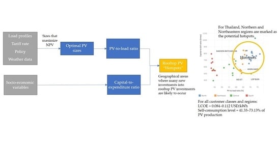


