Modelling Stochastic Electricity Demand of Electric Vehicles Based on Traffic Surveys—The Case of Austria

Abstract

Battery-powered electric mobility is currently the most promising technology for the decarbonisation of the transport sector, alongside hydrogen-powered vehicles, provided that the electricity used comes 100% from renewable energy sources. To estimate its electricity demand both nationwide and in individual smaller communities, a calculation based assessment on driving profiles that are as realistic as possible is required. The developed model based analysis presented in this paper for the creation of driving and thus electricity load profiles makes it possible to build different compositions of driving profiles. The focus of this paper lies in the analysis of motorised private transport, which makes it possible to assess future charging and load control potentials in a subsequent analysis. We outline the differences in demand and driving profiles for weekdays as well as for Saturdays, Sundays and holidays in general. Furthermore, the modelling considers the length distribution of the individual trips per trip purpose and different start times. The developed method allows to create individual driving and electric vehicle (EV) demand profiles as well as averaged driving profiles, which can then be scaled up and analysed for an entire country.

1. Introduction

The energy transition is widely seen as a shift in the energy sector from fossil-fuel towards renewable energy sources. Therefore, it is clear that all sectors and especially the transport sector also need to be decarbonised. Battery-driven electric mobility, along with hydrogen-powered vehicles, currently are the most promising technologies for the decarbonisation of the transport sector, as long as the electricity used is generated from 100% renewable energy sources. However, in the future, it will be necessary to rely, not only on a technological change, but also on alternative transport concepts, a different modal split, and public transport to achieve the emission targets, and avoid further congestion on the roads. Nevertheless, private transport will continue to represent a large share of the traffic volume in the future. The share of electric vehicles, which include battery electric vehicles (BEVs) and plug-in hybrid electric vehicles (PHEVs), is increasing steadily in the EU. While, in 2010 only 700 electric vehicles were newly registered, this figure increased to 550,000 vehicles in 2019. However, this still only represents a 3.5% market share of newly registered passenger cars of which about 2% were BEVs and 1% were PHEVs. The frontrunners in new registrations are Norway with 56% electric vehicles as measured by total newly registered vehicles, followed by the Netherlands with 18.53% and Iceland with 16.06%. Austria is in the middle of all EU countries with 3.43% of newly registered electric vehicles [1]. Regardless of current growth rates, a study by Eberhard and Steger-Vonmetz [2] outlines that, by 2050, the entire vehicle fleet in Austria will be electric.

To estimate the electricity demand that goes along with the substitution of fossil fuel-based private motorised transport with battery-driven electric mobility analysis on both, nationwide scale and in individual smaller municipalities, appropriate modelling requires reliable data regarding the driving behaviour.

This paper shows a method for estimating the actual demand profile of individual traffic at various detail levels. To provide optimal solutions for the interaction of EVs with the electricity grid it is important to design effective charging strategies.

These need some knowledge on driving behaviour. The core objective of this paper is to model driving patterns and electricity demand profiles of (future) electric mobility based on a survey on current mobility behaviour in Austria. Typical starting times, path lengths and trip purposes are considered. It also takes into account the differences in mobility behavior between weekdays and Saturdays and Sundays. Regional distribution of electricy demand caused by electric mobility, as well as effects of e-mobility on the electricity grid are not the focus of this paper. Also, the analysis of the electric vehicle charging behavior itself is not part of this paper.

Since e-mobility has played a significant role in discussing climate-friendly transport for quite some time [3,4], there is a broad selection of literature available dealing with different approaches to model BEV load and charge profiles.

Daina et al. [5] analyse different methodologies to model load and charge profiles of electric mobility. The models are categorized according to the time scale of the electric vehicle (EV) usage patterns and according to significant methodological differences that are applied. The modelling is broken down into travel statistics models, which are based on data from conventional vehicles. Further classifications range from activity-based approaches as daily or multi-day profiles derived from differences in lifestyle and activities to Markov Chain models. A Markov model is a stochastic model used to model changing systems randomly. It assumes that future states only depend on the current state, not on the events that occurred before. Considered states of a vehicle can include driving, parking in a residential area, parking in a commercial area and parking in an industrial area. The authors conclude that there is an urgent need to develop new modelling frameworks to take into account both, long-term strategic decisions of consumers and short-term decisions on EV use, as well as the design of price and non-price incentives for behavioural change. Activity-based modelling offers an attractive starting point to achieve this goal.

The paper by Pareschi et al. [6] deals with the question whether travel surveys provide a good basis for modelling EV driving patterns. The paper shows that existing Household Travel Surveys (HTS) and other travel diaries usually provide sufficiently accurate and abundant empirical information. However, they state that there is more uncertainty regarding the future role of EVs and critical parameters in the analysis like charging losses, charging rates and powertrain design. The paper concludes that conventional HTSs are a suitable basis to generate EV insights with some critical parameters to be considered.

A further Markov chain tool to estimate EV charging behaviour is presented by Sokorai et al. [7]. This tool enables the modelling of the stochastic nature of a charging station’s day-to-day usage if precise datasets of the driving behaviour are available. In addition, a case study to verify the algorithm is conducted. This study concludes that if adequate datasets on travel patterns with appropriate PEV statistics and real probability values are available as a model input, the algorithm can provide valuable stochastic information about electricity consumption at a given location.

Other papers based on the methodology of the Markov chain are presented by Schlote et al. [8] and Fischer et al. [9]. This paper presents a stochastic bottom-up model to evaluate the impact of EV’s on load profiles at different parking places and their potential for load management systems. This paper also considers socio-economic, technical and spatial criteria that influence the charging of electric vehicles. The model is used to analyse the effects of uncontrolled charging of EVs on the load profile of households. They find that uncontrolled charging causes a peak load increase up to a factor of 8.5 depending on the charging infrastructure.

The work carried out by Hu et al. [10] investigates the challenges that EVs add to the electricity grid at different penetration levels, taking into account the uncertainties caused by the stochastic charging and discharging behaviour. To cope with these uncertainties, a Monte Carlo-based simulation is used to generate EV charging and discharging profiles. The results in this paper show that the specific electricity grid studied can accommodate a high penetration of EVs by limiting charging to off-peak times. Lojowska et al. [11] also propose a Monte Carlo-based methodology in their paper for estimating the demand for electric vehicles based on a stochastic approach to modelling transport patterns. The focus of this paper is on the scenario of mainly domestic charging availability. The Monte Carlo simulation was performed for 1000 EVs and then scaled to a region with one million EVs. The authors conclude that total demand can increase if there are no incentives to spread the charging demand of EVs.

The work of Paevere et al. [12] presents a methodology to obtain spatial and temporal projections of the retail electricity demand of EVs, their load shift potential and the impact on household peak loads. The paper focuses on the territory of the State of Victoria, Australia and discusses differences in the potential for EV diffusion in different regions. In addition, regional statistics are used for the length of trips and arrival times and on this basis, EV charging and discharging is calculated. They conclude that the form and extent of EV demand profiles are subject to geographical variations. Areas where commuting is dominant generally have higher peak load demand, due to relatively longer trip distances and less diversity in home arrival times.

An agent-based approach using the established modelling tool NetLogo is applied in the paper of Chaudhari et al. [13]. The aim is to closely mimic the human aggregate behaviour and its influence on the electricity demand due to EV charging. The model implemented in this paper simulates and defines each EV by its charging characteristics, mobility behaviour and vehicle type. This creates an environment in which decision-making and various circumstances are taken into account to predict the charging behaviour of individuals as well as groups. The simulations in this paper were performed over a period of 24 h and for several days. The individual and total power demand of electric vehicles were determined for different scenarios. In addition, this model should allow for both commercial and private EVs with their different driving purposes. The authors conclude that the results highlight the practical applicability of the ABM-based approach to calculate the charging demand of EVs. Another agent-based approach to estimate EV’s charging demand is outlined by Lee et al. [14]. In this paper, an agent-based EV model is evaluated against real data observed during the “My Electric Avenue” project. The main finding is that, within the constraints of the available trial data, the agent model is able to replicate dominant charging pattern features.

Forecasting the electricity demand of EV’s is performed in the work by Moon et al. [15], Lopez and Fernandez [16], as well as in Cama-Pinto et al. [17] and Zhang et al. [18]. The latter was conducted for autonomous vehicles. Forecasting electricity demand using big data technologies is discussed by Arias and Bae [19]. Furthermore, charging EV’s in the smart city [20] and an empirically validated methodology to simulate electricity demand for electric vehicle charging are outlined in [21].

A user equilibrium model is discussed in [22]. In this paper, an approach is proposed that extends the User Equilibrium (UE) principle in order to determine, besides the flow over the network links, the service requests from the drivers to the various service stations.

In addition, there are several related publications that deal with similar topics. On-road charging of electric vehicles [23] using Contactless Power Train (CTP) where the total power demand for all the passing-by vehicles using the system is calculated and the possibility of powering the EVs directly from renewable energy sources is discussed. In [24], the optimal schedule of the charging behaviours of EVs with distinct energy consumption preferences in Smart Communities (SC) is outlined. In this paper, the authors propose a contract-based energy blockchain for secure EV charging in SC. An agent-based approach is proposed in [25] and discussed for EV deployment policies in Luxembourg. Day ahead bidding strategies for electric vehicle aggregators in uncertain electricity markets are outlined in [26], while in [27], the effects of electricity prices on the integration of high shares of photovoltaics are analysed.

The paper by Ramsebner et al. [28] directly builds on the methodology of this paper. The disaggregated demand profiles, as well as driving and parking times, were used as input for a linear optimisation model. This optimisation model aims to charge electric vehicles in a cost-optimal way, taking into account the SoC and considering different charging strategies.

As can be seen from the literature described, there are many different ways to model the demand and charging behaviour of electric mobility. Depending on the application and the systemic framework on micro or macro level, the models are able to answer a broad range of research questions. As already concluded in [5], modelling the driving behaviour of electric mobility on the basis of traffic surveys is agreed to be quite useful and sufficiently accurate. Therefore, the methodology presented in this paper is appropriate for our objectives and is also applied in the Urcharge project.

The main contribution of this paper lies in the transparent and straightforward modelling of load profiles, the easy calibration for different mobility behaviour, based on traffic surveys and in the high time resolution of the load profiles as a quarter of an hour.

The proposed methodology makes it possible to generate demand patterns for individual vehicles, different driving purposes but also for an aggregated average demand pattern including all driving purposes, which are scalable according to the share of EV’s in a region or in a whole country, in this paper, demonstrated by the example of Austria. Furthermore, different regional parameters can be applied to analyse demand patterns in different seasons or to distinguish between urban and rural areas. In addition, various distributions of routes and travel times within the driving purposes, as well as the mix of driving purposes on weekdays and weekends are taken into account. By focusing on individual vehicles and driving purposes, a holistic bottom-up analysis can be carried out on an aggregated level. The methodology presented in this paper strictly distinguishes between driving demand profile and charging profiles. The latter will not be discussed further in this paper. The strict separation between the generation of demand profiles and a subsequent generation of charging profiles allows the analysis of the effects of different charging management approaches. For example, uncontrolled charging, cost-minimized charging via a linear optimization model and corresponding pricing or the evaluation of load shifting potentials on different levels of aggregation.

The remainder of this paper is organized as follows. In Section 2, we introduce the methods of modelling the stochastic distribution of starting times as well as path lengths according to the trip purpose. Furthermore, we present the assumptions on the electricity consumption in winter and summer seasons as well as the composition of trips on different types of days. Section 3 shows model results and differences between driving purposes and between individual demand profiles and average demand profiles. Section 4 discusses and concludes the paper.

2. Materials and Methods

Basically, the model is developed to analyse individual demand profiles on the one hand and aggregated or average load profiles on the other hand to estimate the electricity demand by EVs.

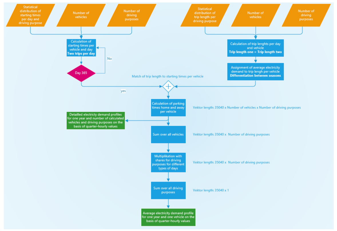
The fundamental procedure for creating an average load profile that can be scaled up to a municipal and countrywide level is described in Figure 1. First of all, the start times of the outward and return journey are calculated on a daily basis for different driving purposes, see

Table 1. Driving purpose and type of the day used for modelling e-mobility demand pattern.

Weekday	Saturday	Sunday
To the workplace/commuter
Drop-off and pick-up routes
Leisure
Business
Shopping
Visit
School/Education
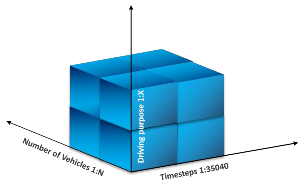
Errand

, whereby, a minimum time between these two times is specified, in order to guarantee a certain parking time. These start times are then assigned to different routes associated with route times and assumed grid-to-wheel consumption based on the calculated distance per route. The daily starting times and the resulting consumption are compiled into an annual driving profile. The calculation of the annual profiles is carried out in quarter-hourly resolution. This results in a vector of the size: 35,040 (24 h/day × 4 quarter hours/hour × 365 days) × number of calculated vehicles × number driving purposes (eight for the case of Austria) (see Figure 2).

This vector could then serve as input for a subsequent linear optimization model, which aims at charging the vehicles at minimal cost. The electricity demand at each time step is combined to an average total load profile based on the shares of the individual driving purposes, resulting in a vector of 35,040 time steps and x number of EVs. Finally, an average load profile is calculated across the number of vehicles, which can then easily be scaled with the EV penetration rate assumed. If the consumption of individual driving purposes is to be analysed, this can be done before averaging and by restricting the consumption vector.

2.1. Differentiation between Driving Purpose and Type of the Day

In order to generate load profiles for Austria, we use the latest traffic survey from 2014 [29]. This traffic survey examined and recorded the entire mobility behaviour for Austria divided into urban and non-urban regions. In addition, a distinction was made between working days, Saturdays and Sundays and seasonal differences. The study shows that in Austria about 104 billion kilometres are driven per year, with motorised private transport accounting for about 76 billion kilometres. Public transport represents approximately 21 billion kilometres, with 11 kilometres covered by railway. Pedestrian and bicycle traffic sum up to about 4 billion kilometres.

For the calculation of demand profiles for Austria, we assume that the essential parameters such as starting times, distance travelled and the parking times for e-mobility do not change significantly and use the following data and estimations for motorised individual transport to model the demand profiles.

According to the study [29], the following driving purposes are used for modelling, see Table 1:

As outlined in Table 1, eight driving purposes have been identified for Austria in general. The composition of the total trips from these eight driving purposes is different for weekdays, Saturdays, Sundays and public holidays, as shown in Section 2.4.

2.2. Stochastic Distribution of Starting Times

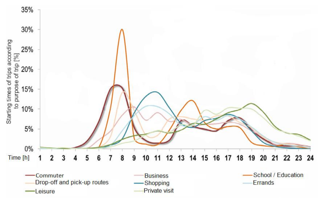
The different driving purposes also show different distributions of the start times, which have to be considered in the modelling. Figure 3 shows the start time distribution of the respective trip purposes for the outward and return journey, which are modelled as Gauss curves in a next step.

We use the Gauss distribution for a simple reproduction of the start time distribution for both the outward and return paths. For an even more precise reproduction of the curves, a superposition of several Gauss curves can be used.

The Gauss distribution is defined in Equation (1),

$$f(x|\mu ,{\sigma }^2)=\frac{1}{\sqrt{2\pi {\sigma }^2}}{e}^{-\frac{{\left(x-\mu \right)}^2}{2{\sigma }^2}},$$

(1)

using the variables:

• $\mu$ Average value
• ${\sigma }^2$ Variance
• $x$ Random value

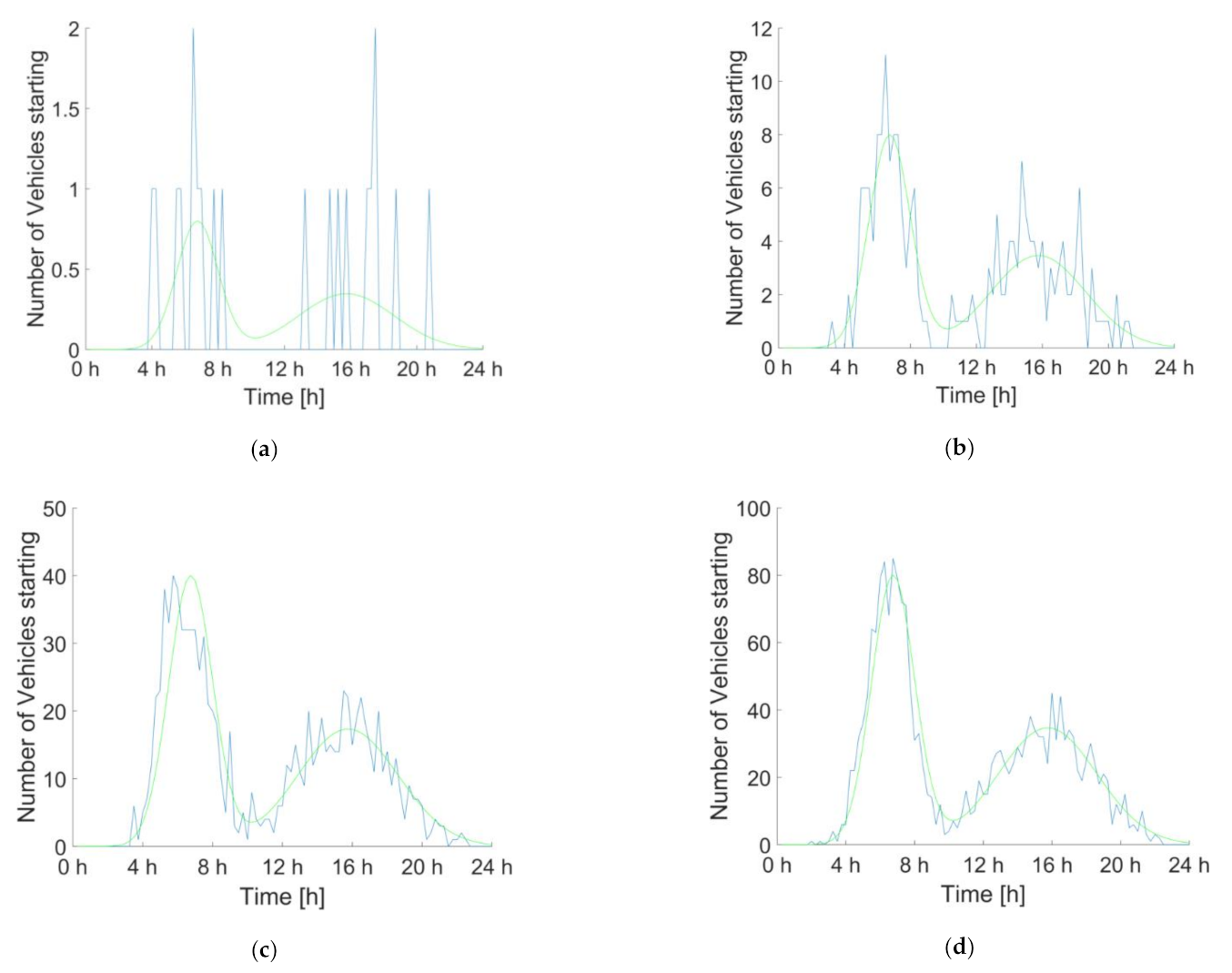
As illustrated in Figure 4 for commuters, the actual distribution of starting times depends strongly on the number of vehicles calculated. The more vehicles are calculated, the more the starting times actually match the applied distribution. For a realistic representation of the distribution in an overall load profile, a relatively large number of vehicles must therefore be calculated per trip purpose. With a time resolution of a quarter of an hour and a calculation of 1000 vehicles (representing 1000 battery storage systems with different State of Charge (SoC)) per driving purpose, this results in—35,040 (time steps per year) × 1000 (vehicles) × 8 (driving purposes)—over 280 million calculation points.

Just as for commuters, for all other driving purposes, mean value and variance or standard deviation are defined to determine Gauss distributions for the start times of the outward and return journey. The derived parameters are listed in

Table 2. Expected value and variance of the norm distributions of the start times of the individual routes per driving purpose.

Driving Purpose	Route One	Route Two
To the workplace/Commuter	$\mu =7:30 \mathrm{am}$ $\sigma =1 \mathrm{h}$	$\mu =4:00 \mathrm{pm}$ $\sigma =2.88 \mathrm{h}$
Drop-off and pick-up routes	$\mu =8:00 \mathrm{am}$ $\sigma =0.75 \mathrm{h}$	$\mu =3:30 \mathrm{pm}$ $\sigma =2.88 \mathrm{h}$
Leisure	$\mu =10:00 \mathrm{am}$ $\sigma =2.5 \mathrm{h}$	$\mu =7:00 \mathrm{pm}$ $\sigma =1.5 \mathrm{h}$
Business	$\mu =10:00 \mathrm{am}$ $\sigma =1.5 \mathrm{h}$	$\mu =3:00 \mathrm{pm}$ $\sigma =3.13 \mathrm{h}$
Shopping	$\mu =10:30 \mathrm{am}$ $\sigma =1.5 \mathrm{h}$	$\mu =5:00 \mathrm{pm}$ $\sigma =2.5 \mathrm{h}$
Visit	$\mu =11:00 \mathrm{am}$ $\sigma =2 \mathrm{h}$	$\mu =5:30 \mathrm{pm}$ $\sigma =4.25 \mathrm{h}$
School/Education	$\mu =8:00 \mathrm{am}$ $\sigma =1.5 \mathrm{h}$	$\mu =3:30 \mathrm{pm}$ $\sigma =4.25 \mathrm{h}$
Errands	$\mu =10:30 \mathrm{am}$ $\sigma =1.5 \mathrm{h}$	$\mu =4:00 \mathrm{pm}$ $\sigma =2.5 \mathrm{h}$

. The mean start time is given as a time of the day, in the model this time as well as the variance is converted into quarter-hourly values. For example, 6 a.m. is converted to the 24th quarter-hour value of the day (6 h × 4) and a standard deviation of 2.4 h is rounded to 10 quarter-hours.

2.3. Distribution of Driving Distances

In order to take into account the fact that not all trips are of the same length, we also introduce a statistical distribution of the distances travelled depending on the purpose of the trip, based on the original data.

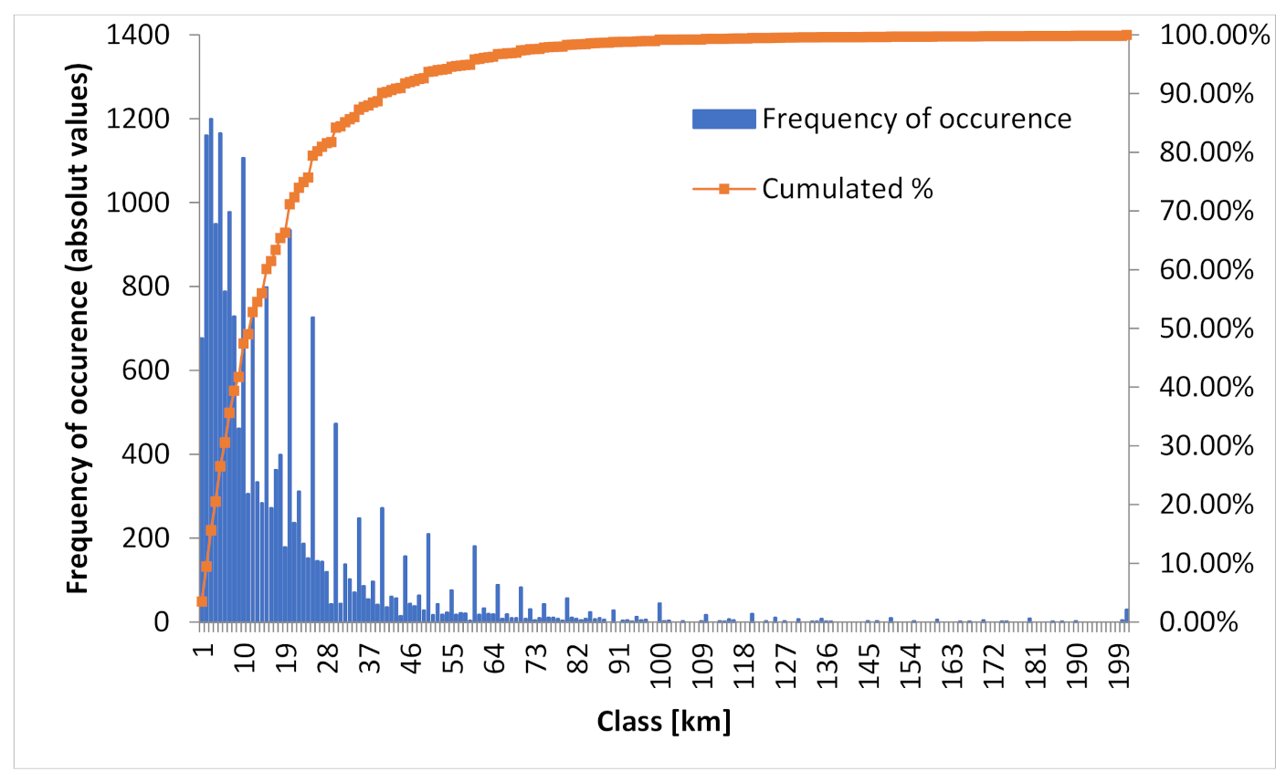
The analysis of the empirical data results in different distributions of the distances travelled depending on the purpose of the trip and the day of the week. For the sake of simplicity, all trips per purpose of the trip were summarised and analysed according to their distribution, regardless of the type of the day. To reproduce the distribution as precisely as possible, the distances were divided into 200 classes of 1 km each, see Figure 5 as an example for the distribution of trip lengths for commuter traffic.

The actual length of each route per driving purpose was then based on the class average. For the class between zero and one kilometre for example the actual length is 0.5 km. The maximum driving length was limited to 200 km because the analysis of the data showed that only few trips (e.g., 0.16% in the case of commuters) exceeded 200 km.

Since the discrete distribution of the trip lengths was determined, the multinomial distribution was chosen as a function to model the statistical allocation of the trip lengths to the individual daily trips.

The multinomial distribution is a generalisation of the binomial distribution. If mutually exclusive results are possible for a random process m and the random process is repeated n times independently, the probabilities can be calculated using the multinomial distribution. Each possible event x1, …, xk has a probability of occurrence of p1, …, pk. The probability of the occurrence of a certain distance is known. The n-repeats are recalculated for each day according to the number of cars. In this way, each trip gets assigned to a random length according to the distribution.

The multinomial probability distribution is defined as follows; see Equation (2),

$$\mathrm{f}\left(n_1,\dots ,n_k|N;p_1,\dots ,p_k\right)= \frac{n!}{n_1!\dots n_k!}{\displaystyle \prod }_{i=1}^k{p}_i^{n_i} , {\displaystyle \sum }_{i=1}^k{n}_i=n , {\displaystyle \sum }_{i=1}^k{p}_i=1$$

(2)

• $n$ Number of vehicles
• $k$ Number of path length
• $p$ Probability of occurrence of path length

According to the study, the average annual distance travelled by car is 13,300 km/a. With an average distance of 16 km for individual motorised traffic per trip, this means that an average of 2.28 trips are made per day.

Since we assume only 2 trips per day in the modelling, the return path is assigned the same distance as the outward path. This results in an average length of 16 km across all driving purposes. In order to be able to represent the average driving performance of 13,300 km per year, the average annual route length and thus all route lengths need to be scaled up by a factor of 1.14.

2.4. Share of Driving Purposes on Overall Trips

Although the driving purposes and start times remain the same for working days, Saturdays, Sundays and holidays, the respective shares vary considerably. For example, the share of commuter traffic on the overall trips on a working day is much higher than on a Saturday or even a Sunday or public holiday. This shift in the shares of driving purposes results in different demand profiles for weekdays, Saturdays, Sundays and holidays.

In order to calculate the respective shares of the driving purposes, one must first consider the total routes for all transport modes and then break them down to motorised individual traffic, which, however, is not outlined directly in the statistics.

Based on the number of trips per trip purpose from

Table 3. Number of total routes and share of driving purposes in total route.

Trip Purpose	Working Day	Working Day	Saturday	Saturday	Sunday	Sunday
	Share of total trips [%]	Number of trips	Share of total trips [%]	Number of trips	Share of total trips	Number of trips
Total trips/day	100	22,090,000	100	19,851,000	100	14,885,000
of which
To the workplace/Commuter	26	5,743,400	7	1,389,570	5	744,250
Drop-off and pick-up routes	7	1,546,300	5	992,550	5	744,250
Leisure	15	3,313,500	29	5,756,790	47	6,995,950
Business	5	1,104,500	2	397,020	2	297,700
Shopping	16	3,534,400	29	5,756,790	3	446,550
Visit	8	1,767,200	15	2,977,650	26	3,870,100
School/Education	8	1,767,200	0.5	99,255	0.5	74,425
Errands	13	2,871,700	12	2,382,120	11	1,637,350

, the average trip length of 16 km for motorised private transport is used to calculate the kilometres travelled per day. However, since the trips are only partially covered by private motorised transport, the total distance covered per day must be aligned with the respective shares, see

Table 4. Kilometres per day and respective share of motorized individual traffic on total trips.

Trip Purpose	Working Day	Working Day	Saturday	Saturday	Sunday	Sunday
	Share of motorised individual transport in total trips [%]	Distance [km]	Share of motorised individual transport in total trips [%]	Distance [km]	Share of motorised individual transport in total trips [%]	Distance [km]
Kilometres/day individual transport		162,299,648		137,003,662		95,537,884
of which
To the workplace/Commuter	60	55,136,640	60	13,339,872	60	7,144,800
Drop-off and pick-up routes	67	16,576,336	67	10,640,136	67	7,978,360
Leisure	30	15,904,800	30	27,632,592	30	33,580,560
Business	70	12,370,400	70	4,446,624	70	3,334,240
Shopping	45	25,447,680	45	41,448,888	45	3,215,160
Visit	45	12,723,840	45	21,439,080	45	27,864,720
School/Education	9	2,544,768	9	142,927	9	107,172
Errands	47	21,595,184	47	17,913,542	47	12,312,872

, in order to be able to derive the kilometres driven per day, see Equation (3). As the traffic-survey does not show whether the distribution differs between Saturdays, Sundays and holidays, the same distribution as on working days is used for the calculation of kilometres travelled.

$$D=N \times s \times l$$

(3)

• $D$ Distance travelled by vehicle and day [km]
• $N$ Total number of trips completed per day [1]
• $s$ Share of motorised individual traffic in total number of trips travelled [1]
• $l$ Average distance travelled per trip by motorised individual traffic [km]

From the distribution of kilometres per driving purpose for individual traffic, the shares of the respective driving purpose are deducted, see

Table 5. Share of driving purposes in the total routes of motorised individual traffic in %.

Trip Purpose	Working Day	Saturday	Sunday
Share of individual transport per day	100.0	100.0	100.0
of which
To the workplace/Commuter	34.0	9.7	7.5
Drop-off and pick-up routes	10.2	7.8	8.4
Leisure	9.8	20.2	35.1
Business	7.6	3.2	3.5
Shopping	15.7	30.3	3.4
Visit	7.8	15.6	29.2
School/Education	1.6	0.1	0.1
Errands	13.3	13.1	12.9

. In the end, these shares serve to generate an average demand profile for one vehicle.

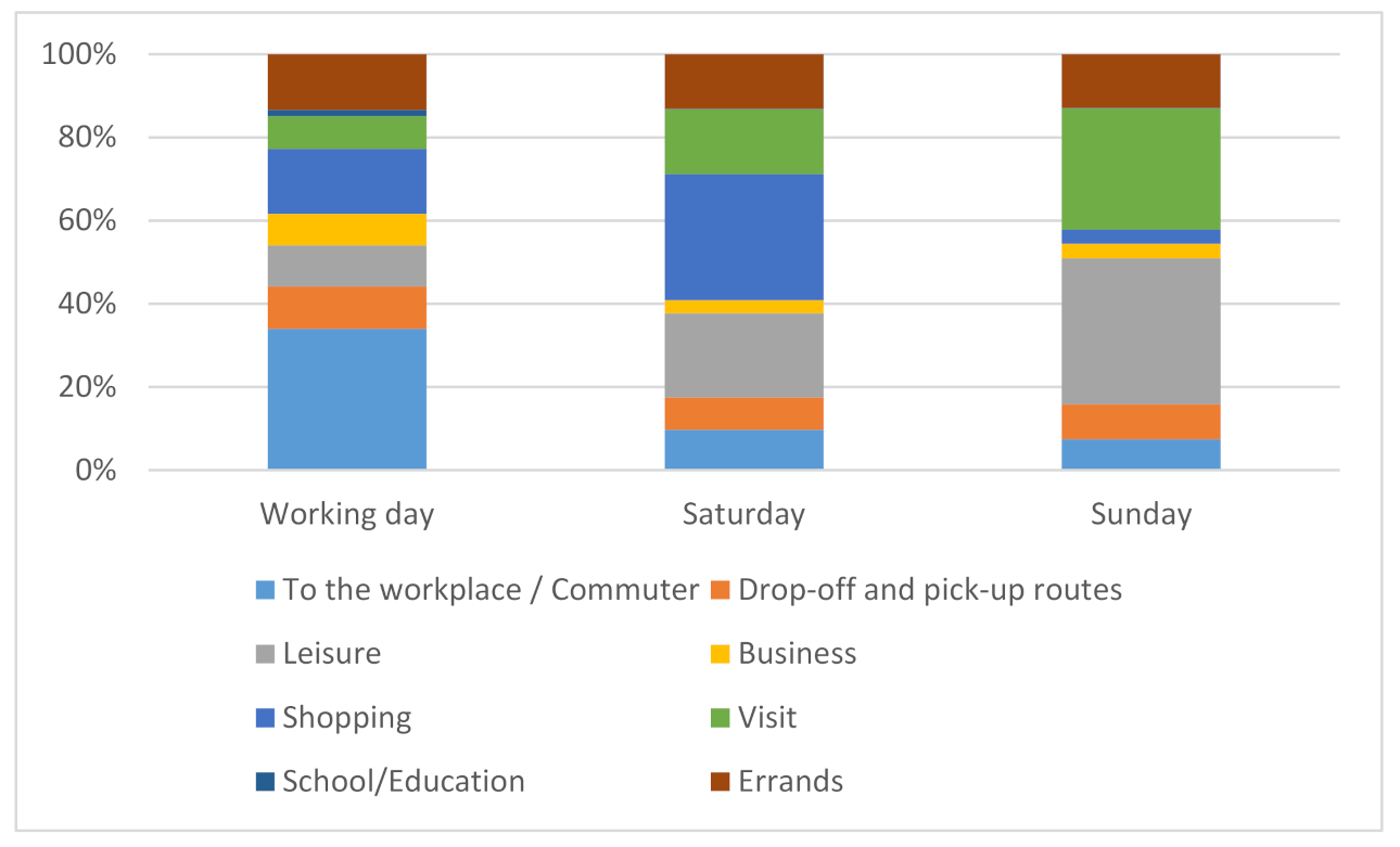
As can be seen from Table 5, commuter traffic dominates on working days, followed by shopping and private errands. On Saturdays, shopping dominates with over a third of the trips made, followed by leisure trips and private visits. On Sundays, on the other hand, leisure trips are at the top of the list almost the same as visiting trips. See also the graphical visualization in Figure 6.

2.5. Electric Vehicle Consumption

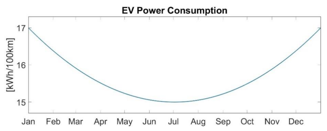
The grid-to-wheel consumption of the vehicles in this paper is assumed to be the same for all driving purposes and vehicles. Even if there certainly are differences in the consumption of individual vehicles, as well as different routes, it seems justifiable for the present modelling to assume these as average consumption, as this would also be averaged in the large number of vehicles calculated. However, it is not the aim of this study to analyse the consumption of different vehicle models. Nevertheless, we consider the fact that consumption tends to be higher in winter than in summer as also outlined in the study of the American Automobile Association (2019) [30] and Iora and Tribioli (2019) [31]. These studies do not focus specifically on Austria, but on the differences in the electricity demand of electric vehicles in summer and winter. Since, to the best knowledge of the authors, there is no representative study for Austria, an average pattern was assumed, which is believed to represent the climatic conditions and circumstances in the western federal provinces with their alpine character, as well as in the eastern regions with a rather mild climate and the different types of vehicles.

For this reason, consumption throughout the year is interpolated between a maximum of 17 kWh/100 km in winter and a minimum of 15 kWh/100 km in summer, see Figure 7.

3. Results

As already discussed in the previous chapters, this methodology provides an excellent starting point to answer many different research questions, especially regarding optimal load management. On the one hand, it is possible to analyse single trip purposes, single vehicles, and groups of vehicles regarding their quarter of an hour, daily or yearly electricity demand, driving distances, starting times, or even standing times at home or away from home. On the other hand, it is possible to analyse average load profiles for specific trip purposes, mixed trip purposes, and an average overall load profile that can easily be scaled up for a whole region or country, in this case Austria. In the following chapter, the modelling results are presented by means of individual and average load profiles. For this purpose, 1000 individual vehicle demand profiles were created for each trip purpose.

3.1. Individual Demand Profiles versus Average Demand Profiles

From the methodology chapters, it is quite clear that the individual driving profiles change in length per trip and the starting times, depending on the driving purpose. How this affects load profile modelling is analysed in more detail in the following sections.

Annual aggregated and averaged model results based on the input data already discussed show that the distances travelled and the annual consumption per trip purpose vary enormously (see

Table 6. Model results for eight driving purposes considering the underlying 1000 randomly generated profiles.

Trip Purpose	Min. Distance of Vehicles [km/a]	Max. Distance of Vehicles [km/a]	Average Distance of Vehicles [km/a]	Average Distance per Trip [km]	Min. Demand of Vehicles [kWh/a]	Max. Demand of Vehicles [kWh/a]	Average Demand of Vehicles [kWh/a]	Average demand per trip [kWh]
to the workplace/commuter	10,430	16,080	12,973	17.8	1627	2509	2032	2.79
drop-off and pick-up routes	5476	9426	7246	10	854	1477	1135	1.56
Leisure	8422	14,750	11,338	15.6	1320	2315	1776	2.44
Business	13,600	23,674	18,228	25	2135	3711	2855	3.92
Shopping	4442	7234	5581	7.7	690	1134	874	1.2
Visit	9526	17,332	12,806	17.6	1497	2744	2006	2.76
School/Education	13,508	21,420	16,993	23.3	2113	3362	2662	3.66
Errands	6006	11,006	8152	11.2	942	1714	1277	1.75

). The shortest distance of a single-vehicle is observed for drop-off and pick-up routes with 5476 km/a, whereas the longest distance is observed for business routes (23,674 km/a). The modelled average distance per trip of 16 km is precisely in line with the study results [29]. The large number of vehicles calculated (1000) results in a relatively good statistical distribution of both the start times and the trip lengths. The annual consumption of individual vehicles varies between 690 kWh/a and 3711 kWh/a, and the variation of annual consumption depends not only on the route length but also on the different grid-to-wheel consumption in summer and winter. The average consumption per trip is 3 kWh across all driving purposes.

Depending on the analysis and the kilometres driven, these results must be adjusted or scaled to the respective regional conditions. In our case, as we will see later, we will adapt these results specifically to Austria, also considering the type of the day as an input parameter. Since we have simulated only 2 instead of 2.28 routes per day for simplicity, there is a deviation in the average annual kilometres driven (11,665 km calculated vs. 13,300 km [29]), and thus, also in the annual average consumption. If individual vehicles are to be analysed, it is possible, on the one hand, to select the vehicle (from the 1000 calculated) that comes closest in terms of distance, or on the other hand, to scale it with the number of kilometres required. If driving purposes are to be analysed more precisely, the average demand profile must be scaled with the actual distance driven or the actual consumption.

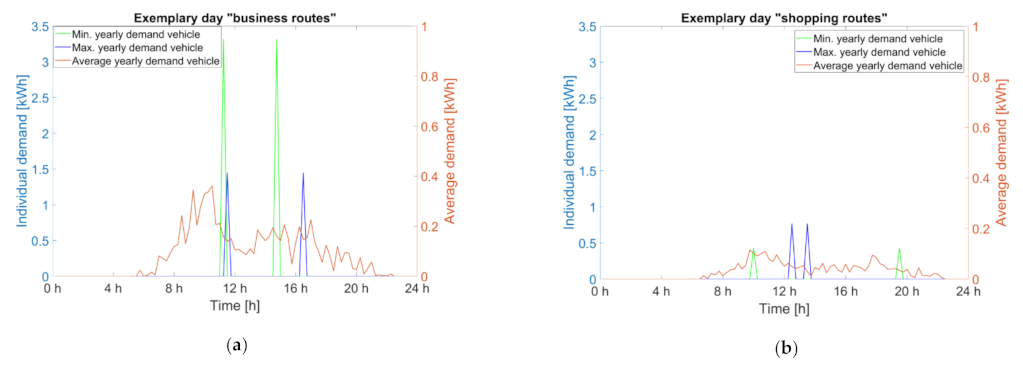
In the following, the results at vehicle level are compared to the mean value of the total calculated vehicles per trip purpose. For reasons of clarity, only the “shopping routes” and “business routes” are compared. In Figure 8 and Figure 9, the green and blue lines represent a vehicle’s consumption per day and year respectively. The orange line represents the average value per 1000 vehicles per trip purpose. The y-axes on the left side represent the demand of the individual vehicles while the y-axes on the right side of the graph represent the average vehicle’s demand. The two individual vehicles were selected out of 1000 in such a way that the vehicle with the overall lowest annual consumption (green line) and the vehicle with the overall highest annual consumption (blue line) are evaluated in order to get a feeling for the differences in the respective peaks and in the frequency of the peaks that occur.

The electricity demand during the trip is only assigned to one quarter of an hour in the model. However, the previously calculated distance and the average speed of 60 km/h result in corresponding trip times of one minute per km. Together with the electricity demand, the length of the journeys and the times when the vehicle is on the road, the parking times at home and away from home are calculated and assigned to the individual vehicles.

Figure 8 and Figure 9 show how individual demand profiles and averaged demand profiles behave within a day and over a year. The daily perspective shows that due to the distribution of the start times and the distribution of the path lengths, the averaged load profile for a trip purpose has a significantly different characteristic than the individual vehicle. It becomes clear that the peak load of a vehicle can be significantly higher than the peak load of an average load profile. The average load profile tends to follow a continuous load curve, whereas an individual vehicle’s profile is limited to a few points in time during the day. The peaks of individual vehicles at individual points in time are no longer as significant in an average load profile. In addition, it can be seen that a vehicle with a low annual consumption also has higher peak loads on some days than a vehicle with a generally higher annual load profile due to the distribution of the path lengths, as compared with Figure 8a. Figure 8 also shows that the heights of the peaks, as well as their occurrences, can vary greatly. In the comparison between business trips and shopping trips, it becomes clear that peaks are significantly higher in the business profile and also occur significantly more frequently. This is also reflected in the average profile, which is significantly higher. It is important to note that the current analysis does not take into account differences in weekdays and weekends. These differences will be identified in the next section.

The advantage of disaggregated modelling of demand profiles lies precisely in the fact that it is possible to extract any information about a vehicle at any time, e.g., current consumption, driving, parked at home and parked away. No information about demand peaks is lost. For subsequent precise analysis of the charging behaviour, a disaggregated demand profile is necessary to be able to calculate the individual charging power at vehicle level depending on the SoC of the battery and afterwards aggregate the total charging power of a vehicle pool. This is difficult to do with an aggregated calculation because the detail of the information is already missing and an average load profile only offers an aggregated representation. However, it is not always necessary to provide all information at a disaggregated level. It is not possible to include several 1000 individual EV demand profiles per country in large energy system models. In such cases, it definitely makes sense to use an aggregated profile.

3.2. Yearly Average Demand Profile for Austria Considering Different Types of Days

In Section 3.1, the different load profiles were presented based on the trip purpose and on individual and average load profiles.

For the analysis of the electricity demand of many vehicles in urban sections, cities or rural areas and on country level, it makes sense to create an average annual load profile, which consists of all trip purposes. Since the shares of driving purposes differ for weekdays, Saturdays and Sundays (see Section 2.4), the total demand profile also differs on these types of days.

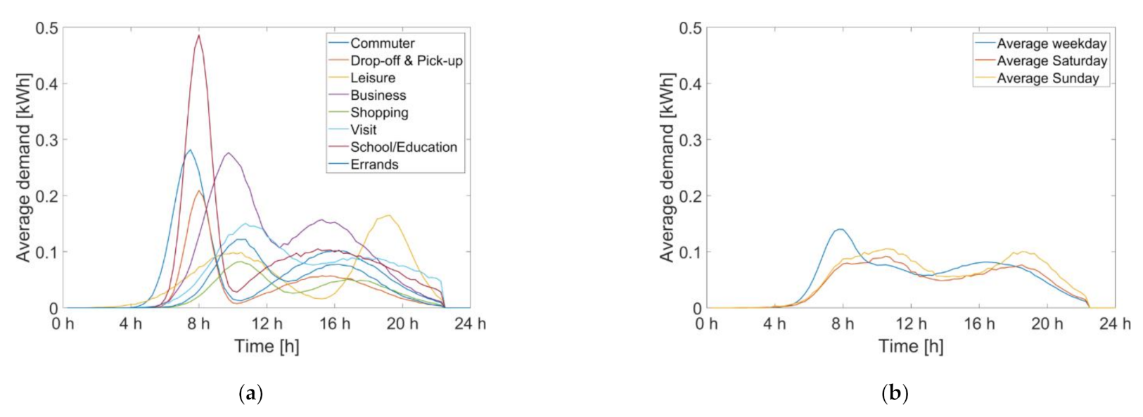
Figure 10 shows the consumption of an average day for the different trip purposes on the left side individually and not specifically for weekday, Saturday and Sunday. In the morning, school and commuter trip drop-off and pick-up routes dominate, which of course, correlates with the selected start distribution and the path length distribution modelled according to Figure 3. We now combine the individual distributions of the individual trip purposes’ load profiles, taking into account the shares from Table 5 and obtain different averaged load profiles for weekdays, Saturdays, and Sundays, see Figure 9b. Due to commuter dominance with about 34% in the morning, there is an apparent increase on weekdays compared to Saturdays or Sundays. As mentioned previously, the parking times at and away from home are calculated at vehicle level based on the start times and route lengths. This information is required to know when and for how long the vehicle is available for subsequent analyses regarding the charging management of individual vehicle groups.

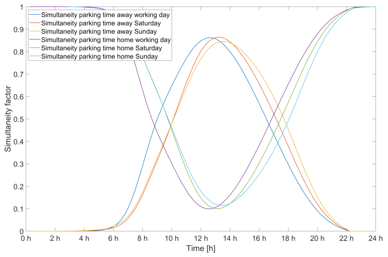
For the visualisation in Figure 11, however, an aggregated form of the parking times was chosen to clarify how the entirety of the vehicles behaves concerning typical parking times.

As can be seen in Figure 11, there are slight differences in the availability of vehicles while parked at or away from home. On weekdays, there is a peak around lunchtime in the simultaneity of vehicles parked away from home. The gradient is also slightly higher than on Saturdays, Sundays and public holidays due to commuting. Especially in the evening and at night, almost all vehicles are parked at home. As can be seen in Figure 10, by summing up the curves at and away from home, the vehicles are parked mostly either at home or away from home, e.g., at the workplace. Only very few times a day, the vehicles are actually in motion.

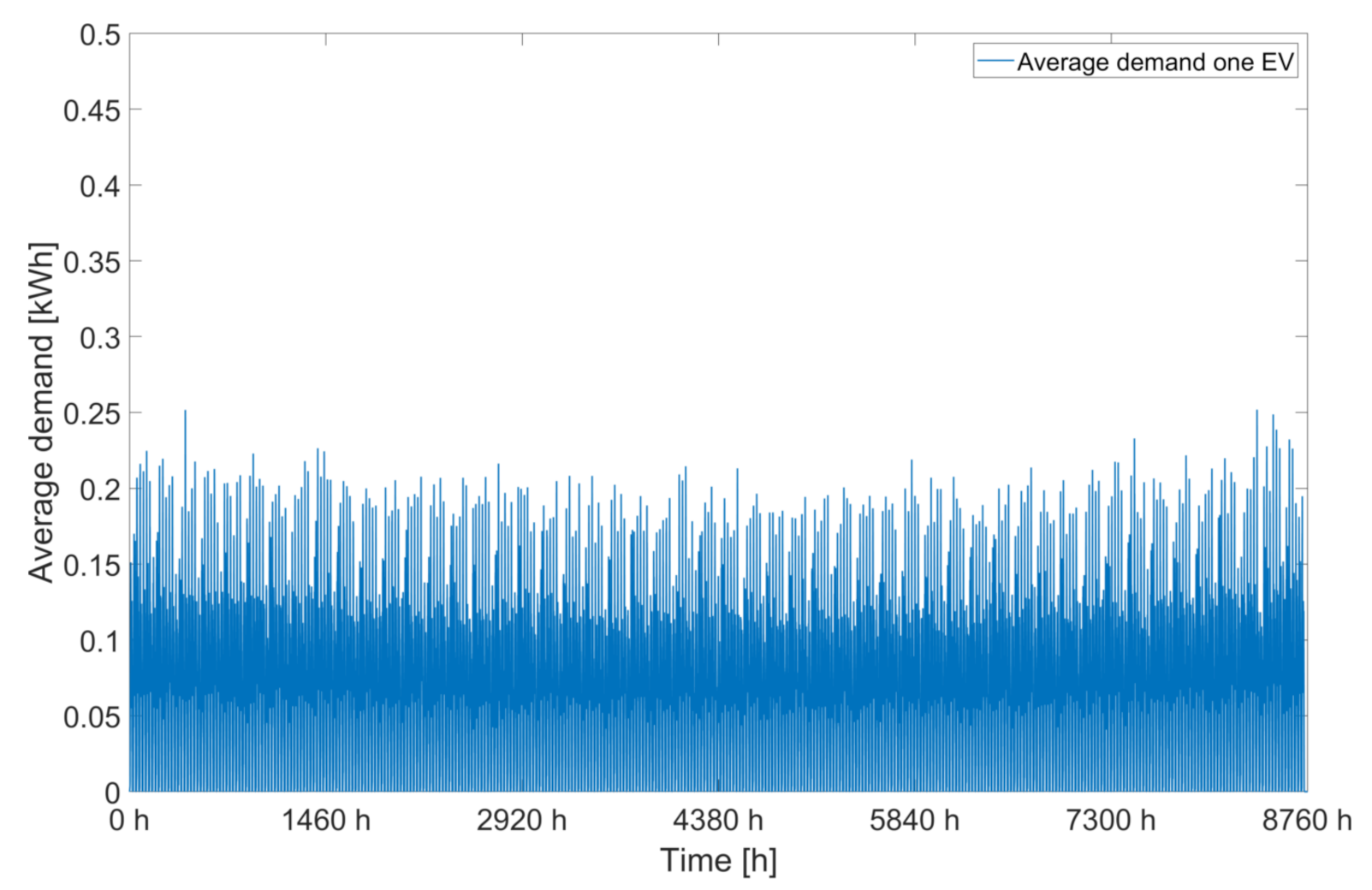
The individual days’ composition into a continuous annual load profile leads to an annual mileage of approx. 10,570 km/a, which is significantly lower than the mileage of an average vehicle in Austria. Furthermore, it is also less than the average distance of the combined consideration of the different path purposes in Table 6. This can be explained by the fact that the length distribution and the different shares of the path purposes in the total profile compose different shares. Therefore, the length also deviates from the previously calculated length where only an average of all path purposes was calculated. To create an Austria-wide aggregated load profile and scale the load profile for different EV penetration rates, this average load profile must first be calibrated to a travelled distance of 13,300 km. Therefore the load profile is calibrated with the factor 1.26 (13,300 km/10,570 km), resulting in the load profile in Figure 12.

Based on this load profile, different scales can now be applied to answer different (research) questions for different regions. From the authors’ point of view, the aggregated model results serve mainly as input for system modelling where no detailed individual or disaggregated analysis of demand or driving behaviour is required.

As already outlined, for detailed modelling of individual vehicles or vehicle networks’ charging behaviour, the disaggregated output of the model should serve as input for further analyses. Such an analysis was implemented, for example, by Ramsebner et al. [28] where the disaggregated demand profiles, as well as driving and parking times, were used as input for a linear optimisation model. This optimisation model aims to charge electric vehicles in a cost-optimal way, taking into account the SoC and considering different charging strategies. To calculate this cost-optimal charging, a disaggregated, high-resolution demand profile is needed as input, which was created by the methodology presented in this paper.

4. Discussion and Conclusions

The methodology, presented in this paper, aimed at modelling and calibrating high-resolution EV demand profiles based on traffic surveys and at making these profiles versatile in application. These demand profiles should then be available as input parameters for energy system models.

The results presented show, that EV demand profiles can be created and evaluated in high temporal resolution per vehicle and trip purpose or on aggregated level as an average load profile. The advantage of the high resolution, disaggregated use of the load profiles is primarily that the information about individual load peaks is maintained and that start, travel and arrival, and parking times can be mapped with quarter-hour accuracy. In addition, the bottom-up approach has the advantage that a wide variety of aggregated load profiles can be created, which is de facto not possible in the other direction.

In addition, the calibration and creation of these load profiles can be conducted with other country or regional data. As we have seen, the decisive parameters are, on the one hand, the starting times, the distribution of the trip lengths, and, on the other hand, the shares of the different trip purposes among the trips per day. The more precise these data are available, the better the reality can be reproduced in the load profiles.

In order to reproduce this methodology for other countries or regions, the following data is required:

• A breakdown on the driving purpose as precise as possible
• Data on the starting times of the individual routes as accurate as possible
• Data on the distribution of trip lengths as accurate as possible
• Shares of trip purposes on different days

Alternatively, this data could be generated beforehand, or assumptions on average trip lengths must be made. If the data on starting times cannot be modelled using Gaussian distributions, for example, a different, e.g., discrete, distribution can be used to model the trip lengths.

The division of the path lengths into path classes and their distribution must also be adapted to the respective data situation. Often, only rugged ranges of the trip length distribution are given in evaluations. In this case, the path class width, as well as the path class centre must be adjusted accordingly and the trip length calculated accepting higher inaccuracy.

In any case, it is important to analyse the data in advance in order to choose the right type of distribution and to assess possible limitations of accuracy due to assumptions and data inaccuracies. The computing time and computing capacity must be taken into account. This means that it is not always possible and reasonable to calculate 1000 vehicles per trip purpose to resolve 35,040 time steps. The high time resolution as well as the amount of vehicles results in more than 280 million data points that have to be calculated. This may be necessary and feasible for the calculation of an average load profile. On a disaggregated level, for example in a subsequent linear optimisation model, the calculation of so many data points, however, reaches the limit of the computational capacity. When simultaneously calculating the cost-optimal charging of 8000 storage units with different SoC’s and a resolution of 35,040 time steps, taking into account additional constraints, the calculation time can be exorbitantly high or no solution to the problem can be found. In particular, two things have to be considered before selecting the appropriate method. What purpose do the created demand profiles serve and what data is available. Furthermore, the quality of the input data plays an important role. Depending on the type and accuracy of the available data, the methodology presented here can directly be used. The probability that not all data are available on this level of detail for every analysis is high, and thus, in the case of any data gaps, corresponding assumptions or simplifications must be made, for example concerning the start times or the path length distribution.

Finally, it can be concluded that in order to develop effective charging strategies to reduce the pressure on the electricity grid and to effectively use renewable generation, electrical load profiles for EVs are needed. The methodology presented in this paper provides an excellent opportunity to establish such demand profiles on different levels of detail. Based on this paper, we find a need for future research in the consideration of plug-in hybrid vehicles, different charging strategies, as well as Vehicle to Building (V2B) and Vehicle to Grid (V2G) applications, to achieve an optimal integration of electro mobility into the energy system and use the available flexibility options efficiently.

External effects that would also change user behaviour were not taken into account in this paper. However, it is evident that the Covid pandemic and the associated lockdowns, for example, have changed mobility behaviour. This is perhaps less true for the distribution of starting times than for the average distances and lengths of trips. Due to lockdown restrictions, many people switched to home office, and commuters drive to work less frequently. Private visits and shopping trips are also limited. If one also assumes that the modal split will change in the future and public transport will be increasingly expanded and incentivised, the average distances travelled by car will tend to shorten. This will lead to a general reduction in peak loads for EV electricity demand, fewer kilometres driven, and a subsequent reduction in annual electricity demand.