1. Introduction
Inductive power transfer (IPT) systems have been widely used to transfer power without physical contact. The IPT system overcomes many disadvantages of traditional physically contacted power transfer systems that cause sliding wear, contact sparks, and several other dangers caused by dirt and moisture. Several researchers have investigated different aspects of IPT systems. For example, Chen et al. proposed using a third coil to improve misalignment tolerance of IPT systems [
1]. Shevchenko et al. investigated compensation topologies in IPT systems [
2], and Hao studied an IPT power supply for wireless electric vehicles [
3].
Recently, several researchers have focused on advanced controller designs for IPT systems. For example, Li et al. investigated a robust controller for IPT systems to improve the problems of parametric uncertainty, load disturbance, and misalignment [
4]. Based on a closed-loop IPT system with a two-degree-of-freedom control structure, good performance can be obtained, even though the mutual inductances vary and load changes. Xia et al. implemented a
-synthesis control method of an LCL IPT system. The
-synthesis control method was based on structured singular values [
5]. Their experimental results showed that the proposed IPT system could quickly and accurately track the reference voltage. Li et al. studied a two-degree-of-freedom
controller for an IPT system with parameter perturbations [
6]. Based on a state-space model, a two-degree-of-freedom
controller, which was very complex, was developed. Nail et al. proposed an optimal static state-feedback controller design for a multivariable IPT system [
7]; however, that paper did not demonstrate experimental results.
Predictive controllers present several advantages that make them suitable for motor drives and power electronic applications, including IPT systems. The concepts of predictive controllers are intuitive and easy to understand. They can be applied for different IPT systems that include input constraints and nonlinearities. Although the design of predictive controllers requires prediction, a performance index, and optimization, its realization is very simple when a digital signal processor is used [
8,
9]. To the authors’ best knowledge, there are no or only a few researchers who have investigated predictive controller designs for IPT systems. To fill this research gap, a predictive controller design for an IPT system is proposed here. By using the augmented variables, the state equation of an IPT system is easily developed. Next, the predictive controller is designed based on a performance index. Finally, a model-based predictive controller is designed. By using a digital signal processor (DSP), the predictive controllers are implemented, which provide better performance than proportional-integral (PI) controllers, including faster responses and better load disturbance responses. To the authors’ best knowledge, the ideas demonstrated in this paper are original and have not been discussed in previously published papers [
1,
2,
3,
4,
5,
6,
7,
8,
9].
2. The Three-Winding IPT
Only a few researchers have focused on the comparison of a two-winding IPT and a three-winding IPT. Chen et al. proposed a three-winding IPT system to improve its misalignment tolerance and efficiency [
1]. In reference [
1], the authors demonstrate that the third-coil improves the misalignment performance and also affects the characteristics of the compensation circuit. In this paper, a three-winding IPT, shown in
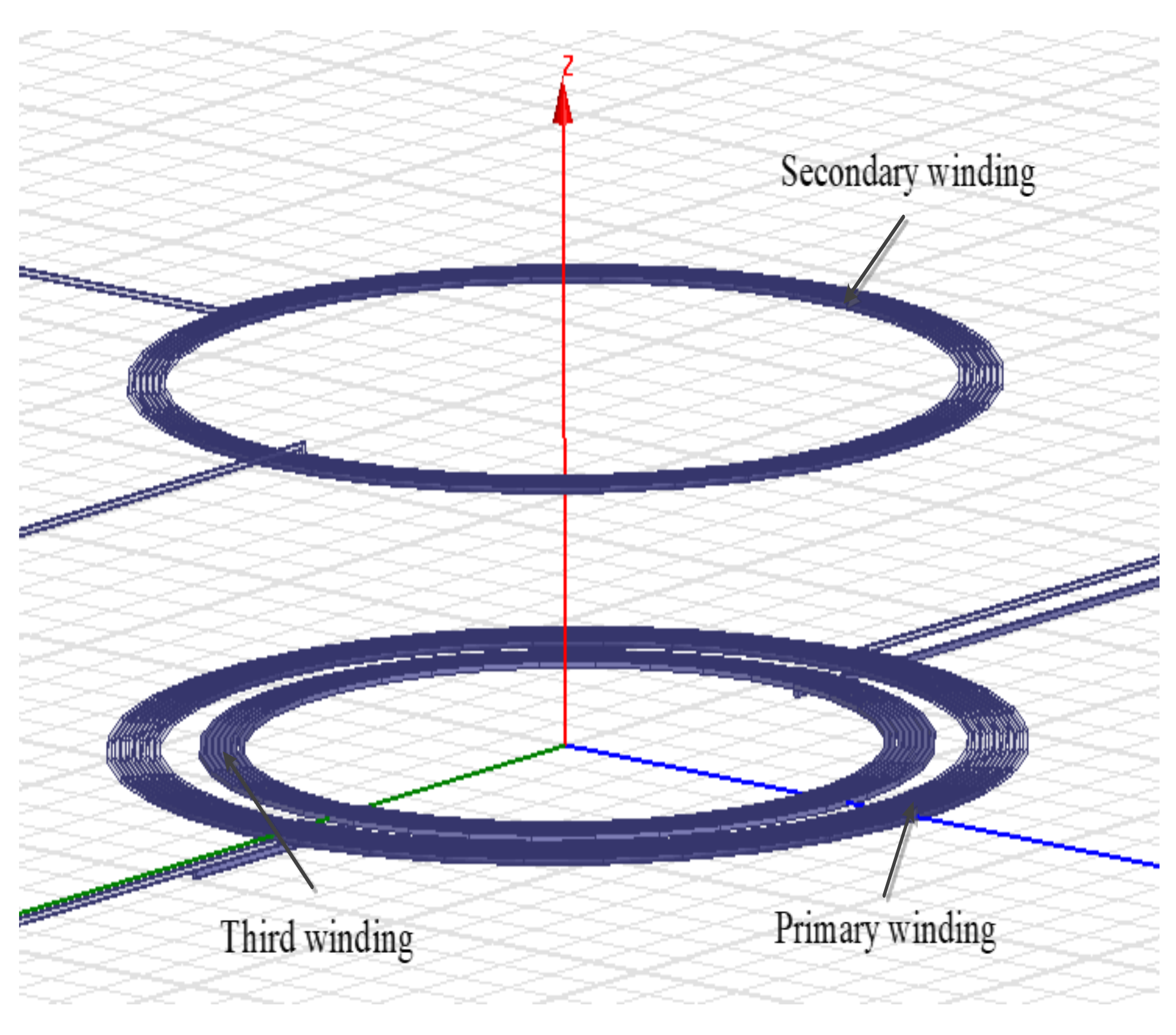
Figure 1, is used. This IPT does not use any core. A comparison of a two-winding IPT and a three-winding IPT is not shown in this paper because they have different characteristics. As a result, this paper only focuses on the three-winding IPT. The three-winding IPT provides several advantages. In
Figure 1, the third winding of the IPT system provides a high current
, which is over 12 A from the experimental results in this paper. The major reason is that the third winding is short-circuited when the winding is in resonance. The current
provides an extra current to the primary winding. However, when the third winding is operated at a frequency that is different from the resonant frequency, the internal impedance is increased, and then the current in the third winding is reduced. In fact, the third winding enhances the flux-linkages in the primary winding compared to an IPT, which does not use a third winding. Moreover, the third winding also provides reactive power, supplies phase angle compensation, and increases the kVA capability in the primary winding, all of which effectively reduces the deterioration of the output power when the IPT has a larger air gap or a misalignment between the primary winding and the secondary winding [
10]. It is well known that the third winding of a transformer can be used to compensate for the influence of disturbances of an output load, such as harmonics and a three-phase unbalanced load for a power system. The major reason is that the third winding can stabilize voltages, supply the third harmonic currents to magnetize the transformer core, filter third harmonics from the system, and provide grounding action. The detailed explanations are shown in reference book [
10]. In this paper, we use the same concept and use a third winding to provide the reactive power to reduce the deterioration of air gap variations and misalignment between the primary winding and secondary winding of an IPT system.
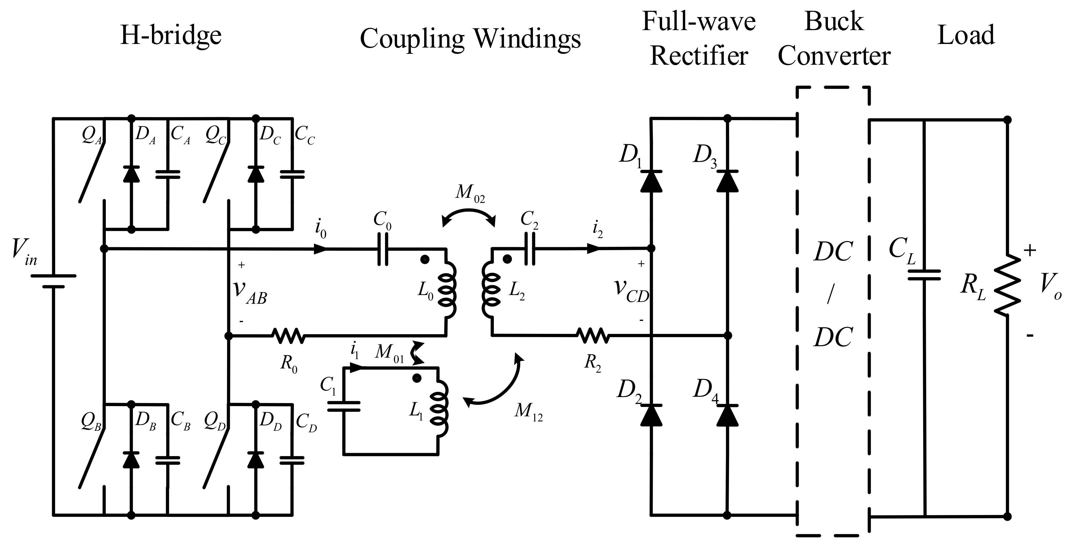
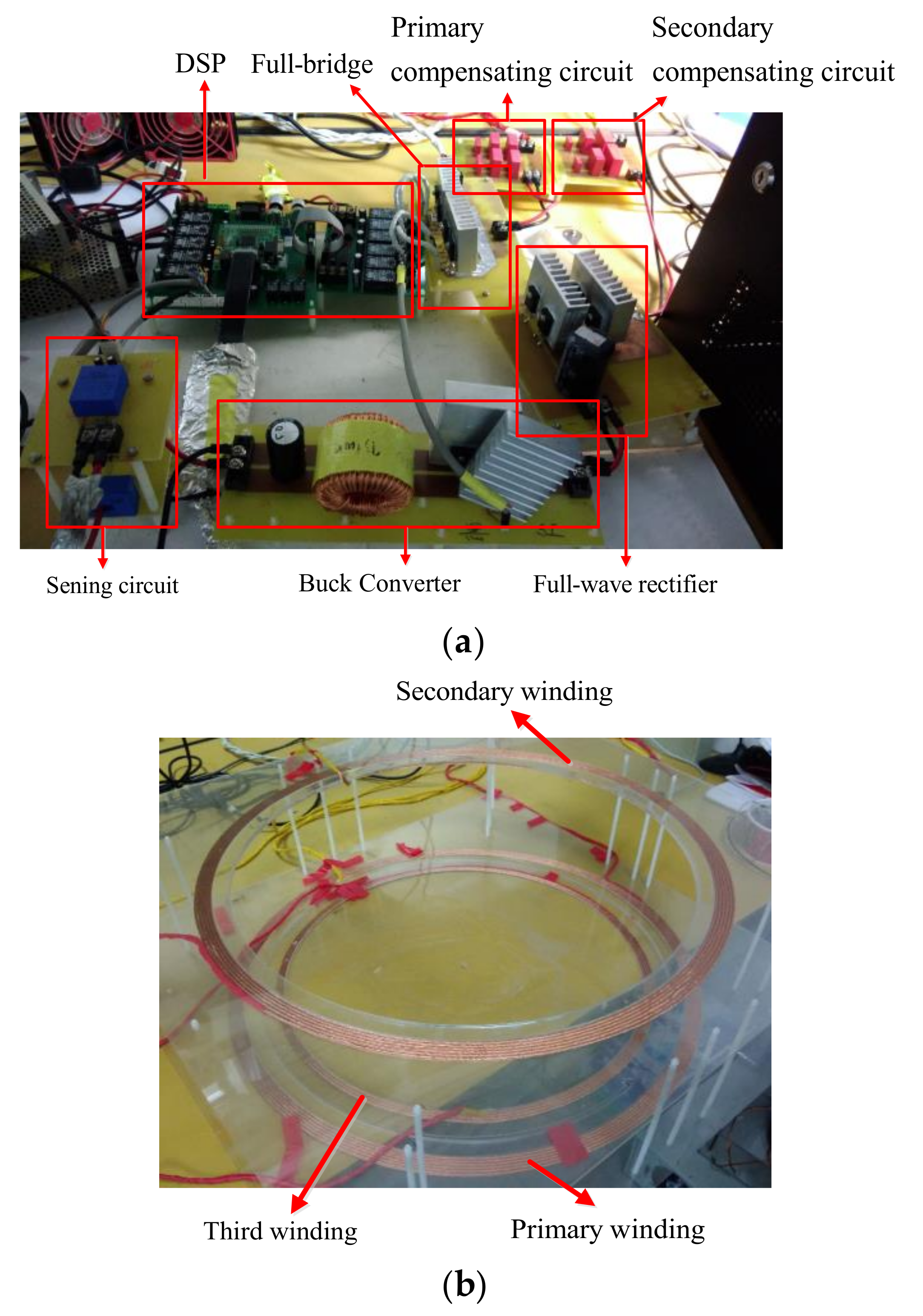
The main circuit of the three-winding IPT is shown in
Figure 2, which includes an H-bridge, three windings, a full-wave rectifier, a DC/DC buck converter, a filtering capacitor, and a resistor. By suitably designing the H-bridge circuit, zero-voltage switching can be obtained since the diode is turned on before the MOSFET turns on. In addition, the primary winding is arranged near the third winding to increase their mutual inductance. The DC/DC buck converter is used to reduce the output voltage so that it matches the load voltage.
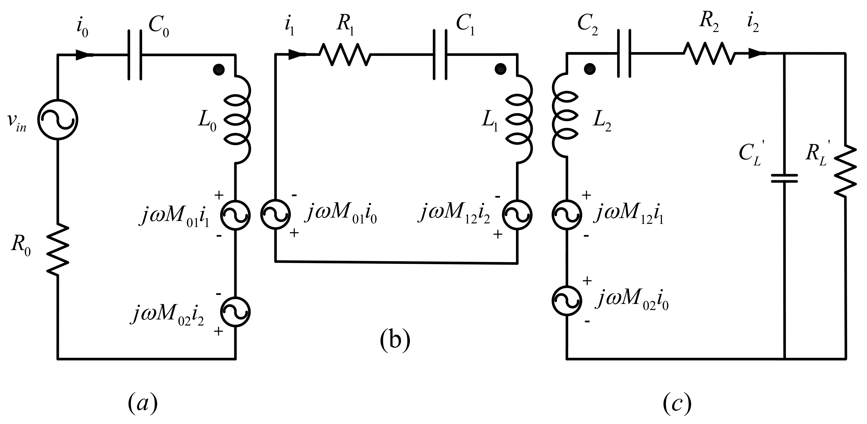
Figure 3a–c show the whole AC equivalent circuit of the three windings.
Figure 3a shows the equivalent circuit of the primary winding.
Figure 3b shows the equivalent circuit of the third winding.
Figure 3c shows the equivalent circuit of the second winding. In
Figure 3a–c,
is the equivalent resistance of the primary winding,
is the equivalent resistance of the secondary winding,
is the equivalent resistance of the third winding,
is the equivalent capacitance of the primary winding,
is the equivalent capacitance of the secondary winding,
is the equivalent capacitance of the third winding,
is the AC equivalent capacitance of the filtering capacitance
, and
is the AC equivalent resistance of the load
.
At a resonant frequency, the reactance of leakage inductance is equal to the reactance of the compensating capacitor. As a result, the equations of the three-winding circuit are expressed as follows:
and
From (2) and (3), one can obtain the
and
as follows:
and
In Equation (4), the product of multiplying
and
is very small because both parameters are less than
. Moreover, in Equation (5), the product of multiplying
and
is also very small. As a result, Equations (4) and (5) can be simplified as follows:
and
Inputting (6) and (7) into (1), one can obtain
From (8) and by assuming the input reactive power is zero, one can obtain the input power as follows:
The output power of the three-winding is
Inputting (7) into (10), one can derive the output power as
From (9) and (11), the efficiency of the three-winding can be obtained as follows:
From (12), we can observe that the efficiency of the IPT is related to the parameters of , , , , , ,, and . However, when the parameter is increased, the efficiency always increases.
3. Design of Predictive Controller of a Three-Winding IPT System
Predictive control has been in development for over four decades. It belongs to the class of model-based control, which requires precise parameters of the uncontrolled plant. This control has been applied in the manufacturing of paper, food, and furnaces, and in petrochemical and mining industries for forty years [
11,
12]. This type of control has many advantages. For example, it can be used for single-input and single-output processes and multi-input and multi-output processes. It is the only method that can handle constraints in a systematic way during the design of a controller. Recently, this predictive control has been widely used in power converters and electrical drives because of the powerful computational abilities of digital signal processors (DSPs) [
13]. In this paper, a predictive voltage controller and a predictive current controller are used as a part of the considered inductive power transfer system. The details are as follows:
From
Figure 2, the time-lag of the H-bridge is very short because the H-bridge is switched to a 77 kHz high-frequency. As a result, a major delay-time comes from the inductance of the DC/DC buck converter, the filtering capacitance
, and the output resistance
. The transfer function of the whole IPT system, therefore, is expressed as follows:
where
is the output voltage,
d is the duty cycle of the buck converter,
is the input DC voltage,
s is the differential operator,
L is the inductor of the buck converter,
is the output capacitor of the buck converter, and
is the output resistor load. The relationship between the duty cycle and the analog signal, which is used to compare the triangular carrier, is
where
is the peak value of the PWM carrier, and
u(s) is the analog signal that is used to compare the triangular carrier. From (13) and (14), one can obtain
Taking the z-transform of Equation (15) and considering the zero-order hold, one can obtain
and
where
T is the sampling time of the voltage-loop of the IPT, which is 14
. From (16), one can obtain the output voltage of the IPT
, which is related to the parameters
,
,
, and the control input
u(k) as follows:
By choosing the vector
and using a state-space representation, one can rewrite the state equation of (21) as follows
and
The output equation of (21) can be expressed as
and
From (22), one can derive
From (26), by using a similar method, one can obtain
Then, we can define the augmented variable as follows:
Then from (30), we can obtain
and
The output is expressed as follows:
and
From (31), we can derive the predictive state variable vector as follows:
The predictive output can be expressed as
Submitting (36) into (37), we can derive
and
We can define the performance index
as follows:
where
is the reference command. By choosing
=
and submitting (38)–(40) into (41), one can obtain
where
is the weighting factor and
X(k) is the state variable vector, which includes two state variables,
and
. In the real world, the control input
is the summation of
and can be expressed as follows:
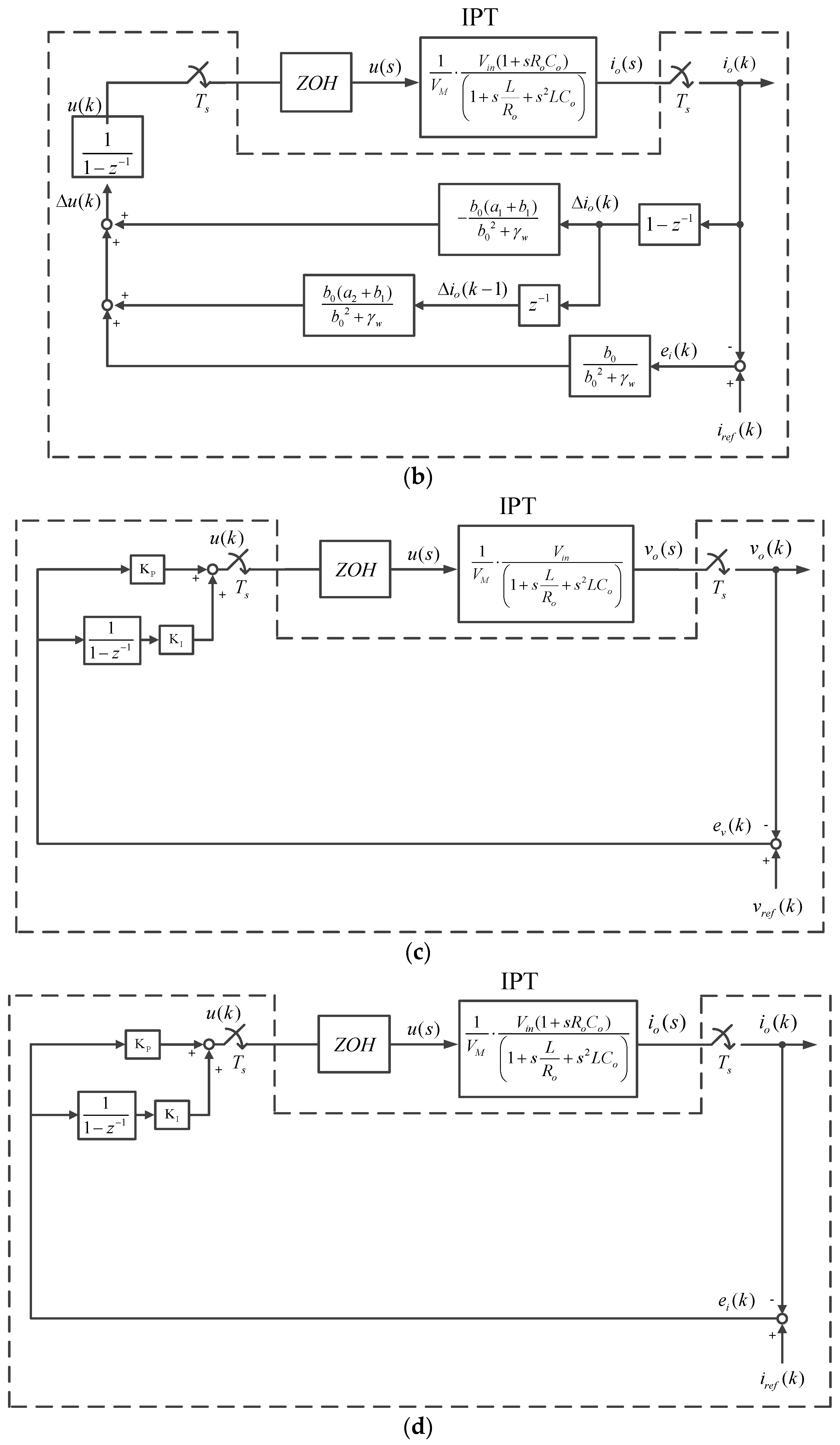
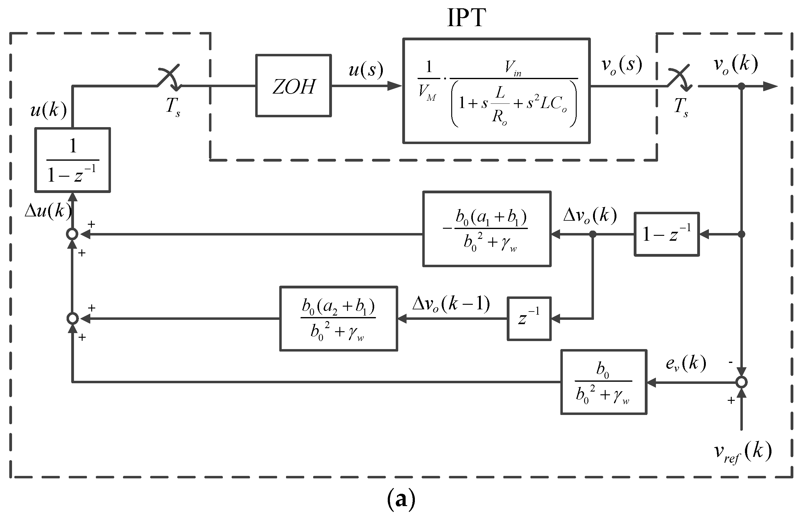
The proposed voltage predictive controller, which is shown in Equation (42), is shown in
Figure 4a. By using Equation (42), the proposed current predictive controller can be obtained and is shown in
Figure 4b, which is very similar to the predictive voltage controller design in our study and can be used as a constant current controller of a battery set.
Figure 4c,d show the block diagrams of the implemented PI controllers, which are used for comparison. It may be unfair to compare a predictive control system with a simple PI controller tuned using the pole placement method. In the future, more advanced control methods, such as optimal control, adaptive control, or robust control could be used and compared with the predictive control proposed in this paper.
5. Simulations and Experimental Results
In this paper, Matlab software, which is a powerful computing tool, was used to carry out the simulation. The block diagram of the simulation is shown in
Figure 6. First, the reference voltage command is compared to the output voltage of the IPT system to obtain the error
. Next, the error
is multiplied by
to obtain
(k). The
which is the difference between the output voltage
and
, is multiplied by
to obtain
(k). The delay of
which is
is multiplied by
to obtain
(k). After that, the
, which is the summation of the
(k), , and
(k) can be computed. Finally, the control input
, which is the integration of the
, is sent to the plant, which is the IPT, to produce the output voltage
. A closed-loop IPT system is thus obtained.
Several experimental results are shown here to validate the theoretical analysis and simulated results. The switching frequency of the H-bridge is 77 kHz, the sampling interval of the current-loop is 14
, and the sampling interval of the voltage loop is also 14
. The simulated waveforms use the resistance, self-inductance, and mutual inductance of the coils by using the off-line measurement of the real IPT system. The predictive step is one step ahead, and the control horizon is one. The uncontrolled plant has the following transfer functions. For voltage control, the transfer function is
and for current control, the transfer function is
The predictive controller uses two weighting factors— = 0.1 and = 0.3—for the voltage control system to compare their voltage responses. The smaller weighting factor produces a quicker voltage response, which means that the control input energy is less important and the output voltage response is more important. The predictive controller uses the weighting factors: = 0.01 and = 0.03 for the current control system to compare their current responses. The smaller weighting factor produces a quicker current response, which means that the control input energy is less important and the output current response is more important. The PI controller of the voltage-loop includes
and The PI controller of the current-loop includes and
The parameters of and are obtained by using a pole assignment method.
Several simulated and measured results are demonstrated in this paper.
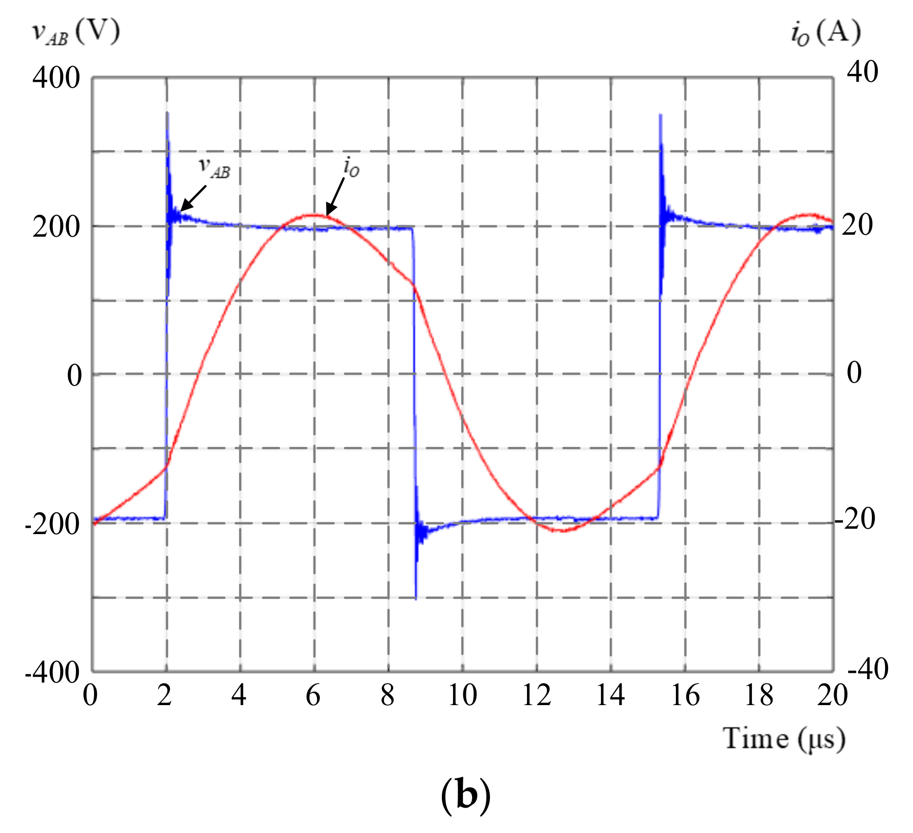
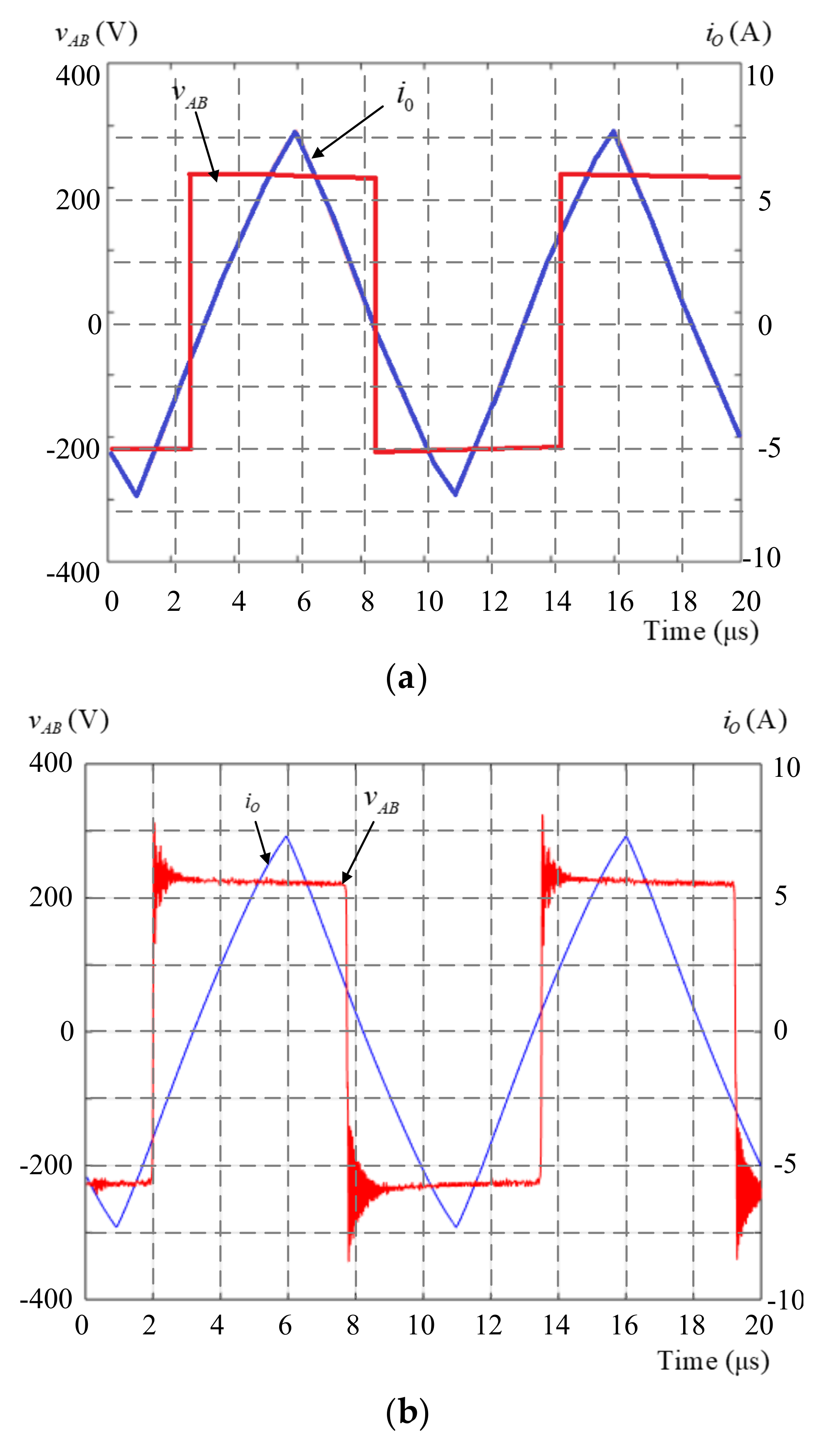
Figure 7a,b show the H-bridge output voltage
and output current
at 200 W.
Figure 7a demonstrates the simulated waveforms, and
Figure 7b demonstrates the measured waveforms. The
is a symmetrical square-wave voltage, but the
is a symmetrical triangular current due to the light load. The simulated and measured waveforms are quite similar; however, the measured output voltage
has obvious ringings due to the resonance of the stray capacitance and stray inductance. The ringings can be reduced if the layout of the main circuit is improved.
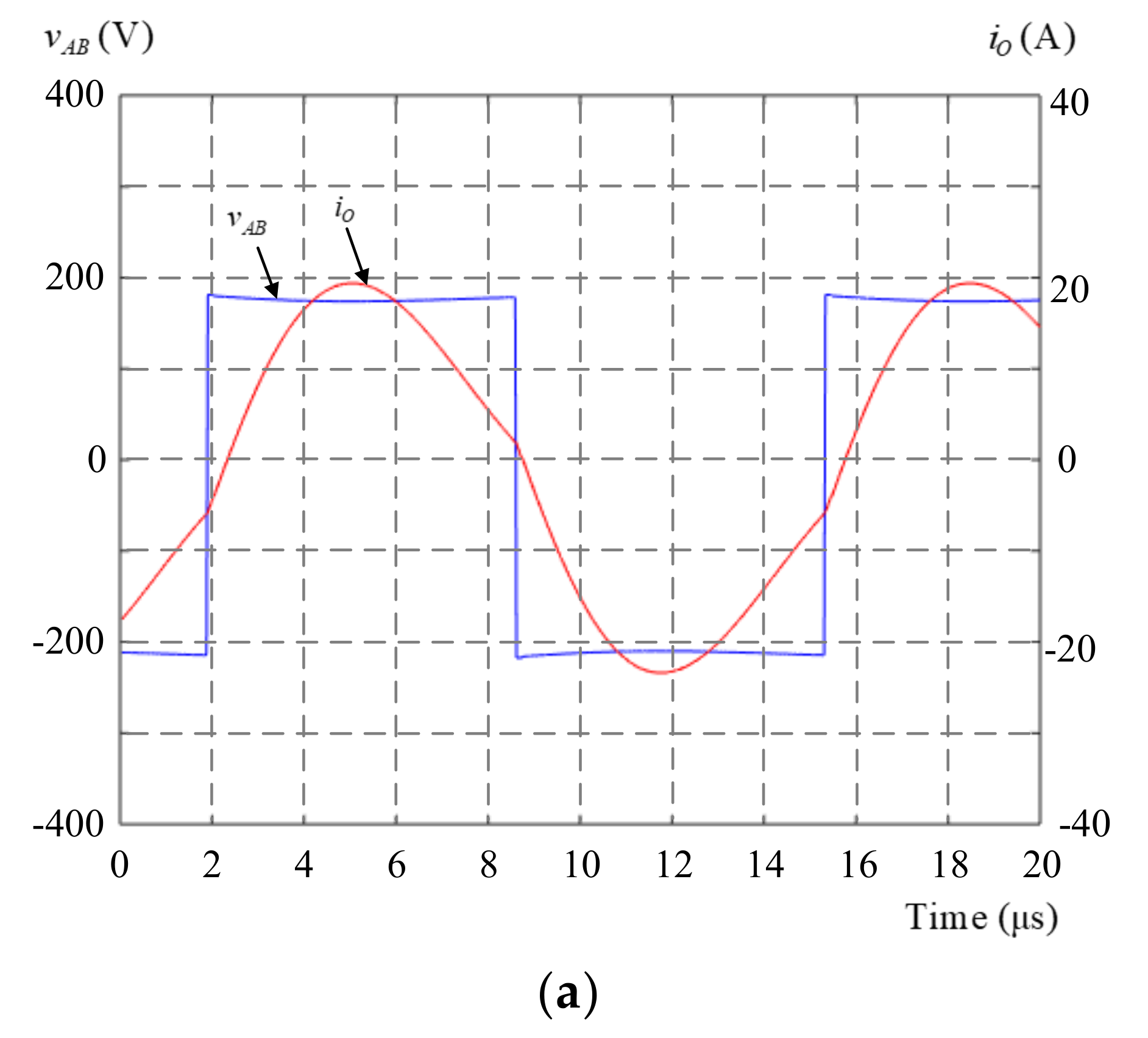
Figure 8a,b show the H-bridge output voltage
and output current
at 2 kW. The
is a symmetrical square-wave voltage, but the
is a near sinusoidal current due to the heavy load.
Figure 8a demonstrates the simulated waveforms, and
Figure 8b demonstrates the measured waveforms. They are also similar; however, the measured output voltage
has obvious ringings again.
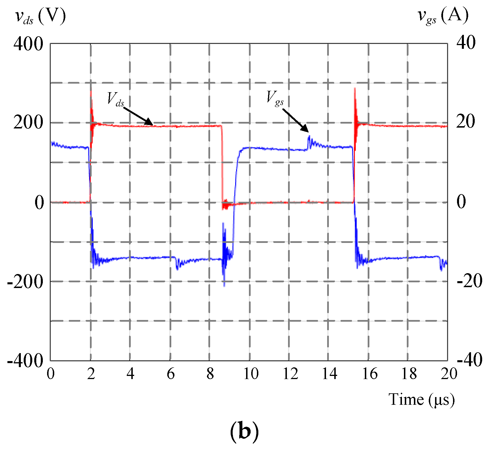
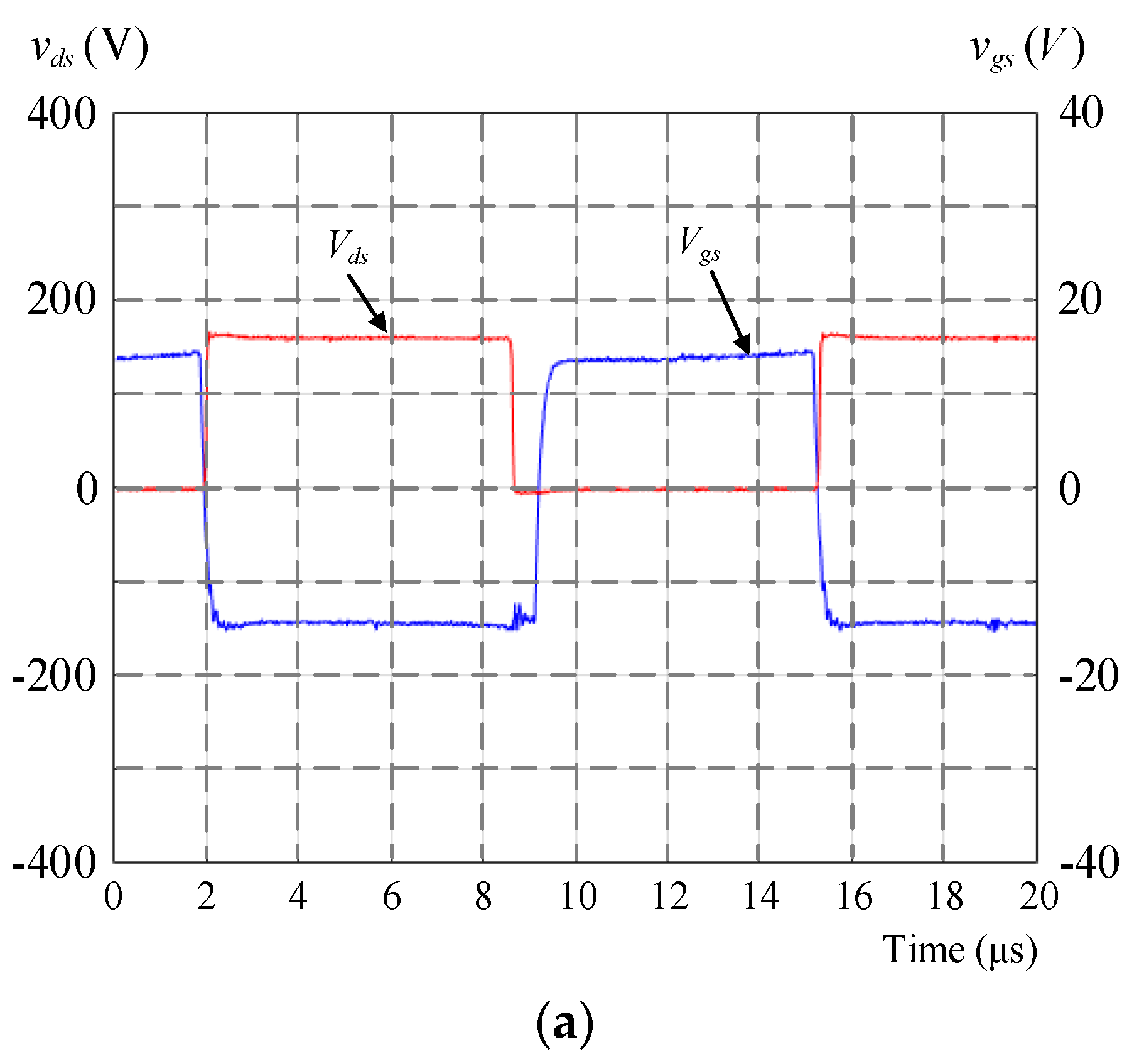
Figure 9a,b show the measured waveforms under zero voltage switching conditions at 200 W and 2 kW. Both figures show that the
reaches a zero voltage when the
gating signal is turned on, which implies that a zero voltage switching can be obtained. The measured voltage
has obvious ringings when the power switch is turned on.
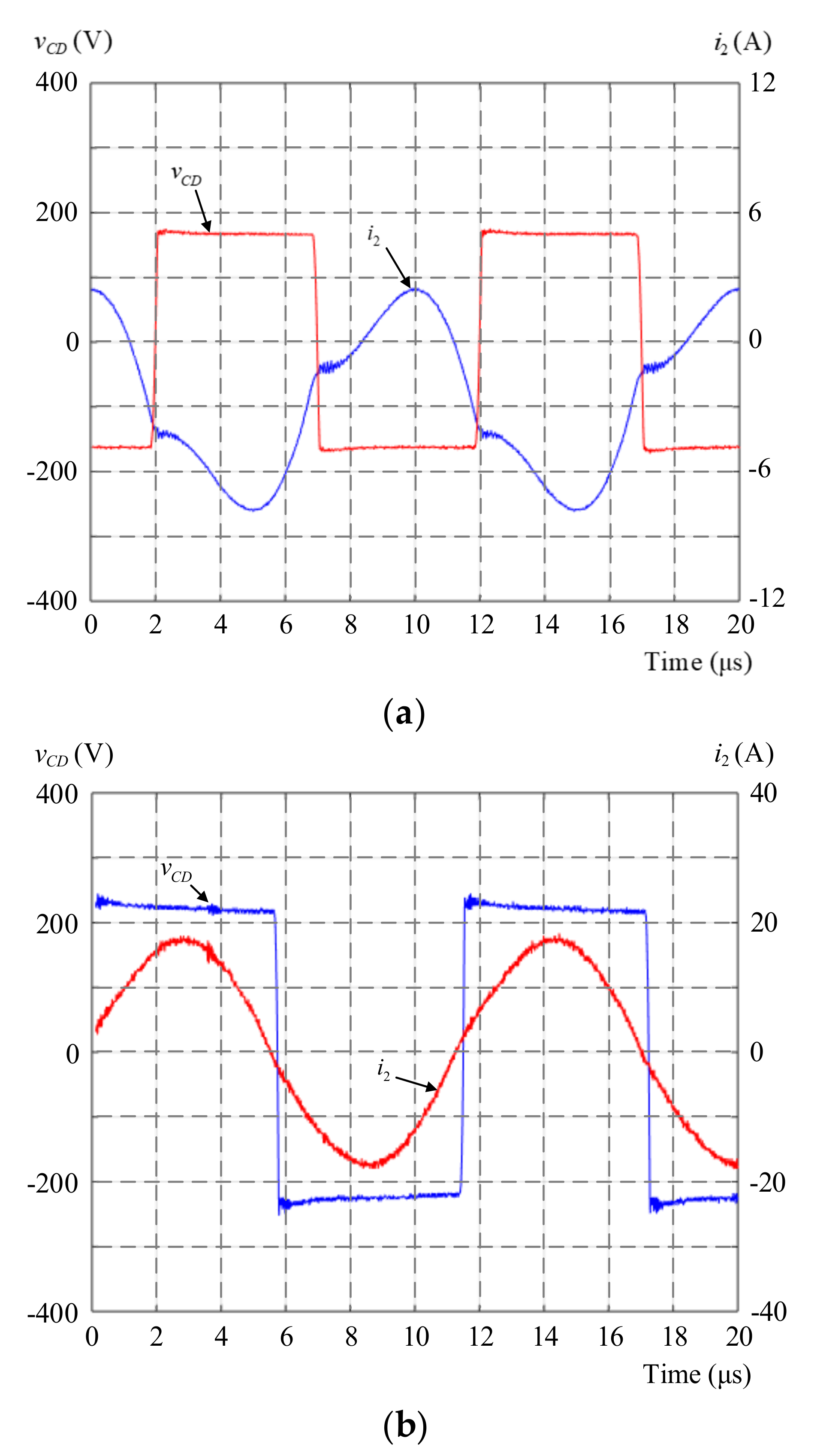
Figure 10a,b show the measured secondary voltage
and secondary current
at 200 W and 2 kW. The secondary current
is closer to a sinusoidal waveform as the output power is increased to 2 kW.
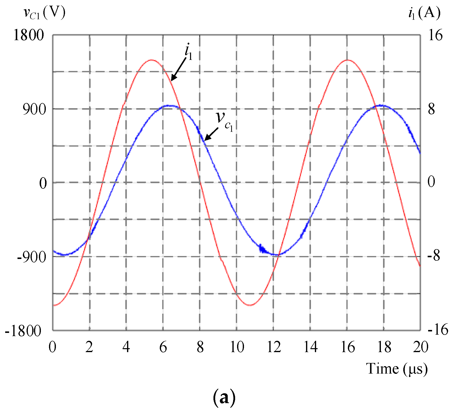
Figure 11a,b show the measured voltages across the primary compensating capacitor
and the secondary compensating capacitor
at 200 W and 2 kW. Both of the
and
are near sinusoidal waveforms. In addition, the amplitude of
reaches 800 V, and the amplitude of
reaches 1300 V at 2 kW. It can be observed that high-stress capacitors should be used for
and
in this proposed IPT system.
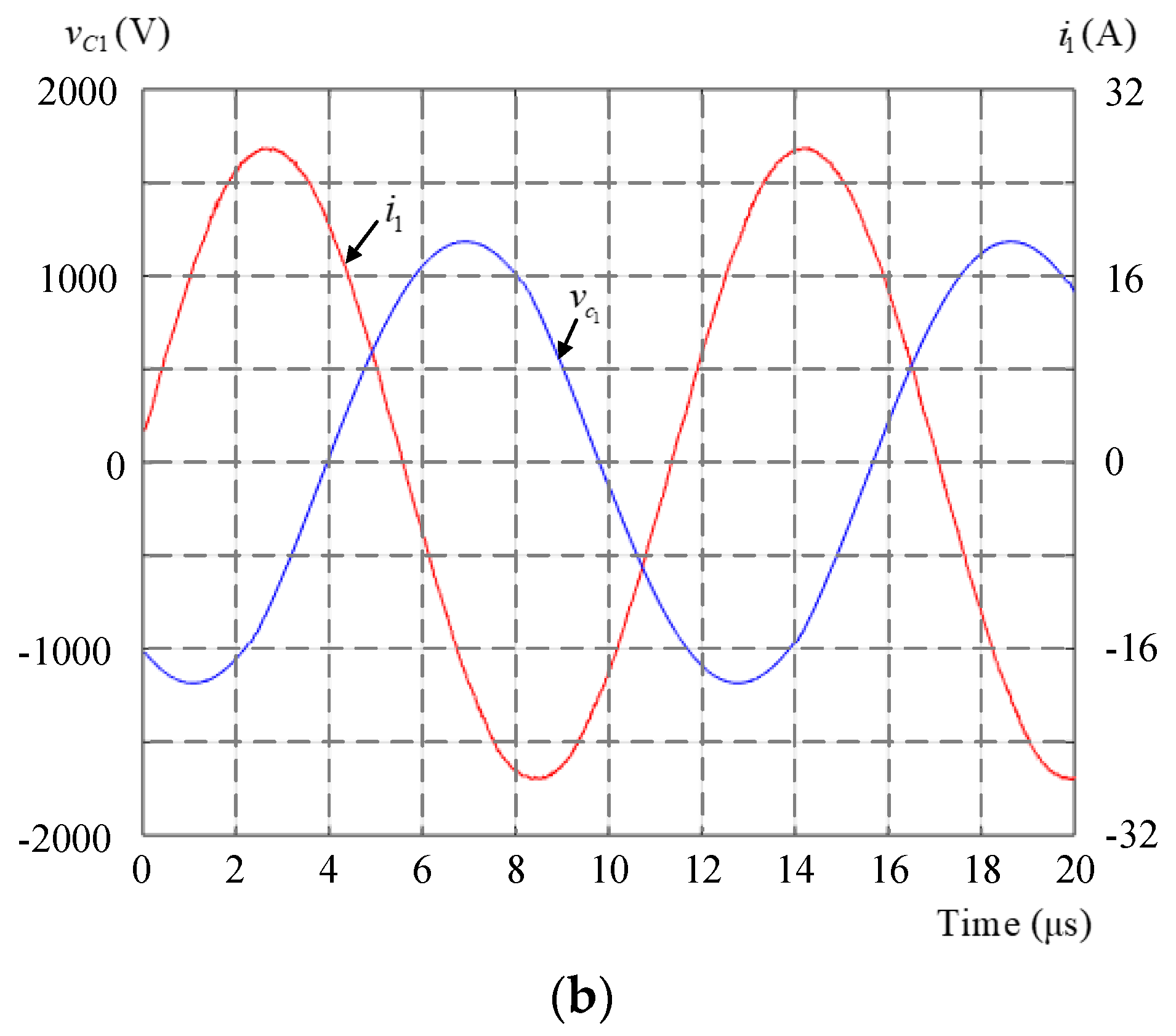
Figure 12a shows the measured third winding current
and its compensation capacitor voltage
at 200 W, in which the phase difference between
and
is near 25° at a light load.
Figure 12b shows the measured third winding current
and its compensation capacitor voltage
at 2 kW, in which the phase difference between
and
is near 90° due to the heavy output load. The reason is that the third winding only has inductance and capacitance without any resistance.
Figure 13a,b show the measured output voltage at 200 W and 2 kW. The output inductor current
is increased from 1.5 A to 13 A as the output power is increased from 200 W to 2 kW. In addition, the inductance current has obvious ringings at 2 kW. The main reason is that a heavy load creates more store energy in the inductance, which creates more ringings when the power switch is turned on or off. The output voltage, however, is very smooth since a large capacitance is used in this paper. Due to the high-frequency operation of the IPT, the reactances of the leakage inductances can be canceled by the reactances of the capacitors. As a result, the input power in the primary winding can be effectively transferred to the output power in the secondary winding.
From
Figure 14a,b,
Figure 15a,b and
Figure 16a,b, we can see the dynamic performance of the proposed IPT.
Figure 14a shows the measured output voltage responses during transient responses. The predictive controllers provide a lower overshoot than PI controllers. In addition, a smaller weight factor can provide lower overshoot response because the control input of the IPT system can increase the current, which creates more energy. Taking
Figure 14a as an example, from 0
to 1
, the performance index
shown in Equation (41) is 1.5 for the weighting factor
=0.1, and the performance index
becomes 2.3 for the weighting factor
=0.3. The performance index can be calculated by using voltage error, control input
, weighting factor
, and a time interval.
Figure 14b shows the measured output voltage responses during load disturbance. An external load of 4 A is added at 20
ms. A smaller weight factor provides a quicker recovery response again.
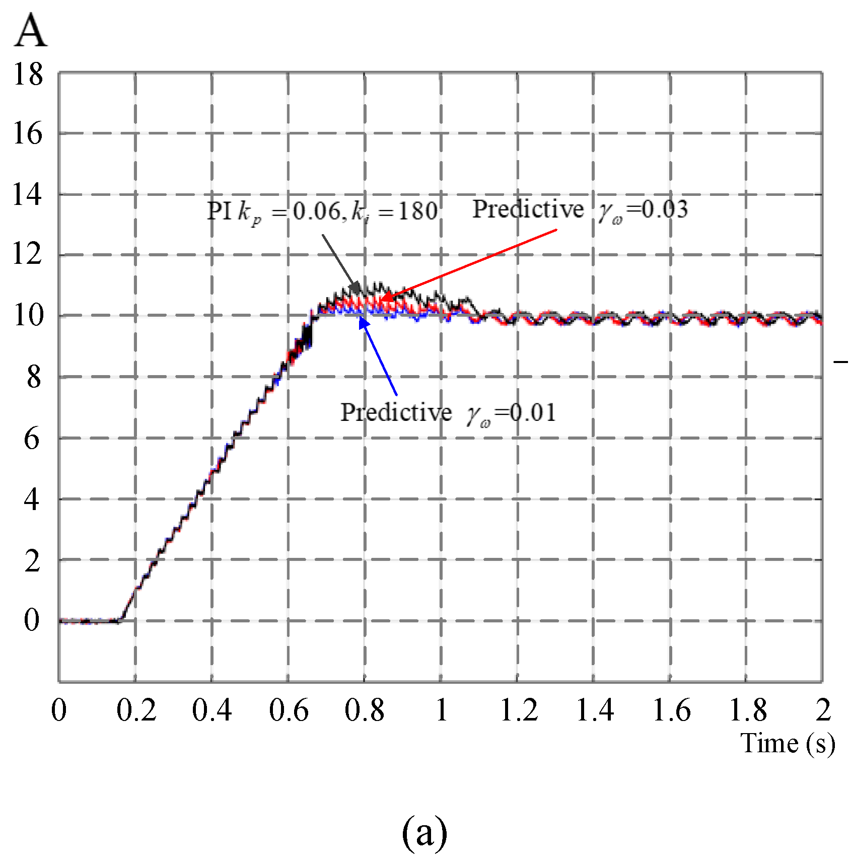
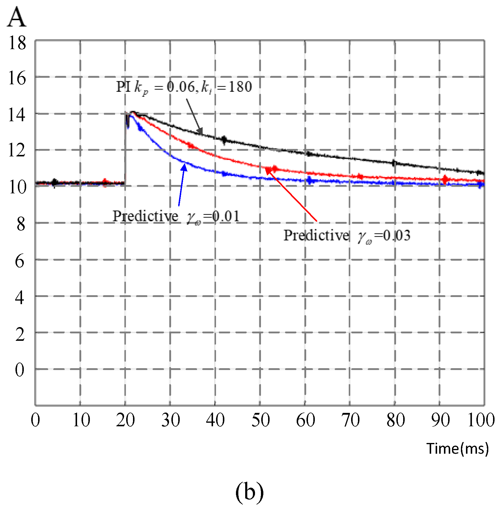
Figure 15a shows the measured output current transient responses, and
Figure 15b shows the load disturbance responses of the output currents. The predictive controllers provide faster recovery times than the PI controllers. In addition, a smaller weight factor can provide a quicker response because the control input of the IPT system can increase the current, which creates more energy.
Figure 16 shows the measured battery voltage and its charging current by using the proposed IPT system. The battery is charged using a constant current at the beginning and then is charged using a constant voltage. The largest charging current is set as 15 A due to the limitation of the battery. However, when the required current charging time is reached, the charging is gradually reduced to 1 A.
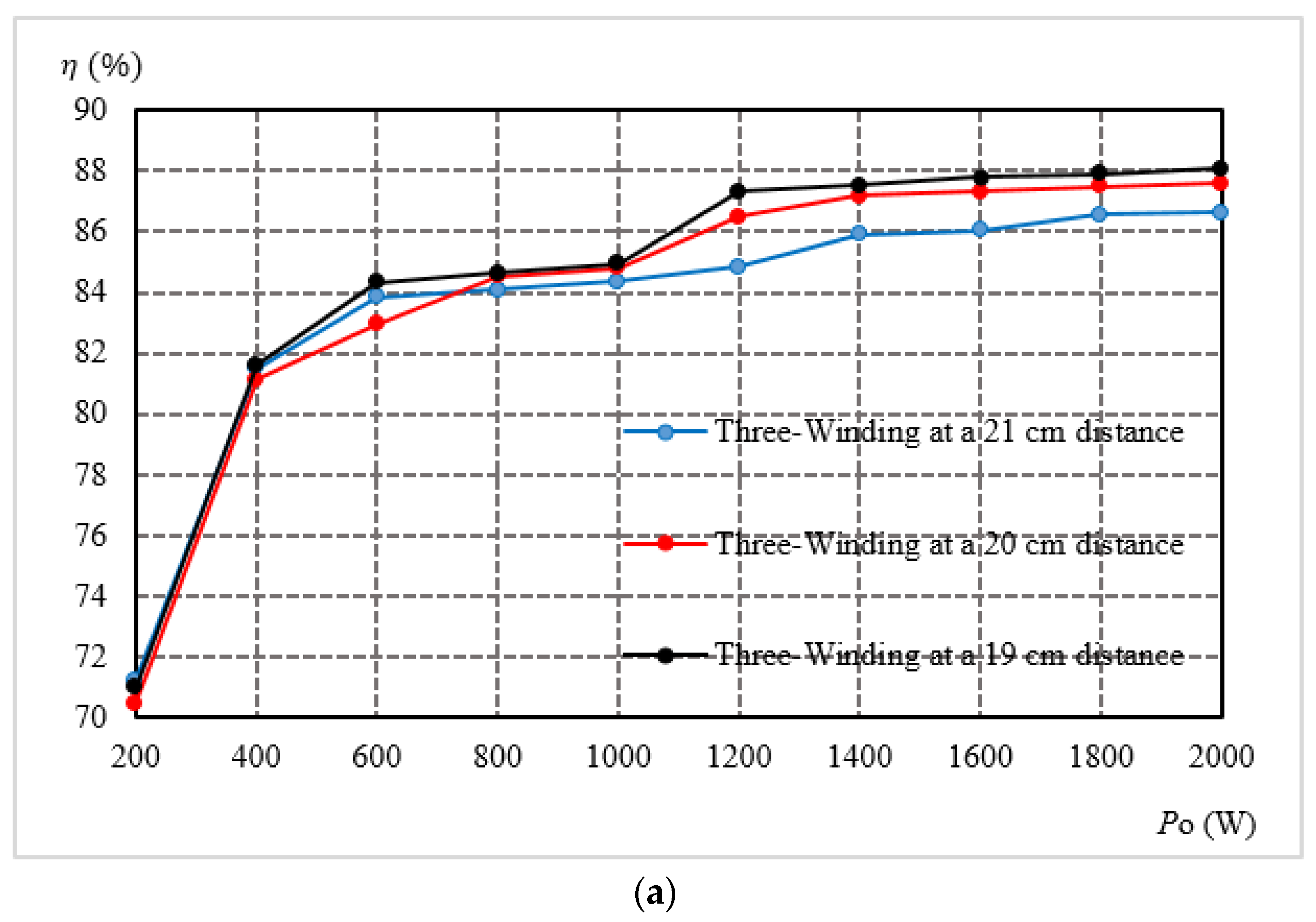
Figure 17a demonstrates the measured efficiency of the three-winding IPT at different distances between the primary winding and secondary winding. From
Figure 17a, the shortest distance provides the highest efficiency for the IPT system. In addition, with a 20 cm air gap, the IPT system reaches 88% efficiency at a 2kW output. However, when the air gap increases, the efficiency of the IPT decreases.
Figure 17b demonstrates the measured efficiency of the three-winding IPT with different misalignments. From
Figure 17b, the shortest misalignment, which is 0 cm, provides the highest efficiency for the IPT. The operations of the IPT system in misaligned conditions are considered with the same model, but this misalignment could lead to changes in the mutual inductance between the windings and the assumptions made in
Section 1. This issue is very complex; as a result, the paper cannot provide a detailed analysis. Only experimental results are demonstrated in this paper.


