Fault Diagnosis of Transformer Windings Based on Decision Tree and Fully Connected Neural Network

Abstract

While frequency response analysis (FRA) is a well matured technique widely used by current industry practice to detect the mechanical integrity of power transformers, interpretation of FRA signatures is still challenging, regardless of the research efforts in this area. This paper presents a method for reliable quantitative and qualitative analysis to the transformer FRA signatures based on a decision tree classification model and a fully connected neural network. Several levels of different six fault types are obtained using a lumped parameter-based transformer model. Results show that the proposed model performs well in the training and the validation stages, and is of good generalization ability.

1. Introduction

Frequency response analysis (FRA) has been widely used to diagnose the winding and core deformation of power transformers [1]. The main shortcoming of this technique is the inconsistency in analyzing its results as so far, there is no widely accepted code for FRA interpretation. This has motivated researchers to come up with new interpretation techniques such as image processing-based methods [2,3,4,5,6,7,8,9]. For instance, three image features are extracted from the FRA polar plot for fault identification and quantification [2,3,4,5,6]. However, the presented method lacks intelligence and depends on subjective judgement. In [7,8,9], a digital image processing method has also been used to extract 6 texture analysis features, but this technique is not very accurate in quantifying fault level. Morphological image processing method is used to diagnose the power transformer fault types in [8,9], however, this method has a reduced detection accuracy.

The applications of intelligent algorithms such as decision tree, support vector machine, and artificial neural network (ANN) can improve the accuracy of fault diagnosis due to their ability to reduce the error caused by subjective judgment [10,11,12,13,14]. In [15], the variation of frequency response signatures with the fault level and type has been investigated through experimental analysis and particle swarm optimization (PSO). ANN is used in [16] to detect the variation in the resonance frequencies in the FRA signatures.

Various methods were used to interpret FRA data in references [2,3,4,5,6,7,8,9,10,11,12,13,14,15,16,17,18,19,20,21], and the process can be divided into feature extraction and model building. In the selection of feature extraction methods, image processing technology is mentioned in most references. For example, the paper [4] extracted graphics parameters from an FRA polar map, and [7,8,9] extracted features through texture analysis. In fact, when using image processing technology to quantify the FRA curve, we can not only get more and richer features, but also focus on extracting the main features while ignoring the secondary features. In reference [15], the frequency response method is extended to the power transformer with triangle connection. A novel image processing method, feature extraction method, and ensemble learning algorithm for transformer diagnosis are proposed in references [16,17]. References [18,19] give the specific research results of the wind axial displacement and the wind inter turn fault, respectively. All of the above show the trend of deeper mining of frequency response data. Decision trees and SVM (Support Vector Machines) are the most common in the model building. Among them, decision trees are often for its strong generalization ability, fast fitting, and convenient pruning. At present, many methods have been proposed to solve the problem of transformer winding fault diagnosis by using frequency response analysis, but the judgment of fault degree is slightly insufficient. The reason is that the determination of the degree of winding fault requires more comprehensive and detailed feature extraction of FRA data, which also requires higher learning ability of the model. As far as the degree of transformer winding fault is concerned, reference [5] found through experiments that as the fault intensifies, the frequency response curve will shift in a certain trend, and this shift eventually leads to the change of the extracted characteristic value. Reference [22] is also based on experiments, and gives the trend and range of change of graphics parameters for the winding deformation under various fault conditions. FRA feature quantization method that uses the method of calculating Euclidean distance according to frequency band distribution to extract features are proposed in reference [23]. Although it is proved that this method has higher linearity than the feature extraction method of reference [24], it does not give a specific diagnosis method of transformer degree, as it is a calculation method of linear correlation coefficient used in frequency response winding deformation analysis.

This paper is aimed at presenting a new FRA interpretation technique based on decision tree and fully connected neural network, which features high accuracy and easy implementation. Image processing technology is used to process the frequency response curve. High-dimensional features are extracted by methods such as grayscale, image enhancement, image sampling, and projection. Part of the sample of high-dimensional features is divided into training, and part is used for validation, which is used to prove the stability and generalization ability of the model. By comparing with the algorithms provided in the existing literature, it is shows that the proposed algorithm has higher accuracy. Compared with the existing literature, the feature quantization method proposed in this paper can mine FRA data in a deeper level, and the proposed fault type and degree diagnosis algorithm is combined, which has more powerful learning ability and generalization ability. Compared with the judgment of fault degree, which is less studied, this paper provides a feasible scheme, which is proved by simulation.

2. Transformer Simulation Model

2.1. Frequency Response Analysis

The principle of transformer FRA signature measurement is shown in Figure 1. A sweep signal of low amplitude and wide frequency range is injected into the common point of the star-connected winding while the response is measured at the other terminal of each phase. For Δ-connected winding, the measurement setup is a bit deferent [25].

It is shown in Figure 2. When the windings are Y-connected, the frequency response data of the three windings can be measured by the sweep signal from the center point. For Δ-connection, the sweep signal needs to be input twice. When connected to signal input1, the data of output1 and output2 can be measured. When connected to signal input2, the data of output3 can be measured.

As staging actual faults on a real transformer is impractical, researchers implemented their technique on either custom-made transformer models or used simulation models. Lumped parameter model that comprises cascaded series inductors (L) and capacitors (K) and shunt capacitors (C), as shown in Figure 3, is a commonly used simulation model for transformer windings. The winding resistance of transformer is very small. Especially when the scanning frequency is above 1 kHz, the resistance effect can be ignored relative to the inductance and capacitance. The fault simulation method in this paper refers to [26]. The transfer function (TF) of each phase (in dB) is calculated from:

$$dB={\log }_{20}\frac{U_o}{U_i}$$

(1)

where $U_i$ and $U_o$ are input and corresponding output voltages at a particular frequency point. The conventional FRA signature (magnitude and phase) for such a model is as shown in Figure 4.

2.2. Frequency Response Analysis

Different transformer fault type and level are simulated by changing the values of lumped parameter model. The method of changing the component parameter value to simulate each fault is shown in

Table 1. Method of fault simulation.

Fault Type	Component
	C	K	L
Short circuit between turns	/	Increase	Decrease
Broken coil	/	/	Increase
Metal foreign body	/	Increase	/
Axial displacement	Decrease	Decrease	/
Radial inward twist	Increase	/	Decrease
Radial outward twist	Decrease	/	Increase

.

The training set consists of 55 samples, whose fault level contain 10%, 20%, 30%, fault location contain disk 1, 4, 7, and all fault type above are included. The validation set consists of 30 samples, whose fault level range from 5% to 30%, fault location ranges from disk 1 to 7, and also all fault types are included. Furthermore, the number of samples for each failure is equal, regardless of the training set and the validation set. Considering the generalization condition, the fault level in the validation set is chosen randomly. Validation sets are shown in

Table 2. Validation sets.

Type	Location	Level
Short circuit between turns	Disk 1	15%
Short circuit between turns	Disk 3	15%
Short circuit between turns	Disk 4	15%
……
Radial outward twist	Disk 4	29%
Radial outward twist	Disk 6	25%
Radial outward twist	Disk 7	11%

.

2.3. Frequency Response Analysis

In order to enhance the accuracy of the proposed method, the frequency range of the FRA signature is divided into 3 frequency bands, as below:

Frequency band 1: Includes the frequency range 0 kHz to 55 kHz of frequency- amplitude data.

Frequency band 2: Includes the frequency range 15 kHz to 250 kHz of frequency- amplitude data.

Frequency band 3: Includes the frequency range 0 kHz to 250 kHz of phase- amplitude data.

All data sets are divided into 3 groups based on the above frequency ranges and are saved as images for further analysis using digital image processing.

3. Quantification of FRA Signature

Reasonable quantification of FRA signature is a prerequisite for intelligent and high-precision fault diagnosis, so more specific features are needed.

The quantification method in this paper is divided into two steps, namely, preprocessing and curve image projection as per the flowchart in Figure 5.

3.1. Preprocessing

All operations in preprocessing are to make sure that the data can be quantified correctly in the curve image projection step, which included image grayscale, segmentation, enhancement, etc. The preprocessing step is aimed at expanding the optional threshold range and resizing all images to 521 × 1992 pixel, to make sure the same quantification standards for all images.

After reading three band images of a sample, graying, image segmentation, and image enhancement are performed in turn. Graying the image is more convenient for line operation of the curve image. Image segmentation preserves part of the curve information and eliminates the interference of the coordinate axis. The enhanced image has higher contrast, which can reach the range of threshold selection in curve image projection.

The curve images of three frequency bands are resized to 521 × 664 after the above processing. In order to represent the samples in the form of images, the three band images are merged horizontally, and the combined image size is 521 × 1992.

3.2. Curve Image Processing

The core operation of curve image projection is column projection. This operation aims to reduce the dimension of curve image to vector. Firstly, a threshold is selected to distinguish curve information from background information. Then, the case column facilitates the whole image, and the number of rows containing curve information is retained in the vector as the element value. After traversal, a 1992 dimensional vector will be generated to express the characteristics of frequency response curve.

Project by column after preprocessing guarantees that all dimensions of the projection vector and the range of vectors value are the same. In this paper, all the vectors’ dimensions are 1992 and the vectors’ value ranges from 0 to 512.

To show the original appearance of the curve images, process vectors’ values by formula below:

$$V(i)=r-v(i)$$

(2)

$V\left(i\right)$, $v\left(i\right)$ represent the vectors processed before and after, respectively.

3.3. Feature Vector

The vector above can reflect the original appearance of the curve image. In order to amplify the difference information, the feature vector is obtained by subtracting the normal sample vector from all vectors.

The obtained feature vector not only reflects the curve difference between the fault sample and the normal condition, but also the appearance of some element value with small scale promoted the choosing of features and the training of models.

4. Fault Diagnosis and Algorithm Comparison

4.1. Fault Type Diagnosis

The distribution of the feature vectors of the training set samples with different fault types is shown in Figure 6. In frequency band 1, each fault type presents a positive and negative alternate state. In frequency band 2, there is a high consistency between the broken coil and the radial outward twist in the first half, while the axial displacement and the radial inward twist in the second half are highly consistent. Each fault type in band 3 has unique distribution characteristics.

4.1.1. Decision Tree Classification Model

Decision tree is a classic machine learning algorithm. As a base learner of ensemble algorithms, its learning ability is not outstanding, but it is famous for its high generalization ability and feature filtering ability.

Decision tree is a hierarchical structure that continuously iterates on features with high impurity. With the increase in the number of iterations, the model is trained more and more exhaustively. The model training is stopped by controlling hyperparameters such as the number of selected features, the maximum depth of the tree, and the minimum sample size of branches [14,15,16,17,18,19,20,21,22,23,24,25,26].

4.1.2. Model Adjustment

The adjustable parameters of the decision tree model include the impurity index, maximum depth of the decision tree, maximum number of selected features, and the minimum number of samples. Among them, the impurity index and the maximum depth of the tree have the greatest impact on the model, while the minimum number of samples in the branch varies with the data sets.

Although as the depth increases, the model will learn more detailed data, but it also leads to a decrease in the generalization ability, which causes the model to perform poorly on the validation stage. The maximum depth of the model is set to 10, and the minimum sample size of the selected branch is set to 9 in this paper.

Gini coefficient is chosen to represent the impurity index. The five feature contributions with the highest Gini coefficients selected by the decision tree are shown in Figure 7. The features selected by the model only account for 0.25% of the all features, so the generalization ability of the model is strong.

4.1.3. Model Effect

The accuracy and generalization ability of the model are tested with the training set and the validation set, and the results are shown in Figure 8. It can be concluded from the result that the model performs well in both data sets. All of the fault type in training set are distinguished correctly, and the accuracy in the validation stage is 96.67%. The high-precision performance in the training set and the validation set shows that the decision tree classification model has strong generalization ability.

4.1.4. Analysis of Frequency Response Curve Using Model

The mentioned decision tree classification model performs well on the data set. The 5 features with the highest contribution 5 extracted by this model: 18, 26, 701, 1279, and 1395. Among them, the 18th and 26th features are located in the place where the numerical value changes in Band 1 are relatively gentle; 701 and 1279 are located at the beginning and end of Band 2. It is worth noting that they are not at the extreme point. The 1395th feature is located in Band 3, which is also where the amplitude changes relatively smoothly.

There is one characteristic among the above features. That is, although these characteristics will change with different faults, they are not extreme points, and the amplitude is much smaller than that of the extreme points. This shows that the extreme point information has its special characteristic’s physical meaning, but may not be the best feature for fault classification. Although the features selected by the decision tree classification model are common, they can reflect the characteristics of various types of faults based on data to a certain extent.

4.2. Fault Level Diagnosis

The distribution of the feature vectors of the training set with different fault levels is shown in Figure 9. The eigenvector exhibits an increase in the amplitude in Band 1 and the distribution of extreme points in Band 2. As the fault level increases, the lower extreme points have a tendency to move to the boundary of Band 2. Band 3 shows a more chaotic distribution characteristic.

4.2.1. Fully Connected Neural Network

Compared with the machine learning algorithm, the deep learning algorithm of the neural network model has a stronger learning ability. In the face of high-dimensional feature samples, the regression ability has a higher limit than that of machine learning [20,21,22,23,24,25,26,27,28,29,30,31,32,33,34]. However, more hyperparameters make it difficult to fit the data, and it’s easier to over fitting during training. Fully connected neural network is shown in Figure 10. The model contains 35 neurons in a single layer, ReLU is chosen to be the activation function.

As we all know, the principle of the neural network model is gradient descent principle. Many iterations on the loss function make the model have strong learning ability, but it also means that the generalization ability of the model is not necessarily good. Therefore, this paper sets up Dropout layer and L2 Regularization, two small tricks to suppress the overfitting phenomenon.

4.2.2. Hyperparameters Setting

The selection of the hyperparameter affects the model performance, which includes regularization method and parameters, abandonment rate of dropout layers, epochs, and callbacks, etc.

The more epochs, the more likely the model is to learn more specifically. The callbacks adjust the learning rate during the training process according to the learning curve of the validation set, which will slow down the fitting speed and reduce the risk of over fitting.

In order to ensure the generalization ability of the model, set a callback function, when the loss function of the validation set does not decrease within 30 epochs, the learning rate will be halved, and due to the setting of the callbacks, epochs should be set larger.

In this paper, the L2 regularization is selected as the penalty term to reduce the complexity of the model to suppress overfitting. Combined with the Mean Square Error (MSE) loss function, the whole loss function in this paper is:

$$loss=\frac{1}{n}{\displaystyle \sum _{i=1}^n(y_{real}-y_{pre})+\lambda \sqrt{{\displaystyle \sum _{i=1}^n{\omega }_i}}}$$

(3)

n, y_real, y_pre, ${\omega }_i$ represent the dimension of feature vector, predict value, real value, and each feature’s weight. The first half of the formula is MSE loss function, and the second half is the regularization term, and λ represents the coefficient of regularization. With the training process progressing, the model weights coefficient is increasing and the generalization ability is decreasing. After the L2 regularization term is added, the model complexity is reduced by penalizing the weight coefficient and the generalization ability of the model is improved.

Dropout layer is also a way to suppress overfitting. The Dropout between the hidden layer and output layer can select a certain proportion of neurons randomly to make them no longer connected to the output layer, which will make the model more difficult to train, and lead to the model having a stronger generalization ability. This method is the same as all the methods of suppressing overfitting, which enhances the generalization ability of the model by slightly sacrificing the fitting effect on the training set.

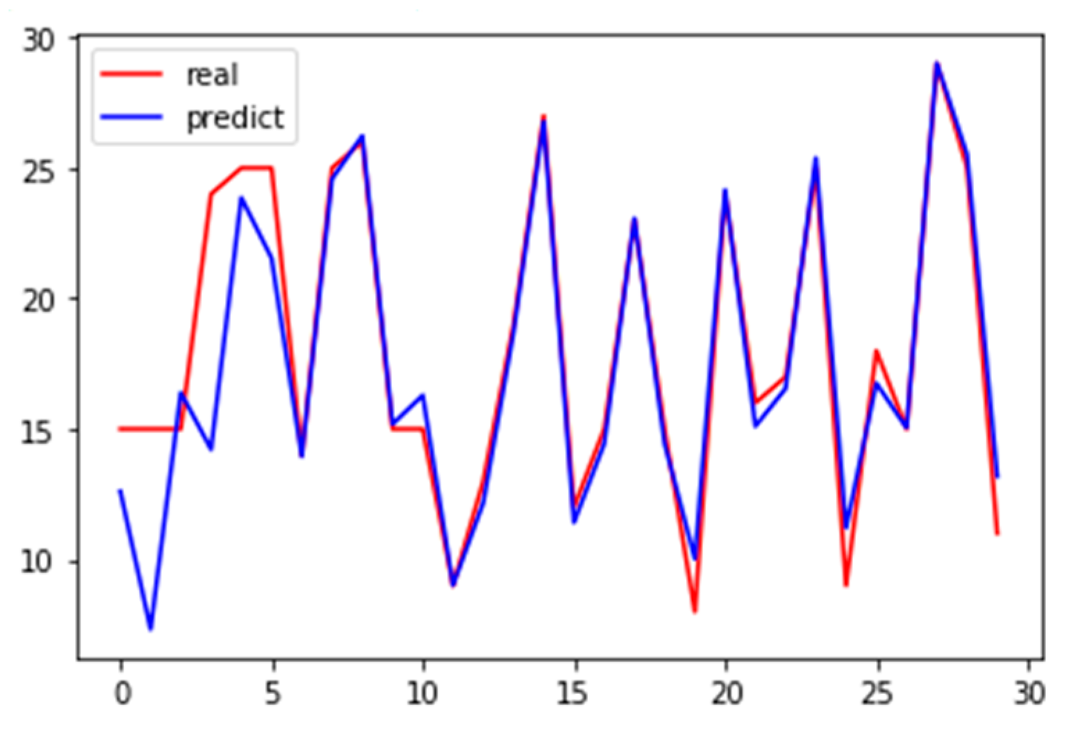
4.2.3. Model Effect and Regressor Explanation

The learning curve of the proposed model is shown in Figure 10, which can show the change of the diagnostic ability of the model in the iterative process and whether there is an overfitting phenomenon. The performance results on the validation set are shown in Figure 11.

It can be seen in Figure 12 that the model is stable, and both Mean Absolute Error (MAE) and MSE on the data set are at a low level. When epochs up to 600, the model are stable basically. It can be seen in Figure 12 that the real value and predicted value are very close, which means that the model is highly accurate and not overfitted.

Figure 11 shows the results of the fully connected layer network model on the verification set. The majority of fault levels are diagnosed precisely except for a few samples. The MAE and MSE of the validation set are 1.3764 and 6.5316, respectively.

The above-mentioned MAE and MSE for all fault types are 1.3756 and 6.5316, respectively. In order to understand the fault level diagnosis effect of the regression model for various fault types more specifically, the maximum and minimum predict deviations, MAE and MSE, between the model diagnosis results and the real value under each fault type are calculated, respectively. The results are shown in

Table 3. Performance of regression model under each fault type. MAE: Mean Absolute Error; MSE: Mean Square Error.

Fault Type	Maximum Predict Deviation/%	Minimum Predict Deviations/%	MAE	MSE
Radial outward twist	9.7833	1.1385	4.4752	32.7039
Radial inward twist	3.4548	0.0578	0.8687	2.44
Axial displacement	1.2944	0.0076	0.53	0.5016
Metal foreign body	2.0251	0.0762	0.7639	1.0183
Broken coil	2.2046	0.1674	0.8203	1.2079
Short circuit between turns	2.1844	0.0172	0.8001	1.3177

. The fitted curve is shown in Figure 13.

It can be observed from Table 3 that the proposed model has the highest diagnostic accuracy for Axial displacement and the worst diagnostic effect for Radial outward twist. The difference between their MAE and MSE is 8 times and 64 times, respectively. The accuracy of the proposed model for the remaining 4 fault types is similar. We can observe more specifically from the fitting curve in Figure 13 that the reason causes the high MAE and MSE of the Radial outward twist is that the prediction deviations of the three samples under the fault are small, while the prediction deviations of sample 1 and sample 4 are large, especially sample 4, which is up to 9.7833%.

In the case of radial outward twist fault, the second and fourth samples of the test set are quite different from the real value. The reason for the deviation is that the training set sample size is small when realizing the dual diagnosis of fault grade and type, which will lead to a low upper limit of the generalization ability of the model. When the two variables of fault type and fault degree change at the same time, more fault samples are needed to train the model.

4.3. Algorithm Comparison

Intelligent diagnosis of transformer winding fault types has been realized since the artificial intelligence algorithms were introduced. However, the diagnostic accuracy varies with the feature extraction method and classification algorithm. As far as diagnosis accuracy is concerned, intelligent algorithms are not the only influencing factor. Different feature extraction methods will also affect the subsequent diagnosis accuracy directly. The excellent feature extraction algorithms can fully contain or reflect the characteristics of the curve while ignoring trivial and unimportant features. The more detailed and concise the extracted features, the better the effect of model learning.

4.3.1. Fault Type Diagnosis Comparison

In [21], three types of faults: DSV (disk space variation), SC (inter-disk short circuit), and RD (radial deformation) are discussed. The frequency response data set are based on actual measurement results, and has a richer sample size than this paper. The differences between the faults are also more obvious than this paper.

This paper uses the feature extraction method and PSO-SVM model, which was used in [21] to train and classify our data set. After training the model on the training set, the result of the validation set is as shown in Figure 14.

As shown in Figure 12. The accuracy of the model on the validation set only up to 76.67%, which is far below the decision tree model of this paper. In fact, decision trees and SVM are both very successful machine learning models, but the low accuracy is attributed to the feature extraction methods. The 8 features are obtained based on global performance of data are not full enough to represent the FRA data, so that the SVM cannot get enough information to classify the different samples.

4.3.2. Fault Level Diagnosis Comparison

PSO-SVM regressor model is used in [20] to quantify fault levels. The performance of the trained model in the training set is shown in Figure 15. It can be observed from Figure 15 that the performance of the PSO-SVM model on the validation set is poor. For a more specific comparison, MAE and MSE on the data set are calculated as shown in

Table 4. MAE and MSE of the model on the data set.

	MAE	MSE
Train	3.5820	18.2164
Test	7.1396	72.6370

. The MAE and MSE of PSO-SVM training data are even higher than the validation data of a fully connected neural network, which also shows that the SVM don’t get enough information from features. On the other hand, the model for fault level diagnosis has an obvious overfitting phenomenon in the training set and test set in [20], which may prove that PSO may not be a powerful enough optimization algorithm for SVM model.

All in all, adequate quantitative algorithms and deep learning networks with more powerful learning capabilities are the reasons for the better performance of the model.

5. Conclusions

In order to extract FRA data features deeply, a curve image feature extraction method based on image processing technology is proposed in this paper. This method filters the FRA data and uses the projection method to obtain high-dimensional feature vectors that can reflect the full curve of the data. These feature vectors can obtain very high-precision diagnosis results when used in the decision tree model to diagnose fault types. At the same time, after training the feature vector with the fully connected neural network model, it can be used to identify the degree of fault.

References

1. Shaban, A.E.; Ibrahim, K.H.; Barakat, T.M. Modeling, Simulation and Classification of Power Transformer Faults Based on FRA Test. In Proceedings of the 2019 21st International Middle East Power Systems Conference (MEPCON), Cairo, Egypt, 17–19 December 2019. [Google Scholar]
2. Aljohani, O.; Abu-Siada, A. Application of Digital Image Processing to Detect Short Circuit Turns in Power Transformers using Frequency Response Analysis. IEEE Trans. Ind. Inform. 2016, 12, 2062–2073. [Google Scholar] [CrossRef]
3. Aljohani, O.; Abu-Siada, A. Application of digital image processing to detect transformer bushing faults and oil degradation using FRA polar plot signature. IEEE Trans. Dielectr. Electr. Insul. 2017, 24, 428–436. [Google Scholar] [CrossRef]
4. Juan, C.; Yang, X.-J. Application of Digital Image Processing to Measurement System of Temperature Field in Molten Pool for Laser Remanufacturing. Appl. Laser 2006, 26, 212–220. [Google Scholar]
5. Aljohani, O.; Abu-Siada, A. Application of DIP to Detect Power Transformers Axial Displacement and Disk Space Variation Using FRA Polar Plot Signature. IEEE Trans. Ind. Inform. 2017, 13, 1794–1805. [Google Scholar] [CrossRef] [Green Version]
6. Abu-Siada, A.; Hashemnia, N.; Islam, S.; Masoum, M.A.S. Understanding power transformer frequency response analysis signatures. IEEE Electr. Insul. Mag. 2013, 29, 48–56. [Google Scholar] [CrossRef]
7. Zhao, X.; Yao, C.; Li, C.; Zhang, C.; Dong, S.; Abu-Siada, A.; Liao, R. Experimental evaluation of detecting power transformer internal faults using FRA polar plot and texture analysis. Int. J. Electr. Power Energy Syst. 2019, 108, 1–8. [Google Scholar] [CrossRef]
8. Xu, Y.; Gong, Y.-P.; Liu, Y.-W.; Ma, W.-Y.; Zhao, Q.; Wang, W.-H. A block frequency analysis method for frequency response data of transformer windings. Autom. Electr. Power Syst. 2014, 38, 91–97. [Google Scholar]
9. Mao, Y.Z.; Wang, W.; Li, D.M.; Yang, Z.L. Application of Morphological Filtering in Noise Reduction of Partial Discharge of Transformer. Transformer 2014, 51, 32–35. [Google Scholar]
10. Sun, Z.; Sun, Z.L.; Wei, J. Research on power transformer fault diagnosis based on decision tree support vector machine algorithm. J. Electr. Eng. 2019, 14, 42–45. [Google Scholar]
11. Liu, P.; Zhang, W. A Fault Diagnosis Intelligent Algorithm Based on Improved BP Neural Network. Int. J. Pattern Recognit. Artif. Intell. 2019, 33, 50–56. [Google Scholar] [CrossRef]
12. Li, Z.-H.; Xiang, X.; Hu, T.-H.; Abu-Siada, A.; Li, Z.; Xu, Y. An improved digital integral algorithm to enhance the measurement accuracy of Rogowski coil-based electronic transformers. Int. J. Electr. Power Energy Syst. 2020, 118, 105806. [Google Scholar] [CrossRef]
13. Zhang, W.; Yang, X.; Deng, Y.; Li, A. An Inspired Machine-Learning Algorithm with a Hybrid Whale Optimization for Power Transformer PHM. Energies 2020, 13, 3143. [Google Scholar] [CrossRef]
14. Liu, J.; Zhao, Z.; Tang, C.; Yao, C.; Li, C.; Islam, S. Classifying Transformer Winding Deformation Fault Types and Degrees using FRA based on Support Vector Machine. IEEE Access 2019, 7, 112494–112504. [Google Scholar] [CrossRef]
15. Banaszak, S.; Kornatowski, E.; Szoka, W. The Influence of the Window Width on FRA Assessment with Numerical Indices. Energies 2021, 14, 362. [Google Scholar] [CrossRef]
16. Duvvury, V.S.B.C.; Pramanik, S. An Attempt to Identify the Faulty Phase in Three-Phase Transformer Windings Using an Advanced FRA Measurement Technique. IEEE Trans. Power Deliv. 2020, 1. [Google Scholar] [CrossRef]
17. Zhang, C.; He, Y.; Du, B.; Yuan, L.; Li, B.; Jiang, S. Transformer fault diagnosis method using IoT based monitoring system and ensemble machine learning—ScienceDirect. Future Gener. Comput. Syst. 2020, 108, 533–545. [Google Scholar] [CrossRef]
18. Sun, A.; Xu, X.; Liu, H.; Wang, K.; Zhou, X. Transformer Winding Fault Analysis Based on Oscillatory Wave Binarization Image Processing. In Proceedings of the 2020 5th Asia Conference on Power and Electrical Engineering (ACPEE), Chengdu, China, 4–7 June 2020. [Google Scholar]
19. Tahir, M.; Tenbohlen, S. FRA lookup charts for the quantitative determination of winding axial displacement fault in power transformers. IET Electr. Power Appl. 2020, 14, 2370–2377. [Google Scholar] [CrossRef]
20. Maraaba, L.S.; Twaha, S.; Memon, A.; Al-Hamouz, Z. Recognition of Stator Winding Inter-Turn Fault in Interior-Mount LSPMSM Using Acoustic Signals. Symmetry 2020, 12, 1370. [Google Scholar] [CrossRef]
21. Zhang, S.; Hu, Q.; Wang, X.; Wang, X.; Wang, D. Research of transformer optimal design modeling and intelligent algorithm. In Proceedings of the 2011 Chinese Control and Decision Conference (CCDC), Mianyang, China, 23–25 May 2011; pp. 213–218. [Google Scholar]
22. Li, Z.; Jiang, W.; Abu-Siada, A.; Li, Z.; Xu, Y.; Liu, S. Research on a Composite Voltage and Current Measurement Device for HVDC Networks. IEEE Trans. Ind. Electron. 2020, 1. [Google Scholar] [CrossRef]
23. Ni, J.; Zhao, Z.; Tan, S.; Chen, Y.; Yao, C.; Tang, C. The actual measurement and analysis of transformer winding deformation fault degrees by FRA using mathematical indicators. Electr. Power Syst. Res. 2020, 184, 106324. [Google Scholar] [CrossRef]
24. Zhang, C.Y.; Hu, H.; Cheng, H.H.; Liu, Y.P.; Xu, K.; Zhang, P.; Zhou, J.X. Diagnosis method of power transformer winding deformation degree and type based on Euclidean distance analysis. High Volt. Appar. 2020, 56, 224–230. [Google Scholar]
25. Cheng, S. The correct application of frequency response correlation coefficient analysis and judgment of winding deformation. High Volt. Appar. 2006, 42, 66–69. [Google Scholar]
26. Cheng, H.-H. Transformer Winding Deformation Diagnosis Based on Frequency Response Complex Values and Gray Projection Method. Master’s Thesis, North China Electric Power University, Beijing, China, 2018. [Google Scholar]
27. Xie, H.; Chen, J.; Zhang, P. Knowledge acquisition method of power transformer condition assessment based on SMOTE and decision tree algorithm. Electr. Power Autom. Equip. 2019, 40, 137–142. [Google Scholar]
28. Menezes, A.G.C.; Almeida, O.M.; Barbosa, F.R. Use of decision tree algorithms to diagnose incipient faults in power transformers. In Proceedings of the 2018 Simposio Brasileiro de Sistemas Eletricos (SBSE), Niteroi, Brazil, 12–16 May 2018; pp. 1–6. [Google Scholar]
29. Li, H.; Li, Z.; Hou, H.; Sheng, G.; Jiang, X.; Hu, J. An Intelligent Transformer Warning Model based on Data-driven Bagging Decision Tree. In Proceedings of the 2018 Condition Monitoring and Diagnosis (CMD), Perth, WA, USA, 23–26 September 2018; pp. 1–5. [Google Scholar]
30. Admasie, S.; Bukhari, S.B.A.; Gush, T.; Haider, R.; Kim, C.H. Intelligent Islanding Detection of Multi-distributed Generation Using Artificial Neural Network Based on Intrinsic Mode Function Feature. J. Mod. Power Syst. Clean Energy 2020, 8, 511–520. [Google Scholar] [CrossRef]
31. Hong, K.; Jin, M.; Huang, H. Transformer winding fault diagnosis using vibration image and deep learning. IEEE Trans. Power Deliv. 2020, 1. [Google Scholar] [CrossRef]
32. Qi, M.; Wang, Y.; He, R.-X. Research on Transformer Fault Diagnosis based on Improved Fuzzy Neural Network. J. Chengdu Technol. Univ. 2019, 22, 43–45. [Google Scholar]
33. Zhu, N.; Liu, C.; Laine, A.F.; Guo, J. Understanding and Modeling Climate Impacts on Photosynthetic Dynamics with FLUXNET Data and Neural Networks. Energies 2020, 13, 1322. [Google Scholar] [CrossRef] [Green Version]
34. Hu, W.; Lu, Z.-X.; Wu, S.-Z.; Zhang, W.; Dong, Y.; Yu, R.; Liu, B. Real-time transient stability assessment in power system based on improved SVM. J. Mod. Power Syst. Clean Energy 2019, 7, 26–37. [Google Scholar] [CrossRef] [Green Version]
Figure 1. FRA (frequency response analysis) measurement for star-connected winding.
Energies 14 01531 g001
Figure 2. Simple schematic diagram of measurement method.
Energies 14 01531 g002
Figure 3. Transformer lumped parameter model.
Energies 14 01531 g003
Figure 4. Conventional FRA signature.
Energies 14 01531 g004
Figure 5. Curve image quantization flowchart.
Energies 14 01531 g005
Figure 6. Feature vectors distribution of different fault types.
Energies 14 01531 g006
Figure 7. Feature contribution.
Energies 14 01531 g007
Figure 8. Classification performance of the model on the data set.
Energies 14 01531 g008
Figure 9. Feature vectors distribution of different fault levels.
Energies 14 01531 g009
Figure 10. Fully connected neural network.
Energies 14 01531 g010
Figure 11. Learning curve.
Energies 14 01531 g011
Figure 12. Performance of the model on validation set.
Energies 14 01531 g012
Figure 13. Model prediction results under various types of failures.
Energies 14 01531 g013
Figure 14. Performance of particle swarm optimization (PSO)-SVM on validation set.
Energies 14 01531 g014
Figure 15. PSO-SVM performance on the data set.
Energies 14 01531 g015