A Study of Developing a Prediction Equation of Electricity Energy Output via Photovoltaic Modules

Abstract

Various equations are being developed and applied to predict photovoltaic (PV) module generation. Currently, quite diverse methods for predicting module generation are available, with most equations showing accuracy with ≤5% error. However, the accuracy can be determined only when the module temperature and the value of irradiation that reaches the module surface are precisely known. The prediction accuracy of outdoor generation is actually extremely low, as the method for predicting outdoor module temperature has extremely low accuracy. The change in module temperature cannot be predicted accurately because of the real-time change of irradiation and air temperature outdoors. Calculations using conventional equations from other studies show a mean error of temperature difference of 4.23 °C. In this study, an equation was developed and verified that can predict the precise module temperature up to 1.64 °C, based on the experimental data obtained after installing an actual outdoor module.

1. Introduction

As the market for photovoltaic modules has increased, studies are being conducted continually to increase the PV module power generation. At the same time, research on PV module power generation prediction has become as important as the research on increasing the efficiency of the PV modules. Most PV modules have a spec mark of PV module power generation in standard test conditions (STC) (25 °C and 1000 W/m²), but actual outdoor installations do not reach this spec. One reason for the failure to reach the spec is irradiation, the factor that has the most influence on PV module power generation. The period during the day when irradiation is maintained at 1000 W/m² is extremely short. In addition, module generation does not satisfy the STC standard of actual air temperature of 25 °C, even if the irradiation was 1000 W/m², because of the internal temperature of the module. Even if the air temperature was 25 °C, the irradiation energy that remains after the PV module power generation increases the module temperature [1,2].

Equations that predict PV module power generation are pretty accurate as long as the values of irradiation and module temperature are accurate. An error range of approximately 1–2% with actual power generation is obtained when based on the equation developed by the Sandia National Laboratory of the United States Department of Energy [3]. When this equation is used, the prediction of PV module power generation can be predicted when the irradiation and the temperature of the PV module are known. However, in reality, research on predicting the temperature of modules is lacking. The performance of the module generation system depends on irradiation, outside temperature, module temperature, and wind speed. It is reported that it is affected by changes in meteorological and environmental conditions. The deterioration of the system performance due to the increase in the PV module temperature should be considered for the accurate performance evaluation of the system as well as the process of calculating the capacity and generation amount of PV module generation system. It has been confirmed that research is needed to evaluate the accuracy and validity of predicting PV module temperature using the prediction model in meteorological conditions [4].

Conventional methods for predicting the temperature of actual modules have the following form [5].

$$T_m =\mathrm{k}\ast I_r+T_A$$

(1)

where

• $T_m$: module temperature (K)
• $\mathrm{k}$: coefficient
• $I_r$: irradiation (W/m²)
• $T_A$: ambient temperature (K)

$$T_{mod}=E\left(e^{a+b\ast WS}\right)+T_{amb}$$

(2)

$$T_{mod}=T_{amb}+H/\left(U_0+ U_1\ast \mathrm{v}\right)$$

(3)

where

• $T_{mod}$: temperature of module [°C]
• $T_{amb}$: temperature of ambient [°C]
• $E, H:$ irradiation [W/m²]
• $a$, b,$U_0, U_1$: coefficient
• WS, $\mathrm{v}$: wind speed [m/s]

In other papers in the same form as Equation (1), equations for predicting temperature have been proposed as Equation (2) [3] and Equation (3) [4].

Regarding Equation (1), coefficients have been suggested by considering variables such as wind speed, outdoor temperature, efficiency, and generation for many predictive models’ module temperature. PV module efficiency is influenced by the insolation, air temperature, wind speed, and relative humidity [6]. The prediction of module temperature with respect to irradiation is convenient when the change of module temperature attains a complete thermal equilibrium, when the air temperature and irradiation are maintained for a certain period. However, this is a continuous phenomenon in outdoor conditions. Irradiation and temperature continuously change in real time in outdoor conditions and the sampling of data has to be conducted in a very short time interval (approximately 30 s to 1 min). The existing equations show a large error in predicting real time changes in the module temperature. When the temperature of the module is predicted through the temperature prediction equation in the same form as in actual Equation (1), the form shown in Figure 1 is shown. The paper shown in Figure 1 is a simulation value using the temperature prediction equation of another paper. The maximum difference in measurements and predictions is up to 9.7 °C.

Therefore, in this paper, an outdoor testbed was established and an equation was developed that can predict module temperature changes in real time.

2. Experimental

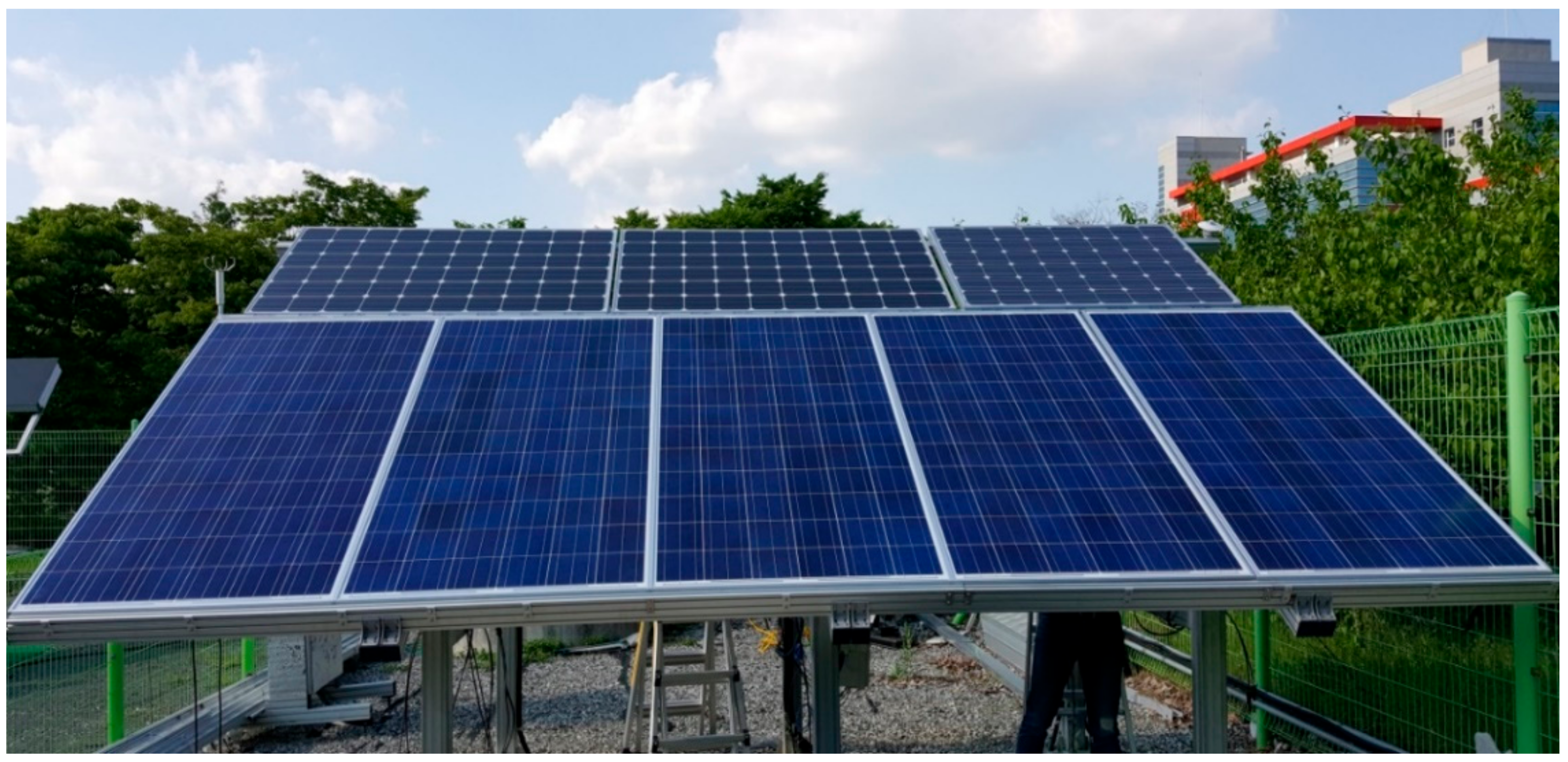
2.1. Outdoor Testbed Setup

As shown in Figure 2, a testbed with fixed modules was established. Up to eight modules can be installed simultaneously in this testbed. The wind direction, irradiation, air temperature, and module temperature were measured, and the data sampling interval was set to 30 s.

The testbed was installed in Gyeongsan-si, South Korea (north latitude 36°), with the installation angle being 30°. An electronic load was used in this study and the maximum power point tracking (MPPT) was continuously traced with an MPPT program. The data-monitoring facility was installed directly adjacent to the test bed and air-conditioned because of the inverter heat. All the data were gathered in the monitoring facility and saved to one server.

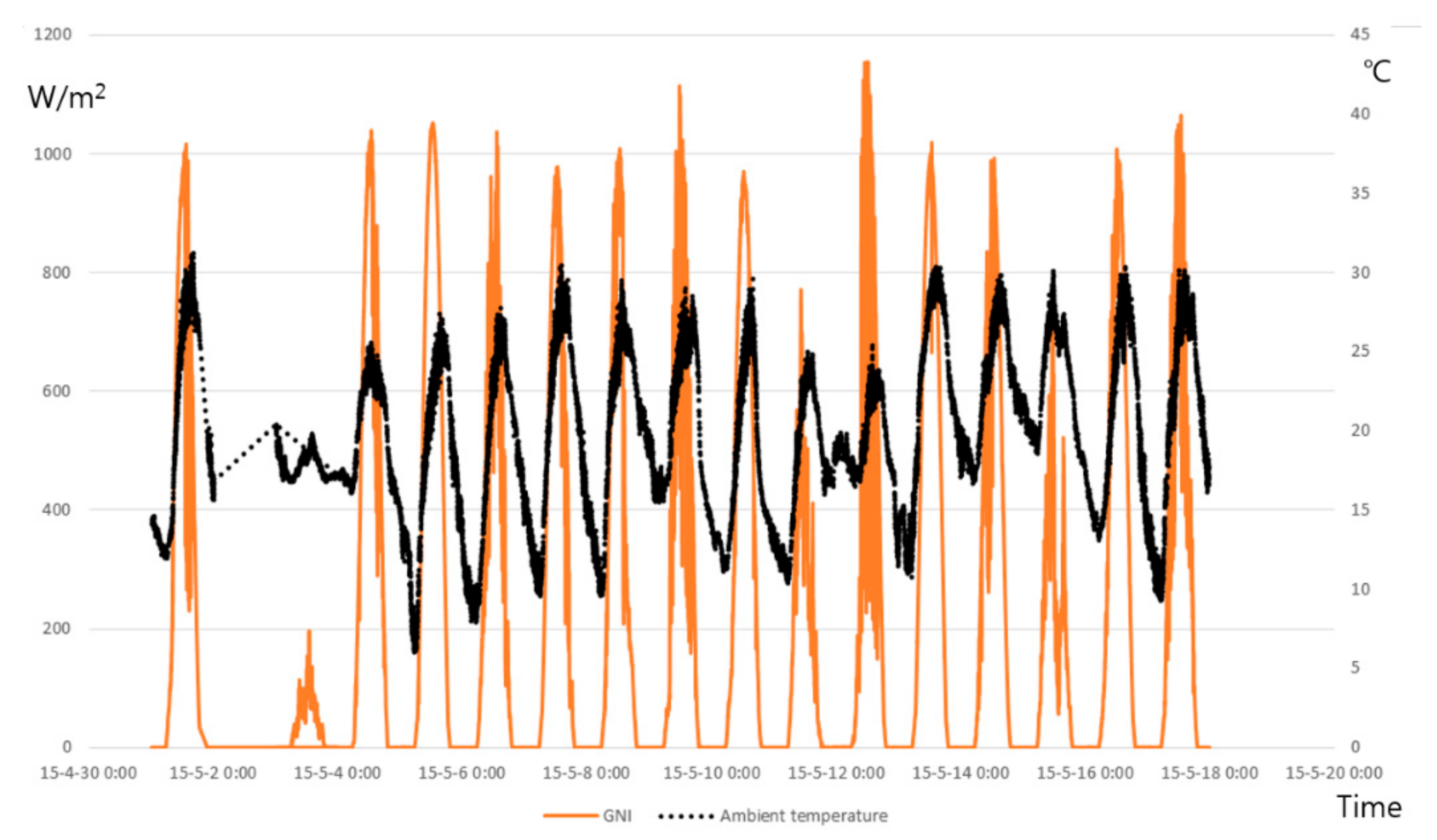
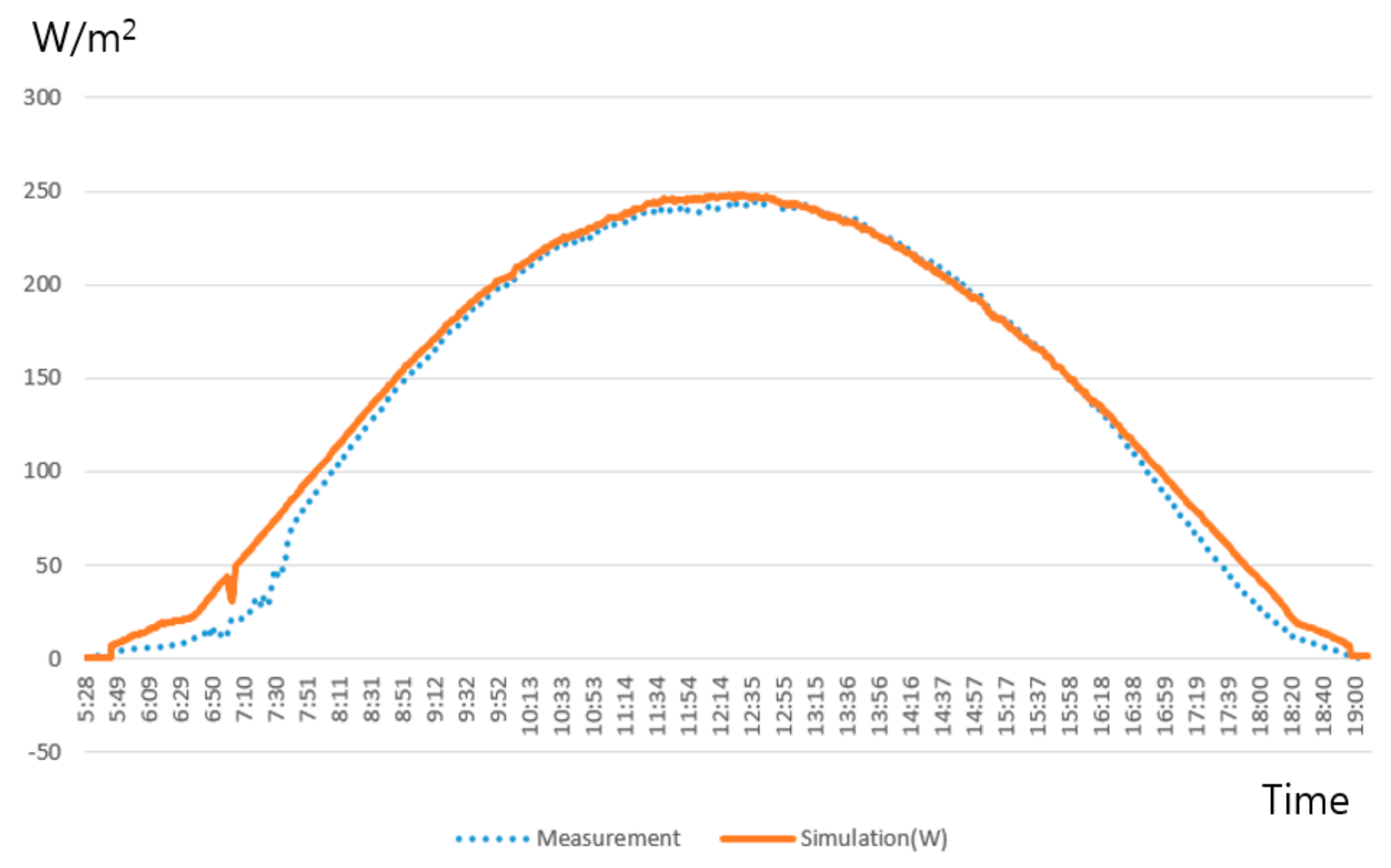
In Figure 3, the x-axis is shown in the order of year, month, day, and hour. The y-axis is two, meaning W/${\mathrm{m}}^2$ and °C. This is a graph obtained by extracting GNI and ambient temperature data for a day. In this experiment, 60 Cell 265 W multi-crystal modules were used. The multi-crystal module size is 1650 mm × 980 mm × 32 mm (including frame). This PV module type is commonly used in solar energy generation at present. The temperature sensor was attached to the center part of the cell, assuming that the temperature distribution on the total module area was actually not large. The actual temperature difference between the center and the corner part of the module was shown to be approximately 1–2 °C [2]. The temperature sensor used a T type sensor and checked the temperature. The model name of the T type is TT-T-24-SLE-1000 and the insulation type has a range of −267 °C to 260 °C for the PFA type. Special Limits of Error is ±0.5 °C or 0.4% and it provides high temperature measurement accuracy. Hence, the testbed was used. In order to increase the accuracy, a weather station was also installed at the MegaWatt (MW) verification development center near Yeungnam University and was used to measure irradiation, ambient temperature, wind speed, wind direction, rainfall, humidity etc. Since both sites showed similar results, the temperature and wind speed data were simulated at the test site for PV modules.

2.2. Outdoor PV Module Temperature Measurement and Modeling

The equation relevant to the module temperature is based on the following equation: [7].

Input = Output + Generation + Accumulation

(4)

where

• Input: irradiation;
• Output: thermal energy emitted from the PV module to the atmosphere;
• Generation: energy generated by the PV module through irradiation;
• Accumulation: input − output − remaining energy after generation.

Input is irradiation; Output is the energy going out to the atmosphere; Generation is the energy that is transmitted after generating electricity; and Accumulation is the remaining energy after the PV module is generated, and it is the remaining energy related to temperature rise. Unlike the previous Equation (1), the decision equation is created. In Equation (4), Output and Generation are Output Energy, and Accumulation is the remaining energy after the module works, so Equation (5) is as follows [7].

Input Energy = Output Energy + Remaining Energy

(5)

where

• Input Energy: irradiation;
• Output Energy: output, going out to the atmosphere + generation;
• Remaining Energy: energy accumulation, after the module works.

It can be deduced from Equation (5) that the energy increasing the module temperature is the remaining energy, which is converted to heat and which subsequently increases the module temperature [5]. Obviously, the heat cannot be measured precisely because the module is not composed of only one material. However, it is assumed that the module is composed of one new integrated material; therefore, the module temperature can be predicted by multiplying the converted value from the remaining energy. The only energy that could enter from the outdoor condition becomes the irradiation. Therefore, the input energy is the irradiation. The output energy is composed of electric energy generated by the module and thermal energy emitted by the difference between the module and the air temperature. The output energy is based on the convective heat transfer Equation (6) by convective energy heat exchange [8].

$$\mathrm{Q} = \mathrm{hA}\Delta \mathrm{T}$$

(6)

where

• $\mathrm{Q}$: convective heat transfer (W);
• $\mathrm{h}$: convective heat transfer coefficient (W/(${\mathrm{m}}^2$K));
• $\mathrm{A}$: area (${\mathrm{m}}^2$);
• $\Delta \mathrm{T}$: temperature difference (K).

The convective heat transfer coefficient and temperature difference are moved to the left side and the remaining right side becomes Equation (6) [8].

$$\mathrm{h}\Delta \mathrm{T}=\frac{Q}{A}$$

(7)

Remaining energy is the Input − Output energy balance. It is assumed that the system (target volume) is PV module based on the energy balance equation of chemical engineering thermodynamics [7,8,9].

$$\frac{d\left(mU\right)}{dt}\left[\right(\mathrm{H}+\frac{1}{2}{u}^2+zg)\dot{m}]=\dot{Q}+\dot{W}$$

(8)

where

• mU: internal energy per unit mass [J/kg];
• H: enthalpy [J];
• u: velocity [m/s];
• z: height from the reference level [m];
• g: gravitational acceleration [m/$s^2$];
• $\dot{m}$: mass flow rate [kg/s];
• $\dot{Q }$: heat energy per hour [J/s];
• $\dot{W }$: work rate [J/s].

If Equation (8) is expressed as remaining energy, which is equal to Input − Output and is expressed as Equation (9)

$$\frac{d\left(mU\right)}{dt}=\dot{Q}+\dot{W}-\Delta \left[\right(\mathrm{H}+\frac{1}{2}{u}^2+zg\left)\dot{m}\right]$$

(9)

The Equation (7) left term is the amount of accumulation, which is a term based on how much the system changes over time. $\dot{Q}$ + $\dot{W}$ is the term for energy access and $△$[(H + $\frac{1}{2}{u}^2+zg$ ) $\dot{m}$] is the term for material access [10].

That is, the right term has the meaning of Input energy − Output energy as a whole. Since PV module doesn’t have material entry, the term for material access is “0”.

$$\frac{d\left(mU\right)}{dt}=\dot{Q}+\dot{W}$$

(10)

Therefore, $\dot{Q}$ + $\dot{W}$is Input energy − Output energy. It becomes Equation (10). Because the only Input energy entering is insolation. So, Input energy is irradiance. Output energy is $P_m$ − loss energy as above. In the loss energy, there is heat energy by convective energy heat exchange. $\frac{d\left(mU\right)}{dt}$ indicates that PV module generates electricity and the remaining energy is converted into heat, which increases temperature of the PV module. Based on this energy balance, the following Equation (11) was inferred [10].

$$\frac{\Delta {\mathrm{T}}_{\left(t+1\right)}}{n} = I_{r\left(t\right)} - P_{m\left(t\right) }- c_0\left(T_{m\left(t\right)}-T_{A\left(t\right)}\right).$$

(11)

where

• t: time step;
• $\Delta \mathrm{T}$: temperature rise of module at t + 1 time (°C);
• n: module temperature conversion coefficient, with respect to energy ((°C m²)/W);
  $I_r$: irradiation (W/m²);
• $P_m$: module power generation at t time (W/m²);
• $c_0$: thermal conductivity transferred from module to air (W/(m² °C));
• $T_m$: module temperature (°C);
• $T_A$: air temperature (°C).

The left term of Equation (11) is the change of the system due to the right term, i.e., the work after the energy entry occurs and the right term can be seen as energy entry in and out from the surface. Equations (10) and (11) have different units, but they correspond to the cause and result of energy entry. $\frac{d\left(mU\right)}{dt}$ == $\frac{\Delta {\mathrm{T}}_{\left(t+1\right)}}{n}$, and can be expressed in units of J ($\mathrm{kg}·\frac{{\mathrm{m}}^2}{{\mathrm{s}}^2}$). When $\frac{d\left(mU\right)}{dt}$ is integrated for t from 0 to 1 (0 is the equilibrium state without energy transfer, 1 is when energy transfer occurs), it becomes $mU$, where $U$ is the specific internal energy. Since $mU$ = m$c\Delta \mathrm{T}$ ($\Delta \mathrm{T}=$ $T_1-T_0$), when the area is divided, it becomes $\frac{mc\Delta \mathrm{T}}{a\Delta t}$ [10].

$$\frac{\Delta \mathrm{T}}{n}=\frac{mc\Delta \mathrm{T}}{a\Delta t}$$

(12)

$$m=V\rho =Za\rho$$

(13)

where

• $m$: mass (kg);
• $V$: volume (${\mathrm{m}}^3$);
• $\rho$: density (kg/${\mathrm{m}}^3$);
• $Z$: thickness ($m$);
• $a$: area (${\mathrm{m}}^2$).

After combining Equation (12) to Equation (13), mass is substituted by volume and denominator is divided by thickness [9,10].

$$n=\frac{mc}{a\Delta t}=\frac{{\rm Z}\rho c}{\Delta t}$$

(14)

$c_0$ is based on the convective heat transfer equation. $n$ is based on the equation for the accumulation of the energy balance equation. While $n$ looks similar to specific heat, it is viewed as a unit area rather than $\mathrm{J}/\mathrm{mol}·\mathrm{K}$ per unit mass. PV module internal energy is the place where the remaining total energy exchanged through convective energy will go to power generation by efficiency prior to the increase in temperature. In other words, the temperature increases by providing sensible heat to PV module. Since $n$ and $c_0$ are complex, they can’t be viewed individually. So, their individual experimental values cannot be obtained. As a result, the following Equation (15) is derived.

$$\Delta {\mathrm{T}}_{\left(t+1\right)}=\mathrm{n}\left(I_{r\left(t\right)}-P_{m\left(t\right)}-c_0\left(T_{m\left(t\right)}-T_{A\left(t\right)}\right)\right)$$

(15)

The interval of time t varies depending on the measurement time. In this study, the time interval was maintained at 30 s. The initial module temperature was assumed equivalent to the air temperature, as there was no generation without any irradiation. Starting from the following irradiation, the module power generation energy and the energy transferred to the air were calculated, with respect to actual irradiation, in order to predict the module temperature. The open-circuit voltage (Voc), voltage at maximum-power point (Vmp), short-circuit current (Isc), and current at the maximum-power point (Imp) equation presented by the Sandia National Laboratory was used to calculate the module generation with respect to irradiation [3]. 265 W PV module Isc = 9.0922 A; Voc = 38.1612 V; Imp = 8.5144 A; Vmp = 30.2515 V; and comparison target 260 W PV module Isc = 8.96 A; Voc = 39.213 V; Imp = 8.5 A; Vmp = 31.361 V. 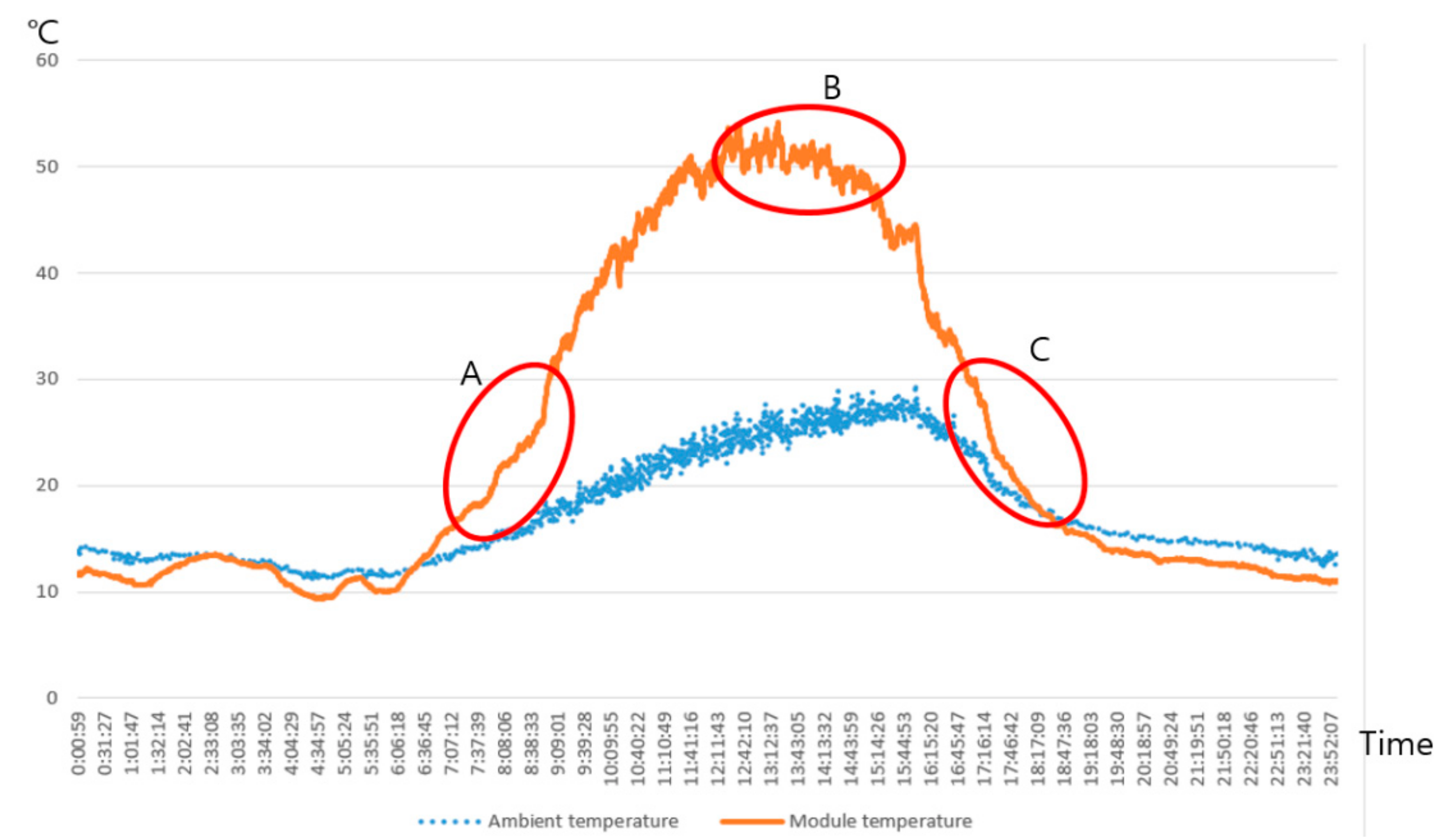The elements n and $c_0$ in Equation (15) can be characterized from the collected data. As shown in Figure 4, when the module starts to generate electricity, the PV module temperature rises to generate electricity. Assuming 1000 W/${\mathrm{m}}^2$ of solar radiation is generated, electricity is converted to 15%–20%. The remaining energy is energy related to heat, which is consumed outside the module rather than PV module inside like convective energy. However, PV module temperature rises due to the presence of remaining thermal energy generated and accumulated. There is a large difference between ambient temperature and PV module temperature. PV module temperature is inevitably higher than the ambient temperature. The higher the PV temperature, the lower the generation due to the characteristics of the PV module temperature change. In addition, the reason that voltage is affected by temperature and current is affected by insolation is also due to characteristics of the PV module temperature change.

The conversion coefficient n and $c_0$ is calculated as follows.

First, a region, such as part B in Figure 4, where the module temperature does not rise or fall, is identified with clear irradiation and low wind speed (2 m/s or below). Temperature that does not change (rise or fall) means that $\Delta \mathrm{T}$ = 0. Therefore, the following equation becomes valid:

$$0=I_{r\left(t\right)}-P_{m\left(t\right)}-c_0\left(T_{m\left(t\right)}-T_{A\left(t\right)}\right).$$

(16)

After identifying $c_0$ here, the n value can be determined by using the data in part A of Figure 4. $c_0$ can be expanded as below to include the wind effect [3,4,5].

$$c_0=c_1+c_2\times WS$$

(17)

where

• $c_1$: Fixed conversion coefficient value (W/m² °C);
• $c_2$: Conversion value of wind speed (W/m³ °C).

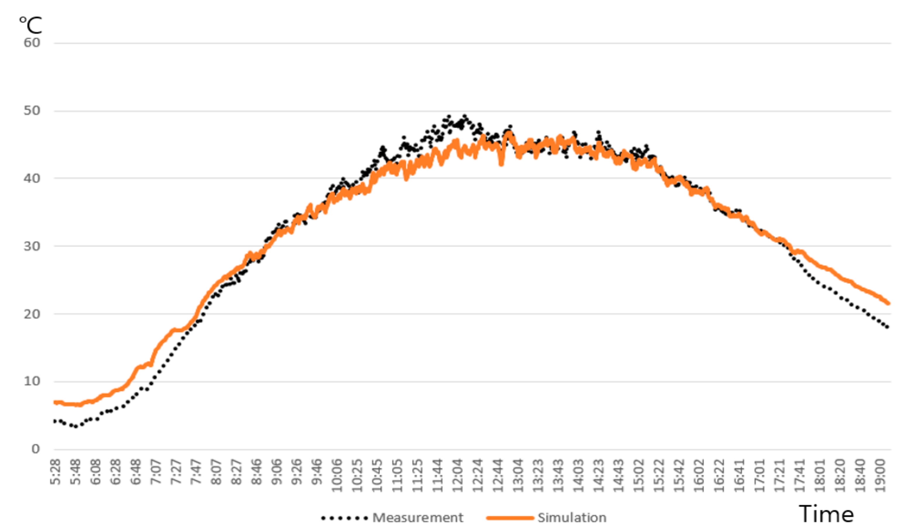
The initial $c_0$ becomes $c_1$, as it is the conversion coefficient identified when the wind speed was low. After identifying $c_1$ and n, $c_2$ can be identified, based on the data of the date with wind speed that is higher than a certain value. In addition, it is necessary to verify the value of n, $c_0$ by looking at the entire point through the graph in Figure 4. In the case of 200~900 W/${\mathrm{m}}^2$ or more based on insolation, the average values n and $c_0$ are obtained by dividing a total of 8 sections and after substituting into Equation (15) and simulating. However, due to KS C IEC/TS 61724-2:2016, the minimum POA insolation intensity during the four seasons is more than 450 W/m². Then, 6 equations with different n, $c_0$ are expressed. Among the regressing analysis methods, if the RMS (Root Mean Square) error is used and a combination of coefficients when the RMS error of the module temperature values is minimized is used, the result of conversion coefficient can be more accurately expressed [11,12].

3. Results

As a result of applying Equation (15) to the measured 265 W PV module in this study, the extracted coefficients are n = 2.33 (°C m²)/W, $c_1$ = 33.26 W/(m² °C), and $c_2$ = 5.31 W/(m³ °C)). The measured and calculated daily change in module temperature for one day is presented in Figure 5. The mean difference was 1.64 °C and the maximum difference was 5.63 °C. In addition, the difference between the actual energy generation and the predicted generation was approximately 5.2%, as shown in Figure 6.

The results that were better than the mean error of 4.23 °C, calculated with the Equation (1), are shown. Figure 7 shows the results of the module temperature predicted by using the Sandia National Laboratory equations [12,13].

Instances of substantial error are found in previous research results.

The existing mass-produced Si-type modules have similar values. Figure 8 indicates the results of a comparison between the predicted values and the measurement values of another 260 W mass-produced module.

The mean error of the measurements and predictions is approximately 7.53%. This shows that the Si-type modules have a similar trend.

4. Conclusions

With regard to the temperature rise of the PV module, the prediction of the module temperature showed slight differences in a shorter time than when thermal equilibrium occurs and as compared with the existing research results. In other words, the temperature or generation is usually predicted at intervals of more than one hour, but this experiment can be predicted in real-time in seconds or minutes. Therefore, the shorter the interval, the smaller is the error. For this, a new prediction equation was suggested and was implemented in this experiment. The results indicate that prediction was possible within an error range of approximately 5% in comparison with the actual generation. Obviously, not all the modules have the same conversion coefficient; however, the Si-type modules that use similar materials show similar results.

The daily irradiation, wind direction, and wind speed data could vary; however, the annual average does not show substantial changes. If there were an annual or longer period data of irradiation, air temperature, and wind speed, the annual generation in the actual outdoor condition could be predicted by weeklong tests or 10-day tests on the new module. In addition, the results of the current study can be comparatively analyzed with several modules. Such comparison is needed to develop modules with improved performance.

In addition, studies on the influence of humidity on the module temperature should be performed. Clearly, the temperature changes in the module would be different in dry desert regions and in humid tropical regions. The n, $c_1$, and $c_2$ values that were calculated in this study could vary depending on regions, and new variables could be added. Therefore, to promote research in this wide field, the environmental data of various climates should be accumulated and shared.

This experiment was supported by the equipment and technology of Yeungnam University Daekyung solar cell regional innovation center.

References

1. Kim, M.S. Optimal Design for Silicon Based Photovoltaic System. Master’s Thesis, Yeungnam University, Gyeongsangbuk-do, Korea, 2006. [Google Scholar]
2. U.S. Department of Energy. 2010 Solar Technologies Market Report; U.S. Department of Energy: New York, NY, USA, 2011; pp. 21–25.
3. Lking, D.; Boyson, W.E.; Kratochvil, J.A. Photovoltaic Array Performance Model; Sandia National Laboratories: Albuquerque, NM, USA, 2004; pp. 7–18. [Google Scholar]
4. Mavromatakis, F.; Kavoussanaki, E.; Vignola, F.; Franghiadakis, Y. Measuring and Estimating the Temperature of Photovoltaic Modules. Solar Energy 2014, 110, 656–666. [Google Scholar] [CrossRef]
5. David, F. Assessing the Outdoor Operating Temperature of Photovoltaic Modules. Prog. Photovolt Res. Appl. 2008, 16, 307–315. [Google Scholar]
6. Adeh, E.H.; Good, S.P.; Calaf, M.; Higgins, C.W. Higgins Solar PV Power Potential is Greatest over Croplands. Sci. Rep. 2019, 9, 1–6. [Google Scholar] [CrossRef] [PubMed]
7. Ashrafizadeh, S.A.; Tan, Z. Mass and Energy Balances Basic Priciples for Calculation, Design, and Optimization of Macro/Nano Systems; Springer: Berlin, Germany, 2018; pp. 127–130. [Google Scholar]
8. Holman, J.P.; Kwon, Y.P. Heat Transfer, 8th ed.; McGraw Hill Companies: Seoul, Korea, 1997; pp. 2–18. [Google Scholar]
9. Bird, R.B.; Stewart, W.E.; Lightfoot, E.N. Transport Phenomena; Wiley: New York, NY, USA, 1960; p. 245. [Google Scholar]
10. Smith, J.M.; Van Ness, H.C.; Abbott, M.M.; Swihart, M.T. Introduction to Chemical Engineering Thermodynamics, 8th ed.; McGraw Hill: Boston, MA, USA, 2001; pp. 52–53. [Google Scholar]
11. IEC TS 61724-2:2016. Photovoltaic System Performance—Part 2: Capacity Evaluation Method; IEC: Geneva, Switzerland, 2016; p. 27. [Google Scholar]
12. Mikofski, M.; Andeerson, M.; Caldwell, S.; DeGraaff, D.; Hasselbrink, E.; Kavulak, D.; Lacerda, R.; Okawa, D.; Shen, Y.-C.; Tediasaputre, A.; et al. A dynamic cell-by-cell PV system model to predict lifetime performance and reliability. In Proceedings of the 26th European Photovoltaic Solar Energy Conference and Exhibition, Hamburg, Germany, 5–9 September 2011; pp. 105–112. [Google Scholar]
13. King, D.L. Photovoltaic Module and Array Performance Characterization Methods for All System Operating Conditions. AIP Conf. Proc. 1997, 394, 347–368. [Google Scholar]
Figure 1. Prediction of module temperature using existing temperature prediction equation.
Energies 14 01503 g001
Figure 2. Fixed testbed system with the maximum setup of eight modules. The data time step is 30 s.
Energies 14 01503 g002
Figure 3. Global Normal Irradiance (GNI), ambient temperature (1–17 May 2015).
Energies 14 01503 g003
Figure 4. Graph of ambient and module temperatures (10 May 2015).
Energies 14 01503 g004
Figure 5. Photovoltaic (PV) module temperature graph showing measurement and prediction (05 May 2015).
Energies 14 01503 g005
Figure 6. PV module power generation graph showing measurement and prediction (05 May 2015).
Energies 14 01503 g006
Figure 7. Graph showing the results of the current study and that of other studies.
Energies 14 01503 g007
Figure 8. Graph of the measurement values and predicted values of the other module (02 March 2016).
Energies 14 01503 g008
Publisher’s Note: MDPI stays neutral with regard to jurisdictional claims in published maps and institutional affiliations.