1. Introduction
Due to the large use of transformers, their accurate rating is crucial to avoid faults and guarantee secure and reliable operation of power systems. The task of transformer rating is typically performed through the estimation of the lifetime duration under a predicted loading condition. Lifetime duration strictly depends on the degradation of solid insulation, which is the primary reason why a transformer reaches the end of its life. Continuous degradation mainly occurs because of thermal stresses which affect transformers as a consequence of the heat generated during operation [
1]. Thermal models are available in the literature and are used in consolidated international standards, such as the IEC Std 60076 [
2]. Based on the loading current, they provide accurate estimations of the temperatures affecting the heat-sensitive parts of the transformers which are used in lifetime calculation.
Methods for transformer rating consist of choosing the size of the transformer which better fit the expected current flowing in the transformer with the desired lifetime duration, thereby avoiding accelerated degradation. The key aspect to optimize the determination of the transformer size relies in the determination of loading condition, which is a very complex task in modern power systems being subject to large uncertainties and random time disturbances, which affect all aspects of the operation of the system. Fluctuation in the power demand and intermittent nature of renewable generation are the most significant examples. It is also well known how challenging is to plan both the electric grid and the various components due to continuous power variations. In the case of transformers, aspects of uncertainties need to be carefully considered in order to accurately determine loading conditions [
3].
This paper focuses on an accurate method for the optimal rating of oil-immersed power transformers connected to wind farms. The effect of fast variations of wind velocity implies that the transformer can be repeatedly overloaded without impacting on the loading current mean value but causing overheating, thus implying an erroneous sizing of the transformer. With conventional approaches, transformers connected to power plants are sized by assuming that all of the generators output their rated power without considering fluctuations which inherently characterize renewable power generation. It is then required to include this effect to have a more accurate sizing [
4].
In the technical literature, rating of power transformers that connect wind power plants to the grid is investigated in [
5], where a dynamic approach for exploiting the variability of power production is proposed. In [
6] a cost optimization methodology is proposed which uses statistical scenarios based on distribution functions and Markov Chain models and accounts for maintenance and design requirements for transformer contingency in off-shore wind farms. The calculation of transformer limits according to the shape of the loading profile in presence of renewable generation is analyzed in [
7], where an energy-limit concept for oil-immersed technology is proposed. Based on the loading factor, in [
8] a method to size the power transformer using the thermal limit is proposed. The potential of dynamic rating in the planning stage of transformers for renewable sources is analyzed in [
9] to utilize equipment more efficiently. In [
10] a stochastic method is used to characterize daily loading profiles in the presence of fluctuations to evaluate their impact on the transformer lifetime. In [
11] a rating method is proposed based on measured and estimated daily loading profiles. In [
12] a data driven approach based on a Gaussian mixture mode is used to estimate the loading shape profile for the transformer rating at the purpose of long-term planning. Randomness of loading profiles in the presence of fluctuations are addressed in [
13] through a Lognormal characterization of transformer lifetime for its power rating. The maximum utilization transformers through dynamic thermal rating is studied in [
14] with reference to loading with random variations.
The analysis of the literature survey provides evidence of some critical issues that need to be addressed in the transformers’ rating, such as: (i) analysis of the loading conditions, (ii) thermal behavior of the transformer under specified loading conditions, (iii) estimation of the expected lifetime duration under specified loading conditions, and (iv) evaluation of the transformer size that better matches the desired lifetime and expected loading duration.
The analysis of the loading condition is clearly the main input of the design stage, where randomness, such as that regarding the fluctuation typical of wind farm applications, is faced with stochastic approaches, such as Markov Chain models [
6], the Gaussian mixture [
12], or the Wiener process [
13]. In this regard, the proposed approach suggests and validates a novel rating method based on the statistical characterization of the loading condition through the Ornstein-Uhlenbeck process. This stochastic process appears particularly suitable for the description of the phenomenon under investigation for its ability in capturing the so-called ‘mean reversion’ of time series [
15]. Based on the Ornstein-Uhlenbeck characterization of the loading current, the thermal description of the transformer is stochastically characterized as well. The solution of the thermal model, which is given by means of the Euler-Maruyama model, allows estimating lifetime reduction according to a Lognormal distribution. This is useful to derive an analytical method for the transformer sizing. Acceleration of lifetime reduction is avoided by selecting a transformer size larger than that obtained through the classical approaches based on average values of the loading current.
The paper is structured as follows:
Section 2 describes the process used to stochastically characterize the wind power generation.
Section 3 gives the details of the thermal model used for estimating the lifetime of a mineral-oil-immersed transformer and lifetime characterization in terms of stochastic processes. In
Section 4 the analytical formulation of the transformer rating is calculated and the whole procedure is summarized. In
Section 5 the results of the proposed rating method applied to the data of a wind farm are reported. Conclusions are drawn in
Section 6.
2. Stochastic Characterization of the Wind Power
Many studies are available in the literature to properly characterize wind power randomness [
16,
17]. Among them, two approaches are typically used: static [
18,
19] and dynamic approaches [
20,
21]. The dynamic approach based on the stochastic process theory is the most suitable in order to achieve a more accurate characterization of the wind power behavior. As proposed in [
20], the Ornstein-Uhlenbeck stochastic process appears particularly adequate to describe the random variations of this non-controllable energy source.
Indeed, the Ornstein-Uhlenbeck stochastic process is largely employed as a diffusion process to model several phenomena, as in the processing of financial high-frequency data. With respect to the power system, it is considered particularly suitable to describe the electrical load [
22]. The rationale behind this choice relies in capturing the so-called ‘mean reversion’ of certain time series, which tend towards their mean values over the time. The Ornstein-Uhlenbeck process
,
, is wholly described by the following stochastic differential equation:
where
µ is the long-term mean,
τ is related to reversion speed, σ is linked to the instantaneous volatility, and
is the Wiener process characterized by the well-known property that
has independent increments with
(for
), with
as the normal distribution with expected value 0 and variance
t −
s.
It is important to note that, if , then and are independent random variables. Also, the following probabilistic properties can be derived:
- -
the unconditional probability density function at a fixed time t is Gaussian:
- -
the expectation is zero:
- -
the variance at time t is:
- -
the covariance at time t is:
The solution of the stochastic differential equation is given by:
The Ornstein-Uhlenbeck process
is stationary when
and
are assumed and has normally distributed increments and unconditional moments:
Non stationarity of the problem was attained for a given initial value
with normally distributed increments and conditional moments:
In order to investigate the problem of the process parameter estimation, the discrete version of the process is referred to here where, for the sake of simplicity, the time interval is assumed to be equal to 1. The process has observations at time instants , where .
By referring to the discretized version of the process, the method of moments was applied for its simplicity. It is not difficult to demonstrate that the following relationships maintain as far as the estimate is concerned for the parameters
μ,
τ and
σ2 [
22]:
In practice, the actual observed process could be corrupted by a noise
Ei; as a consequence of that, the following process should be examined:
Under the assumption
E~
N(0,
ν2), we could obtain:
In this case, the estimates for
µ,
τ,
and ν
2 can be given by the following relationships:
3. Stochastic Thermal Model of a Mineral-Oil-Immersed Transformer
With lifetime evaluation being the core of the transformer’s design, the dynamic aspect of the thermal phenomena and their stochasticity due to the loading needed to be properly taken into account.
The thermal processes of mineral-oil-immersed transformers were modeled based on the top-oil and hot-spot temperatures. Top-oil temperature refers to the oil temperature at the top of the tank; hot-spot temperature refers to the temperature of the hottest point of the winding insulation. The measure of the top-oil temperature is simple and thus is suitable for on-line monitoring and control of the transformer. Hot-spot temperature is related to the loading capacity of the transformers and their lifetime degradation [
23,
24].
Regarding the top-oil temperature, the values it assumes depend on the heat generated by the Joule losses in the windings (i.e., load losses) and no-load losses, the ambient temperature, and the thermal characteristics of the oil. Regarding the hot-spot temperature, the values it assumes depends on the heat generated by the load losses, the temperature of the oil, and the thermal characteristics of both winding and oil [
25,
26,
27,
28,
29]. In the case of a significant presence of non-linear loads or converter-based generators, the loads due to non-sinusoidal voltages can have a role in the thermal behavior of the transformer and consequently on its lifetime [
30,
31,
32].
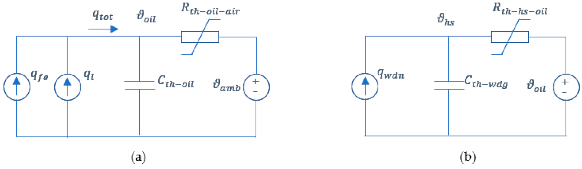
Estimation of both top-oil and hot-spot temperatures is typically made by thermal models which exploit the thermal-electrical analogy and heat transfer theory [
1]. The thermal-electrical analogy theory is based on the use of simple circuits which allow analyzing the thermal behavior of the transformers through the similarity between thermal and electrical processes. Based on this approach, top-oil (
) and hot-spot (
) temperatures vary according to differential equations of resistive-capacitive lumped circuits forced by ideal sources related to heat generated in the transformer [
1,
33,
34]. In
Figure 1, the circuits related to the top-oil temperature (
Figure 1a) and hot-spot temperature (
Figure 1b) are reported.
In
Figure 1a the total heat generated in the transformer (
) refers to the heat generated by no-load losses (
) and by the load losses (
),
is the equivalent thermal capacitance of the transformer oil,
is a nonlinear oil to air thermal resistance, and
is the known ambient temperature. In
Figure 1b
is the heat generated by winding losses,
is the thermal capacitance of the winding, and
is the nonlinear winding to oil thermal resistance. Non-linear thermal resistances in the circuits are considered to include the effect of the temperature on both oil thermal characteristics and Joule losses [
24,
33,
34]. The non-linear thermal resistances allow obtaining more accurate temperature estimation due to the deep dependency of the oil characteristics—particularly the viscosity—on the temperature.
The differential equations governing the thermal circuits of
Figure 1 are:
with (18) being related to the top-oil model and (19) to the hot-spot model which depends on the top-oil temperature, with the following symbols meaning:
- -
is the ratio of load losses at the rated current and no-load losses;
- -
is the ratio of load current and the rated current, i.e., the load factor;
- -
is the oil viscosity in per unit value;
- -
is the ambient temperature;
- -
is the hot-spot temperature;
- -
is the top-oil temperature;
- -
is the rated top-oil temperature rise over the ambient temperature;
- -
is the rated hot-spot temperature rise over the top-oil temperature;
- -
is the rated top-oil time constant;
- -
is the rated winding time constant;
- -
is the value of the load losses, in per unit, and
represents the dependence of these losses from the hot-spot temperature;
- -
ν and ν′ are constant and depend on the type of transformer and the cooling modes; the exponentials of ν and ν determine the non-linearity of the model.
The solution of (18) and (19) can be evaluated through classical numerical methods, such as the Runge Kutta method, if a deterministic framework is considered. As will explained in the next section, the time variations of the top-oil and hot-spot temperatures have to be derived by properly treating the stochastic variations of the known load. For this purpose, the Euler-Maruyama method was employed.
The hot-spot temperature is the main factor responsible for accelerating the transformer aging, thus its estimation is used to evaluate the lifetime reduction of the winding insulation. Ambient temperature and moisture also have influence, the latter having a significant effect since the water generated by the process of cellulose decomposition significantly accelerates its aging rate [
35,
36,
37].
The insulation deterioration in the time period
can be evaluated on the basis of experimental evidence according to [
38]:
with
being the loss of life of the transformer over the considered time period
and
being the aging acceleration factor. Regarding the duration of the time period to be considered for designing purposes, it can be assumed that
, since the working cycle is typically repeated according to daily working cycles [
39]. Regarding the aging acceleration factor
, it is governed by the well-known Arrhenius reaction rate theory, which is given by:
where the hot-spot temperature
is assumed time-varying and 110 °C is assumed as the reference temperature, i.e., the acceleration factor of degradation is evaluated based on the deviation of
from 110 °C. In this way, the lifetime decrease
was estimated through (20) in per unit measurements.
3.1. Integration of the Stochastic Differential Model
By neglecting the voltage drop across the leakage reactance, the load factor
in (18) and (19) can be considered equal to
, with
being the base power. Due to its dependence on the process
,
is properly described as random process
, as well as the ratio of load losses
, which is also described as random process
. For characterizing the stochasticity of the variables
and
, the following model had to be integrated:
The integration of this model was numerically performed by using the Euler-Maruyama method, which is opportune to briefly recall [
40]. Let us consider a scalar, autonomous stochastic differential equation written in the standard form:
The discretized version of (25) is
where
.
In (26) the only complication lies in the generation of the increments . By keeping in mind the properties of the standard Wiener process, also named standard Brownian motion, it is intuitive to assume is an independent random variable distributed according to the law . The Euler-Maruyama method is substantially summarized by Formula (26), where only the additional burden to generate random vector from the distribution is required.
It is good to make some considerations regarding convergence of this method, that is, to ascertain whether the solution tends more and more to true when
tends to zero. By denoting with
the true solution at the
ith-step, which is a random variable as
, the concept of strong convergence has to be introduced. A method exhibits strong order of convergence equal to
α if a constant
λ exists such that:
It can be demonstrated that if the functions
and
satisfy some conditions, the Euler-Maruyama method has strong order of convergence
. The concept of strong convergence is stated in terms of expected value, but useful inequality can also be derived to characterize the error for individual simulations by exploiting the Markov inequality. As is well known, this cornerstone inequality in the theory of probability states that if a random variable
has finite expected value,
:
By applying this inequality to (27), and choosing
, with
, since for Euler-Maruyam method
, it can be written as:
It can be more useful to write the relationship as:
which ensures that for any point over the interval
, the error will be small with the probability tending to
.
3.2. Lifetime Characterization
The oil transformer temperature as well as the hot-spot temperature have the character of stationary random variables. As will be numerically demonstrated in the numerical application, the mean value and the standard deviations can be considered as constant over the whole interval . More specifically the hot spot temperature can be optimally approximated by a stationary Gaussian process.
The integrand factor in Equation (20) can be rewritten as:
with
is a Lognormal process and its parameters can be expressed explicitly as a function of the moments of the stochastic process,
. The Lognormal statistical feature of
and its stationarity were verified in the numerical application reported in
Section 5 by examining the behavior of both the mean value and the standard deviation over the time.
From the earlier definition of the reduction of the transformer’s lifetime, the following relationship can be stated:
As a consequence of the stationarity of the
process, the reduction in the transformer’s lifetime
can be optimally approximated by a Lognormal random variable whose mean value is equal to
When (that is ) there is no ageing acceleration with respect to that arising with the rated values of current, . The fluctuation of the loading current around its mean value (that is the value typically used to size transformers ), however, implies an ageing acceleration (i.e., lifetime reduction) higher than that occurring for and whose value is related to corresponding to the variation of temperature due to the current’s fluctuation.
4. The Proposed Transformers Rating Procedure
The value of
(i.e., of transformer’s size) can be identified by assuming that
produces a constant temperature equal to
and the fluctuating current the contribution
By keeping this in mind, the transformer rated current can be estimated as follows:
with
From (37), it is possible to straightforwardly obtain the rated value of the current . Indeed, the design procedure has to start by initially choosing a transformer whose rated power is as near as possible to the mean value of the loading power. By making reference to its characteristic parameters, one can perform an a priori estimation of the temperature distribution. This allows directly determining that the oversizing factor for ensuring the mean value of lifetime is equal to that expected.
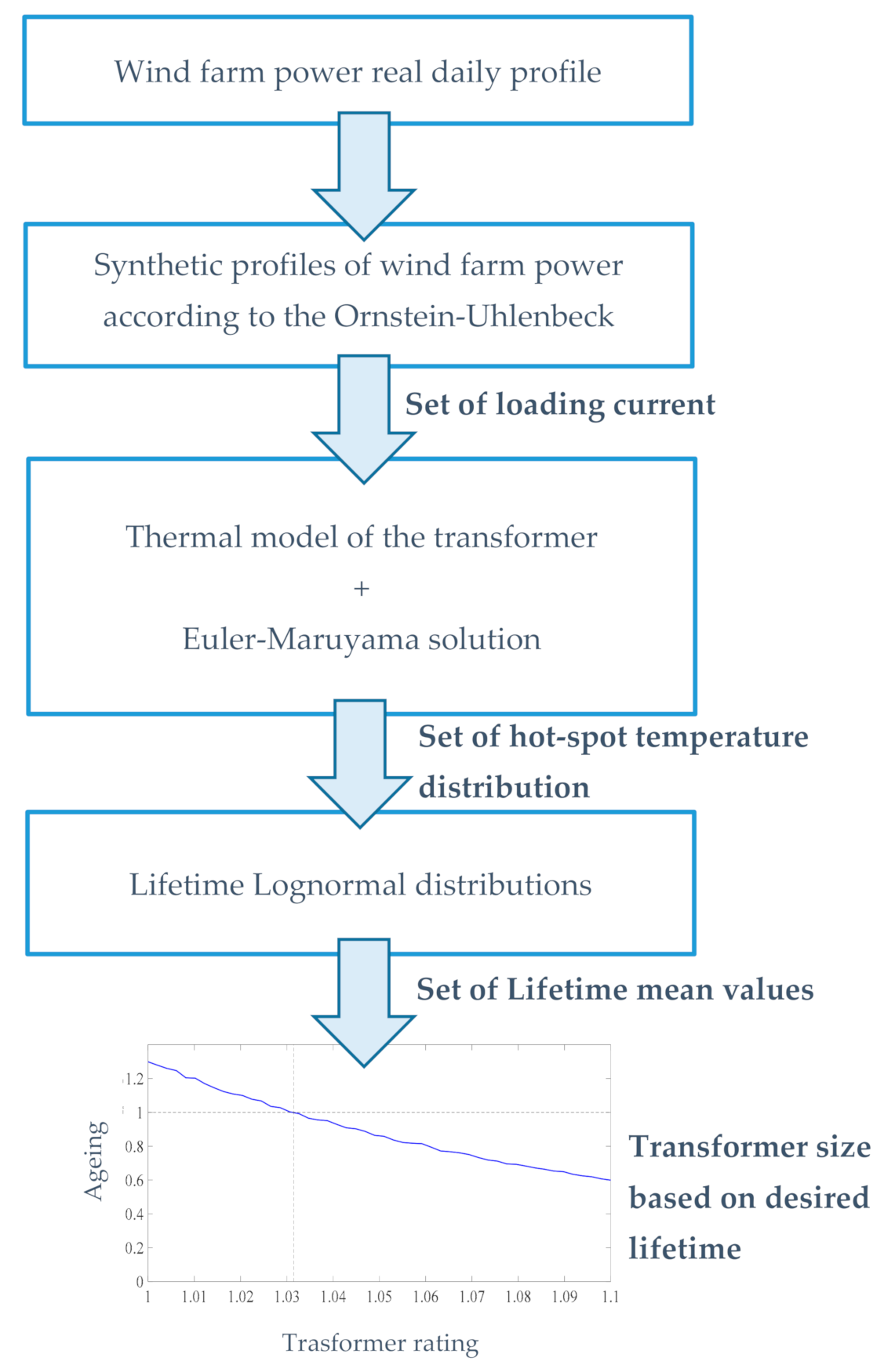
The procedure for choosing the rated power of the transformer can be eventually summarized by the flow chart reported in
Figure 2.
The proposed procedure—shown in
Figure 2—can be summarized as follows:
the actual power profile of the wind farm is recorded based on data available from measurements;
the actual power profile is statistically analysed as an Ornstein-Uhlenbeck process and a number of synthetic profiles are generated;
based on the loading current corresponding to the synthetic power profiles, the thermal model of the transformer is applied and solved in statistical terms through the Euler-Maruyama method, thus obtaining the statistical characterization of the hot-spot temperature;
on the basis of the distribution of the hot-spot temperature, the statistical characterization of the transformer’s lifetime is derived;
the rating of the transformer able to guarantee the desired lifetime is calculated through Equation (37).
5. Numerical Application
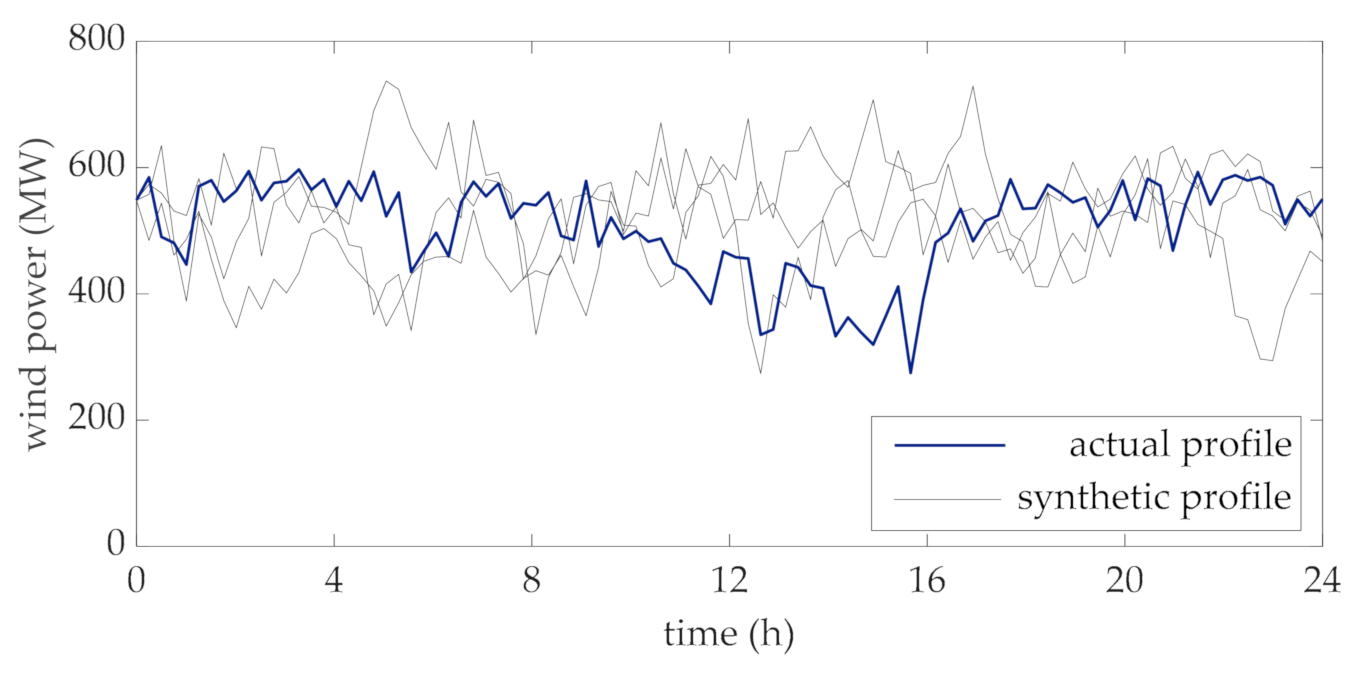
In this section, the results of the application of the proposed rating method to the data of a 600 MW wind farm are reported [
41]. Based on the measured data (step 1 of the flow chart in
Figure 2), the actual power produced by the wind farm is plotted in
Figure 3 (blue thicker line). This dataset refers to the time horizon of one day which is divided into 96 time-intervals, each 15 min long.
This daily profile is characterized as an Ornstein-Uhlenbeck process (step 2 of the of the flow chart in
Figure 2), whose parameters, estimated by the method of moments, are
,
, and
. Some realizations of the process (i.e., synthetic profiles), by employing these parameters, are also reported in
Figure 3 (gray lines).
The rating of the transformer connecting the wind farm to the network was performed according to the method proposed in this paper. The parameters used in the thermal model were derived from a typical 605 MVA OFAF transformer [
33] and are reported in
Table 1. The ambient temperature was assumed to be constant (30 °C), since the assumption was made that a confined ambient environment equipped with a cooling system would almost guarantee a constant temperature. Regarding the oil thermal conductivity, its variation with the temperature was negligible compared to the variations of the oil viscosity [
32]. Thus, the approximation of constant thermal conductivity corresponding to 65 °C was assumed. Both
C and
ν are empirical constants whose values correspond to the case of laminar oil circulation [
32].
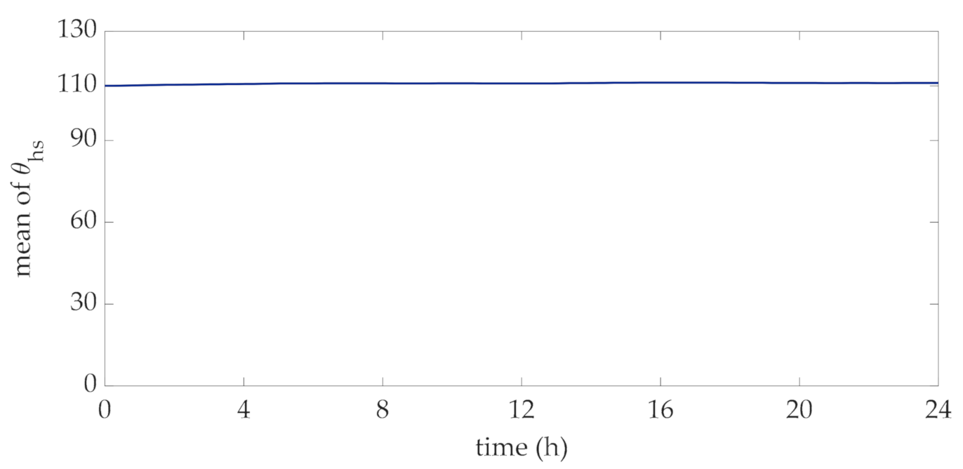
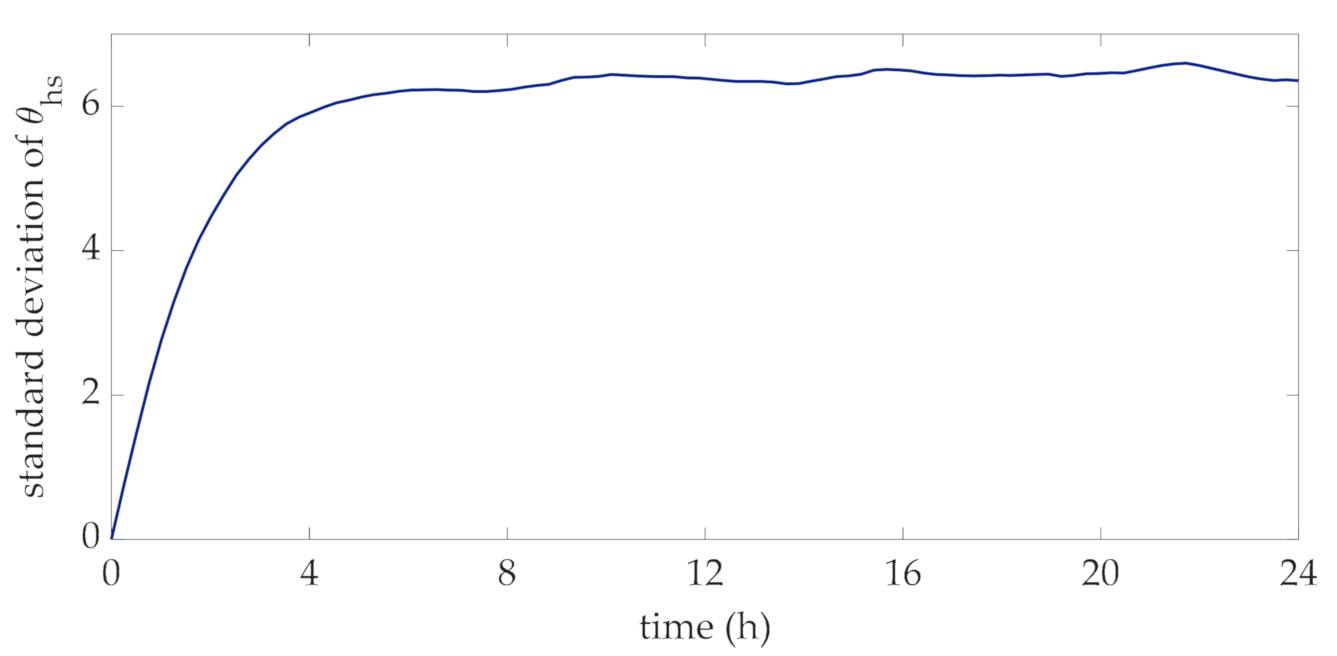
In order to perform the proposed method for the choice of the transformer rating, 10,000 daily profiles of wind power were obtained through the statistical characterization of the Ornstein-Uhlenbeck approach. These profiles were used to derive the distribution of hot-spot temperature at each time interval of the day. With reference to the rated currents corresponding to the mean values of this data set, in
Figure 4 and
Figure 5 the mean value and standard deviation of this temperature at each interval are reported. The mean values reported in
Figure 4 reveal that they vary within a narrow interval around the rated hot-spot temperature, i.e., 110 °C, which corresponds to a standard lifetime duration assumed for the transformer. The profile of the standard deviation at each interval reported in
Figure 5 clearly converges to a specific value, thus showing that the considered process can be assumed to be stationary.
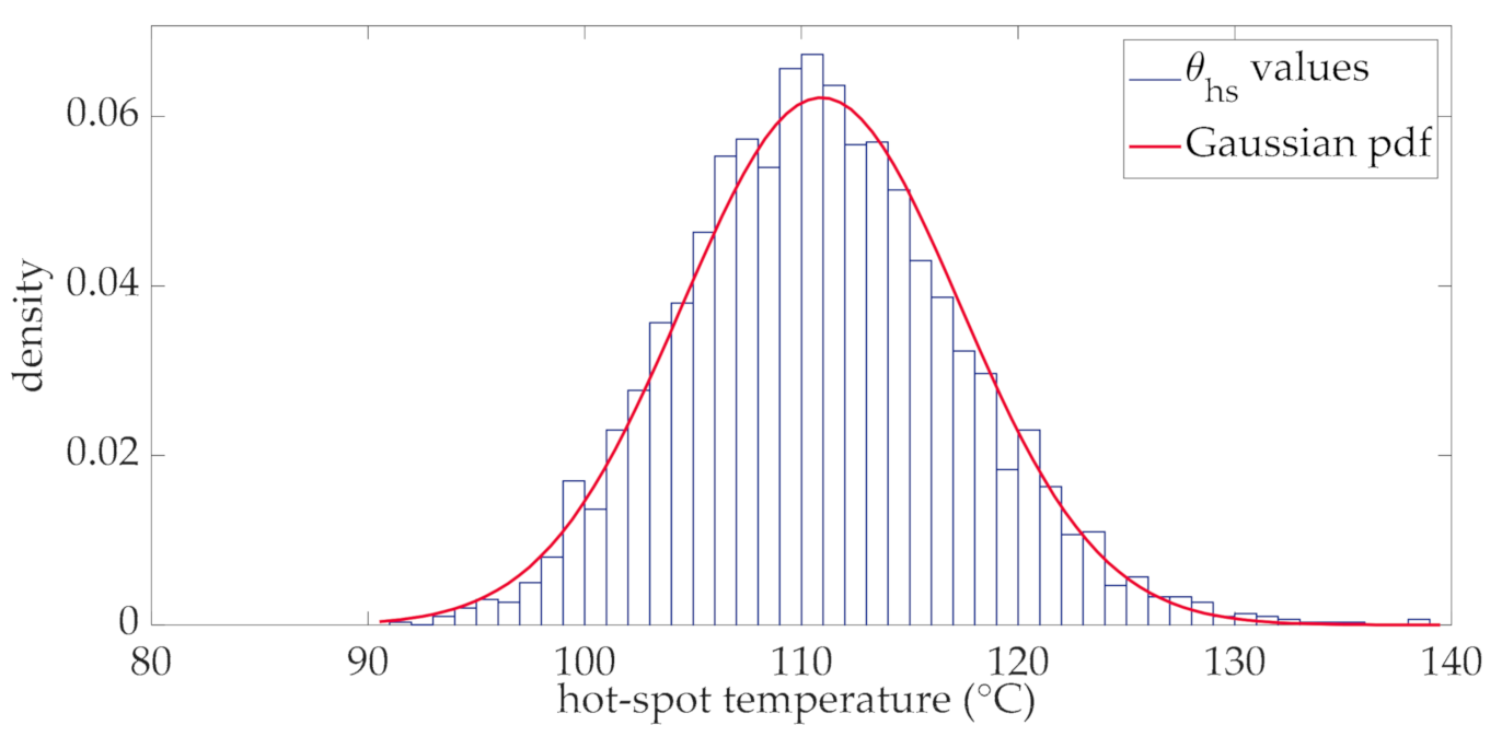
Regarding the hot-spot temperature, it can be stated that its distribution at each interval is Gaussian. This is verified by the results obtained by the adoption of the thermal model of
Section 3 (step 3 of the of the flow chart in
Figure 2). Particularly in
Figure 6, the histogram of the hot-spot temperature corresponding to a generic interval of the day (the interval corresponding to the 12th hour) is reported together with its fitting Gaussian probability density function (pdf) which shows a good approximation with the simulated data. Mean value and standard deviation of this distribution are
°C and
°C.
The accurate Gaussian approximation shown in
Figure 6 is coherent with the assumption of the Ornstein-Uhlenbeck model. The analysis of the other intervals of the day, not reported here for the sake of brevity, shows that this Gaussian approximation is also valid.
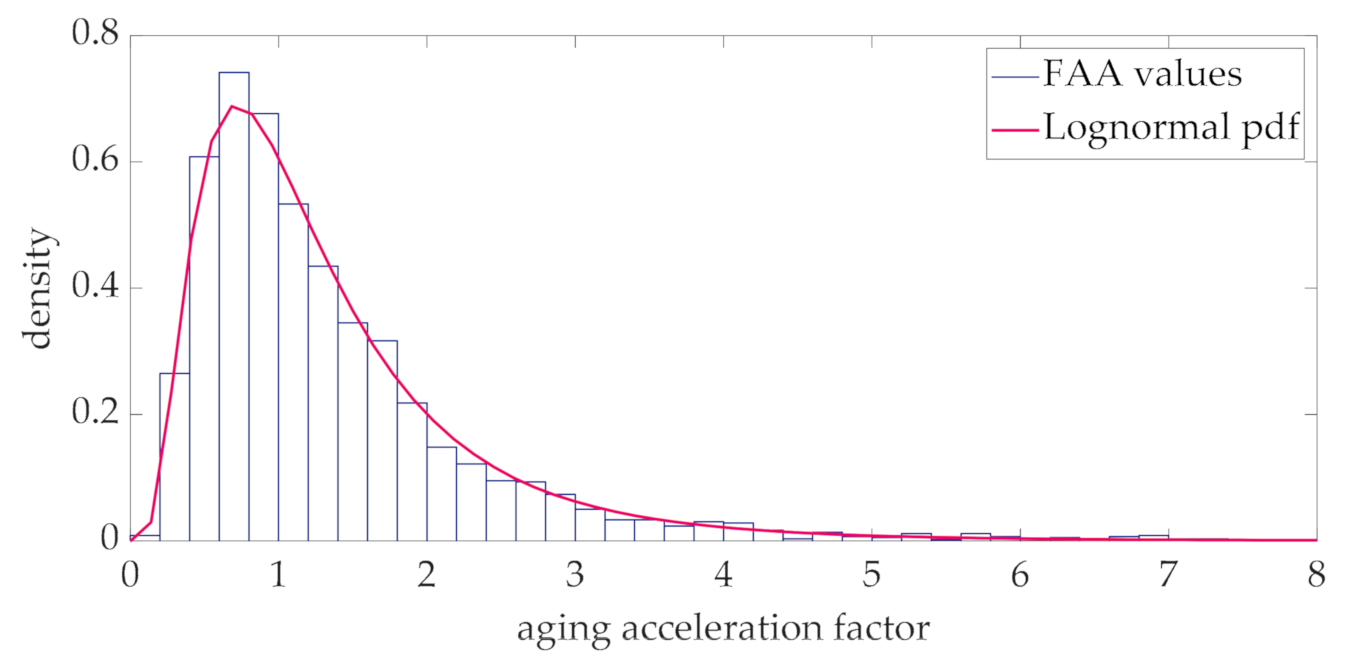
The distribution of the aging acceleration factor at the same interval of
Figure 6 is reported in
Figure 7.
As expected, this distribution is well fitted by a Lognormal distribution, whose pdf is also reported in the figure. The analysis of the other intervals of the day, here not reported for the sake of conciseness, shows that this Lognormal approximation is also valid. This approximation is coherent with (31) and with the Gaussian approximation of the hot-spot temperature at each interval of the day (
Figure 6).
As is well known, the Lognormal distribution can be represented in its general form as:
where
and
are the mean and standard deviation of the associated Gaussian distribution (
and
in our case).
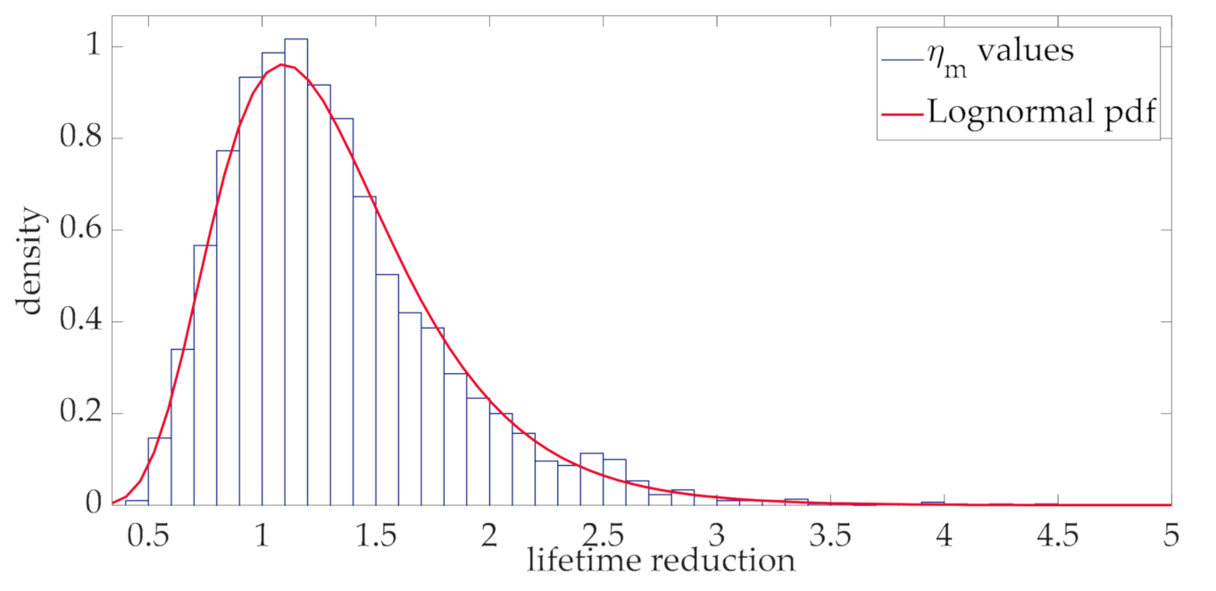
Based on the Lognormal process of the aging acceleration factor, the distribution of lifetime reduction in per unit values was derived and is shown in
Figure 8 (step 4 of the of the flow chart in
Figure 2).
Coherently with the theoretical hypothesis made in
Section 3, it was found that the distribution of the lifetime reduction values is well approximated by a Lognormal pdf, as clearly appears in
Figure 8. This can be explained by considering that the lifetime is evaluated by means of (34) and the aging acceleration factor (31) is well approximated by a Lognormal distribution at each interval (
Figure 7). In this case, even if the sum of Lognormal distributions is not generally lognormally distributed, the stationary property of the process implies that the Lognormal distribution can still be used to represent the integral in (34). It is worth noting that this result has general validity, since it derives from the statistical characterization of the wind power according to the Ornstein-Uhlenbeck stochastic process and a consolidated thermal model of transformers. In order to apply the proposed procedure at the design stage of the transformer with the purpose of choosing the rating of the transformer, the proposed approach was repeatedly applied by increasing values of the rated transformer current, as recalled in the flow chart of
Figure 2 (step 5 of the flow chart in
Figure 2).
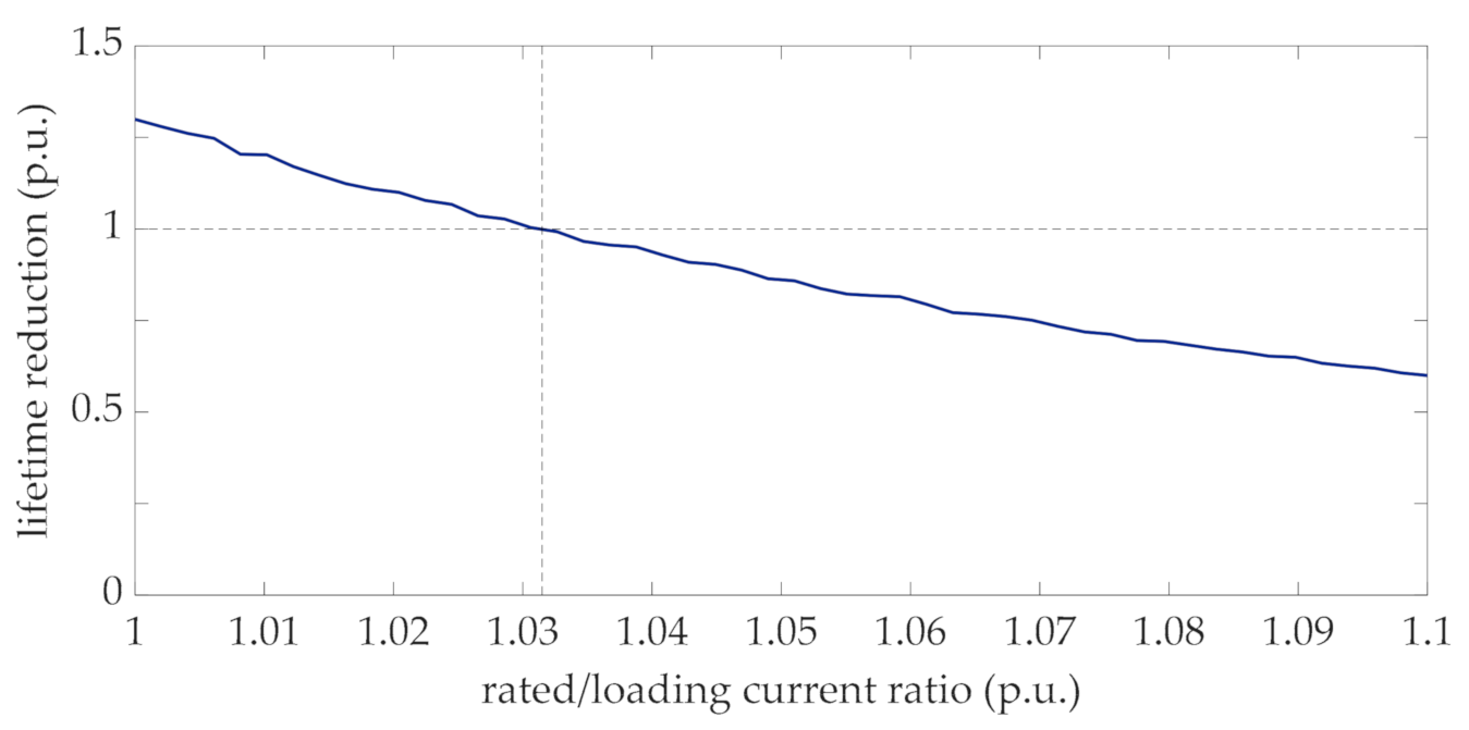
Figure 9 shows the lifetime reduction corresponding to the ratio
of the rated and mean values of the loading current.
Figure 9 clearly shows that the reduction of lifetime—compared to the duration corresponding to the standard hot-spot temperature (110 °C) decreases when the rated current increases. Particularly, with reference to the proposed case study, the lifetime reduction is equal to one when the rated current is 1.032 times greater than the mean value of the loading current. For lower values of the rating current the reduction of lifetime is greater than one, reaching a value higher than 1.25 in case of rated current equal to the mean value of the loading current. This means that by applying conventional rating methods, i.e., by neglecting the effect of fluctuations of the generated power, the expected lifetime of transformer would be reduced by 25%. Alternatively, to avoid this reduction, a de-rating of the transformer would be needed.
Figure 9 also shows that in the case of higher values of rated current (i.e., abscissa greater than 1.032) a slow reduction of lifetime appears (i.e., its values are lower than one), reaching the value of 0.6 when the rated/loading current ratio is 1.1.
In order to analytically derive the increased rated current identified in
Figure 9, Equation (36) was also applied with
and
. Coherently with the result of
Figure 9, the rated current corresponding to the rated hot-spot temperature was equal to 1.032. This result once again shows the validity of the hypothesis that lifetime reduction is lognormally distributed, as derived in
Figure 8.


