Enhanced Model Reference Adaptive Control Scheme for Tracking Control of Magnetic Levitation System

Abstract

Magnetic Levitation is a process in which an object is suspended with the support of the magnetic field. Despite being an unstable system, Magnetic Levitation Systems (MAGLEV) have profound applications in various fields of engineering. MAGLEV systems are sensitive, unstable, and nonlinear and uncertainties always pose a challenge in Controller Design. As a solution, adaptive controllers came into existence with adaptation mechanisms to cover the system uncertainties. In this study, a simple, novel, and an effective approach to the Enhanced Adaptive Control scheme is proposed for the ball position control and tracking of an unstable Magnetic Levitation System. The proposed Enhanced Model Reference Adaptive Scheme (EMRAC) follows the same phenomenon of the Model Reference Adaptive Scheme (MRAC) with a slight difference in its control strategy. The proposed scheme consists of Proportional-Integral-Velocity plus Feed Forward as the control structure and a modified version of the standard tuning rule is used as the adaptation mechanism. The control scheme is applied to a standard benchmark Magnetic Levitation System and the tracking performance of the scheme is tested by applying square and multi-sine pattern trajectories to the Magnetic Levitation System. The performance of the developed Enhanced MRAC performance is compared with that of the Proportional Integral Velocity with Feedforward Control (PIV+FF) scheme and the proposed control scheme is proven to be more suitable. The performance of the proposed scheme is also analyzed with Power Spectral Density and Root Mean Square Error to evaluate the ball position tracking control. It is inferred from the experimental results that Enhanced MRAC accommodates the changes and makes the system more reliable with good tracking ability.

1. Introduction

A Magnetic Levitation System (MAGLEV) involves the suspension of an object by utilizing a magnetic field and by counteracting the effects of the gravitational force. It is an unstable nonlinear system so the conventional linear feedback controllers, such as P, PI, and PID controller schemes, may not be holding good performance due to the variations in the process dynamics, external disturbances, and model uncertainties associated with the non-linear unstable processes. To cope up with such non-linearities and model uncertainties, after various research studies in the field of Control Theory, Adaptive Control Schemes came into existence in the 1960s. MAGLEV has gained remarkable attention in recent years due to its applications in various fields, such as transportation engineering, environmental engineering, aerospace engineering, military weapons engineering, nuclear engineering, automotive engineering, and biomedical engineering [1]. They find their emerging utilization in magnetically levitated trains, flying cars, aircraft, wind turbines, and even in the biomedical field. This system is sensitive to environmental disturbances, such as light intensity, wind, and opposition to gravitational force. To overcome such uncertainties and effectively control the ball position and tracking, a modified version of the Model Reference Adaptive Controller (MRAC) called Enhanced Model Reference Adaptive Controller (EMRAC) is proposed, which results in a very minimal tracking error and improved performance. Initially, a Proportional Integral Velocity (PIV) controller is developed as per system requirements. Then, a novel combination of PIV with MRAC is carried out. The objective behind the study is to propose an adaptive control scheme named Enhanced Model Reference Adaptive Controller (EMRAC), which is slightly different from the standard Model Reference Adaptive Control Scheme (MRAC) to levitate a steel ball to the required position against the gravity using electromagnetic force and validate the ball position tracking control. Initially, the control schemes are simulated in MATLAB. Subsequently, the proposed control schemes are implemented and validated over a standard real-time Benchmark MAGLEV manufactured by Quanser Educational Solutions with its own Quanser real-time control (QUARC) software and are interfaceable with the MATLAB environment. The following subsections present a theoretical insight on the MAGLEV system, which is the mathematical modelling of the system followed by the controller synthesis for the proposed control scheme. The controller’s performance efficacy is analyzed with different input trajectories and a comparative analysis between the proposed control scheme and the conventional control scheme.

1.1. Theoretical Introduction

The MAGLEV system consists of three parts: solenoid coil, steel ball, and photosensor, as shown in Figure 1. The same benchmark system is used in this study. The solenoid coil provides the essential electromagnetic force for the ball to levitate. The steel ball is the object used for levitation and the post where the steel ball rests also consists of a photosensor to sense the ball position. In addition to that, the system is also provided with interior lights for visibility [2].

Adaptive controllers have gained wider attention because of their ability to adjust automatically to the unknown disturbances and model uncertainties occurring in the system. Among the adaptive control schemes, the Model Reference Adaptive Control (MRAC) finds its wider application in non-linear systems because of its simplicity and its ability to fine-tune the response characteristics of any system using a reference model [3]. The MRAC structure consists of four major components: the process model, the reference model, the control scheme, and the adaptation mechanism. Research studies are carried out with variations in a control scheme, such as Proportional Integral and Derivative (PID) with intelligent controls or optimal control schemes, and variation in the adaptation mechanism with more heuristic approaches for several kinds of applications [4]. Various controllers were implemented for the MAGLEV system in the literature, which is discussed as follows. A Static and Dynamic Sliding Mode Control (SMC) was implemented for MAGLEV to enhance the robustness for the variation in the system parameters [5,6]. Adaptive learning rules are used to learn the unknown parameters [7]. An adaptive robust nonlinear controller was proposed for the position tracking problem of a magnetic levitation system. However, the sensor measurements were found to be inaccurate due to continuous occurrences of disturbance. A combination of adaptive and robust control was found to improve the transient behaviour of the system and the same was verified by simulation and Finite Element Analysis (FEA) [8]. A non-linear Model Predictive Control (MPC) was proposed by deriving a non-linear dynamical model of the MAGLEV system and it achieved high performance for the stabilization and rapid set point changes of the levitating object. A robust controller was designed by combining the feedback linearization and H-infinity controller to control the ball position and mitigate the effects of external disturbances [9]. Feedback linearization controllers were also implemented to attenuate high-frequency disturbances. The progress in superconducting MAGLEV technology is encouraging innovations in MAGLEV transportation applications. Automatic controllers are designed for non-linear MAGLEV systems in which the controller parameters were tuned automatically using metaheuristic algorithms, which enhances design flexibilities [10]. A comparative analysis of MIT tuning rule-based control and Differential Evolution (DE) algorithm-based control was carried out for a MAGLEV system. The analysis revealed that the DE-based offline tuned PID controller performance is better than that of the MIT rule-based online tuned PID controller [11]. While in the usage of adaptive control schemes, in a standard MRAC, to rapidly reduce the tracking error, high-gain control behaviour is exhibited by using larger adaptive gain to achieve fast adaptation. Such a high gain control produces high-frequency oscillations leading the system to instability. Therefore, a faster adaptation approach was proposed based on minimizing the squares of the tracking error without affecting the robustness [12]. Also, various MRAC schemes were proposed based on different controller approaches and adaptation mechanisms [13,14,15]. In this study, a simple control approach with adaptation capability is applied to the MAGLEV system. The performance of the proposed Enhanced MRAC scheme is compared with that of the conventional Proportional Integral Velocity with Feedforward Control (PIV+FF) scheme. One of the simplest and the most effective adaptive control scheme is the Model Reference Adaptive Control Structure (MRAC), as shown in Figure 2. As the name suggests, the scheme is employed with a reference model $\left(R_M\right)$. The deviation $\left(e\right)$ between the output of the actual plant model $(y_p)$ and the reference model $\left(y_m\right)$ is periodically corrected using the controller $\left(C\right)$. In the MRAC scheme, the controller parameters are updated using an adaptive mechanism $\left(A_M\right)$. Figure 2 outlines the MRAC scheme. Gradient descent or an MIT tuning approach is the most preferred adaptation technique in the MRAC scheme. The MIT rule states that loss function must be minimized. This is achieved by changing the theta parameter $\frac{d\theta }{dt}$ in the direction opposite the gradient’s direction, which is denoted by Equation (1). The conventional MRAC scheme is further upgraded into Enhanced Model Reference Adaptive Control (EMRAC) Scheme as shown in Figure 3.

$$\frac{d\theta }{dt}=-\gamma \frac{\partial J}{\partial \theta }=-\gamma e\frac{\partial e}{\partial \theta }$$

(1)

where the $\gamma$ is the learning rate, $e$ is the error, and J is the loss function [16]. For the larger value of the command signal, the system may become unstable. To avoid that, a normalized adaptation scheme is preferred. The mathematical representation of the normalized MIT rule tuning for change in the parameter $\frac{d\theta }{dt}$ is denoted by Equation (2).

$$\frac{d\theta }{dt}=-\frac{\gamma e\varnothing }{\alpha +{\varnothing }^T\varnothing }.$$

(2)

where $\varnothing =\frac{\partial e}{\partial \theta }$ is called a sensitivity derivative of the system and $\alpha$ is the learning rate, where $\alpha >0$ to remove the difficulty of zero division when $\varnothing$ is small.

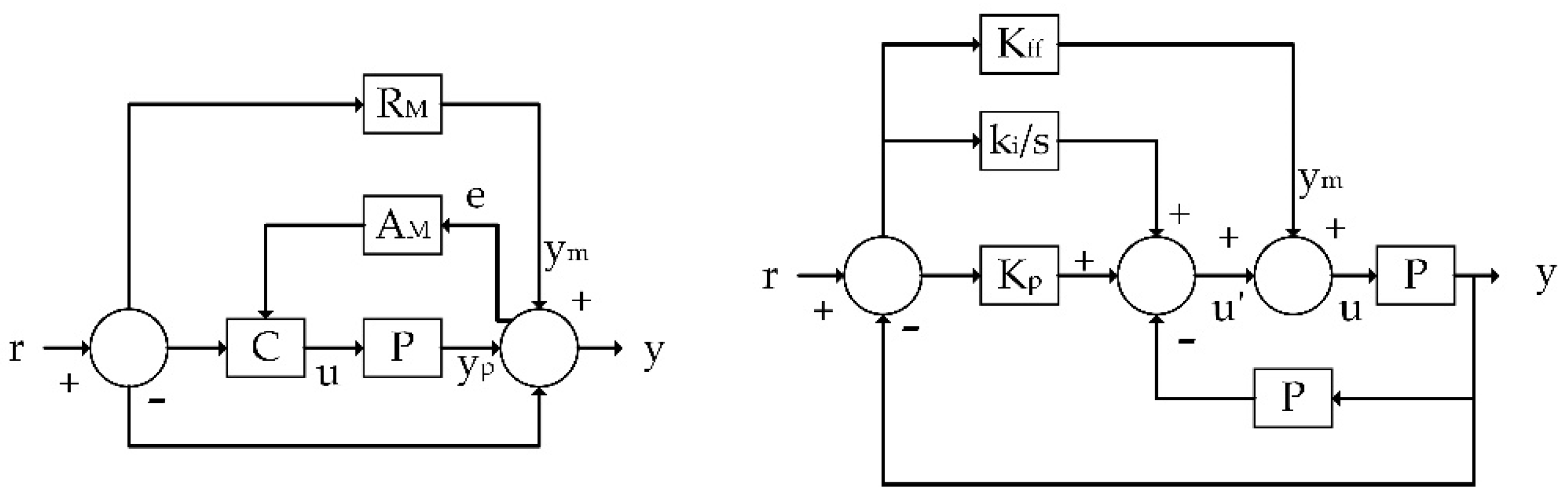
1.2. Proportional Integral Velocity Plus—Feed Forward Scheme (PIV-FF)

The schematic representation of the PIV-FF structure is outlined in Figure 2. The mathematical description of the PIV-FF structure is shown in Equation (3).

$$u=(K_p+\frac{K_i}{s})\left(r-y\right)-K_{v}r+K_{ff}r$$

(3)

where $K_p,K_i,\mathrm{and}{K}_v$ corresponds to proportional, integral, and velocity controller gains, respectively. $K_{ff}$ is the feed-forward gain of the system,$u,r$, and $y$ are control input, reference, and process output, respectively. However, in this control scheme, a tracking error with lag still exists.

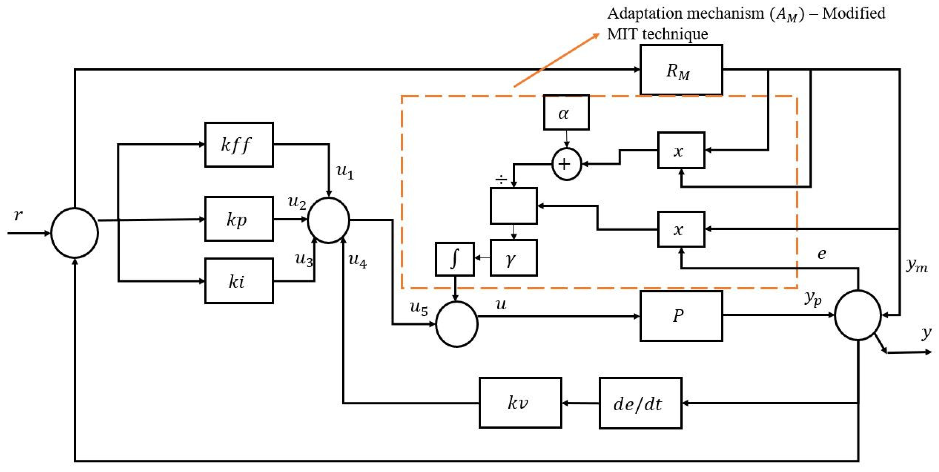
1.3. Enhanced MRAC Scheme

The MRAC scheme shown in Figure 3, in general, employs a P or PI or Proportional-Integral-Derivative (PID) control structure. In the Proportional-Integral-Derivative (PID) scheme, the parameters are tuned concerning the position error at that instant of time whereas, in PIV, the corrections are based on both the position and velocity error information. This makes the later performance more precise than the former scheme. Also, PIV is mostly preferred in motion control applications. In this study, PIV + FF is utilized as a control structure with a standard modified MIT adaptation mechanism and the performance analysis is carried out for the non-linear unstable MAGLEV system. The proposed enhanced MRAC control scheme consists of four gains, namely $K_p,K_i,K_v,\mathrm{and}{K}_{ff}$ and the adaptation mechanism consists of two tuning parameters, namely the adaptation rate $\left(\gamma \right)$ and amplification gain $\left(K_a\right)$. The controller gains $\left(K_p,K_i,K_v,\mathrm{and}{K}_{ff}\right)$ are evaluated by a direct comparison method where the closed-loop ball position characteristic equation is compared with the characteristic equation, which possesses the desired time domain specifications, which include mainly the overshoot $\left(M_p\right)$ and settling time $\left(t_s\right)$ parameters. The reference model $\left(R_M\right)$ is chosen following the expected behaviour of the system as time progresses. Proportional-Integral-Velocity (PIV) controllers are generally employed for precise motion control applications. However, this structure inherently produces some offset, which is compensated with a Feed-Forward (FF) controller. The capability to learn and adapt to the changes with the extra bounded condition imposed as a time-domain specification in PIV + FF makes MRAC into enhanced MRAC.

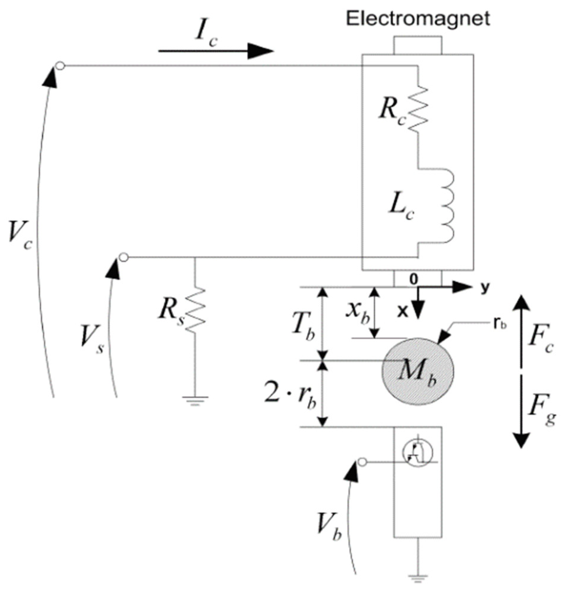
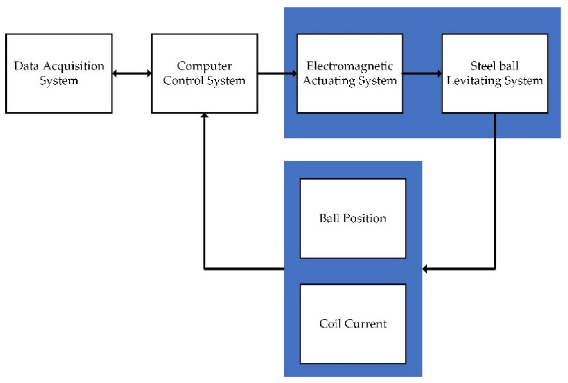
1.4. Mathematical Modeling of the Maglev System

The schematic representation of a MAGLEV system is shown in Figure 4. The plant parameters of the benchmark MAGLEV system used in this study are presented in

Table 1. Parameters of Maglev.

Symbol	Description	Value
Rc	Coil resistance	10 Ω
Lc	Coil inductance	412.5 mH
lc	Coil length	0.0825 m
rc	Coil steel core radius	0.008 m
Rs	Current sense resistance	1 Ω
rb	The radius of the ball	1.27 × 10−2 m
Mb	Mass of the ball	0.068 kg
Tb	Ball travel	0.014 m
G	Gravitational constant	9.81 m/s2
cmax	Maximum coil current	3 A
Kb	Ball position sensor sensitivity	2.83 × 10−3 m/V
Km	Electromagnet force constant	6.53 × 10−5 N.m2/A2

. The coil voltage $(V_c)$ supplied to the electromagnet can be obtained by applying Kirchhoff’s voltage law, as shown in Equation (4). The transfer function of the electromagnet can be obtained by using Equation (5).

$$V_c=\left(R_c{R}_s\right)I_c+L_c\frac{d}{dt}{I}_c$$

(4)

$$G_c\left(s\right)=\frac{I_c\left(s\right)}{V_c\left(s\right)}=\frac{K_c}{{\tau }_{c}s+1}$$

(5)

where $K_c$ is the static gain and ${\tau }_c$ is the time constant.

1.4.1. Equation for the Motion of the Ball

The attractive force acting on the ball due to the electromagnet is given by Equation (6).

$$F_c=\frac{K_m{I}_c{\left(t\right)}^2}{2x_b{\left(t\right)}^2}$$

(6)

where $x_b$ is the ball position and $K_m$ is the electromagnetic force constant. Similarly, the opposing force acting on the ball due to gravity is given by Equation (7). Hence, the total force experienced by the ball is given by Equation (8).

$$F_g=M_{b}g$$

(7)

$$F_{ext}=-F_c+F_g=-\frac{K_m{I}_c{\left(t\right)}^2}{2x_b{\left(t\right)}^2}+M_{b}g$$

(8)

Applying Newton’s second law, we can obtain the following nonlinear equation of motion (EOM) of the ball.

$$\ddot{ x_b}\left(t\right)=-\frac{K_m{I}_c{\left(t\right)}^2}{2M_b{x}_b{\left(t\right)}^2}+g$$

(9)

We can obtain the following transfer function of the magnetic levitation system about the equilibrium point $\left(x_{b0},I_{c0}\right)$ by linearizing Equation (9) using Taylor’s series.

$$G_b\left(s\right)=\frac{\Delta x_b\left(s\right)}{\Delta I_c\left(s\right)}=-\frac{K_b}{S^2-{\omega }_b^2}$$

(10)

where $K_b$ is the direct current gain and $w_b$ is the natural frequency in rad/s. Equation (1) represents the open-loop system, which is unstable. Hence, the maglev plant needs a feedback controller to stabilize the plant.

1.4.2. Controller Synthesis

The Maglev current $\left(I_c\right)$ to position $\left(x_b\right)$ the transfer function model is given by Equation (11).

$$G\left(s\right)= \frac{X_b\left(s\right)}{I_c\left(s\right)}=\frac{-2g{x}_{b0}}{I_{c0}{x}_{b0}\left(s^2-\frac{2g}{x_{b0}}\right)}$$

(11)

Equation (12) is substituted above to get the closed-loop structure.

$$I_c\left(s\right)=\left(K_p+\frac{K_i}{s}\right)\left(X_{b,d}\left(s\right)-X_b\left(s\right)\right)-K_v{X}_b\left(s\right)+K_{ff}{X}_{b,d}\left(s\right)$$

(12)

The closed-loop ball position control structure can be given by Equation (13).

$$T\left(s\right)=\frac{X_b\left(s\right)}{X_{b,d}\left(s\right)}=\frac{2g{x}_{b0}\left(K_{ff}+K_p\right)s+K_i}{-I_{c0}{x}_{b0}{s}^3+2x_{b0}g{K}_v{s}^2+\left(2x_{b0}g{K}_p+2I_{c0}g\right)s+2x_{bo}g{K}_i}$$

(13)

Time-domain specifications are defined for the dynamics of interest. To achieve 1-mm square wave position setpoint from the ball equilibrium position in mid-air, the ball position behaviour must satisfy the following design performance requirements of Percent Overshoot, less than 5%, no static steady-state error, ($e_{ss}=0$), maximum settling time less than 0.3 s, and minimized control effort produced, which is proportional to the coil input voltage $(V_c)$. The steel ball position behaviour is subjected to operate at an equilibrium point with peak overshoot $\left(M_p\right)$ less than 5% and a steady-state error $\left(e_{ss}\right)$ equal to zero with a minimum control effort and settling time $\left(t_s\right)$ of less than 0.3 s. The third-order system can be defined by Equation (14).

$$\left(s+p_0\right)\left(s^2+2\zeta {\omega }_{n}s+{\omega }_n^2\right)=s^3+\left(p_0+2\zeta {\omega }_n\right)s^2+\left(2p_0\zeta {\omega }_n+{\omega }_n^2\right)+p_0{\omega }_n^2$$

(14)

With natural frequency $({\omega }_n)$ of 19.3 rad/s, damping ration $\left(\zeta \right)$ of 0.69, and a pole $\left(p_0\right)$ at 40 rad/s, the desired time domain specifications can be met. The system is assumed to operate at a static equilibrium condition with $x_{b0}=6\mathrm{mm}$. At the equilibrium point, the weight of the ball equals the electromagnetic force. From Equation (9), we obtain the following.

$$I_{c0}=\sqrt{\frac{2M_{b}g}{K_m}}{x}_{b0}$$

(15)

Substituting the plant parameters from Table 1, and $x_{b0}$, $I_{c0}=0.86$. From Equation (12), at equilibrium $X_b=X_d=X_{b0}$, $I_c=I_{c0}$, we get Equation (16).

$$I_c=I_{c0}=K_{ff}{x}_{b0}$$

(16)

The feedforward gain $K_{ff}$ can be obtained as $K_{ff}=\frac{I_{c0}}{x_{b0}}$. Similarly, substituting all the plant parameters and the ${\omega }_n,\zeta ,p_0$ and equating with Equation (13), $K_p,K_i,\mathrm{and}{K}_v$ can be obtained. A First-order reference model is chosen on the assumption that the system will try to have no overshoot once the system has adapted completely during the study. Since the real-time MAGLEV system is nonlinear and sensitive to environmental disturbances like varying light intensity and wind, the learning rate parameter/adaptation mechanism will take care of the fluctuations in dynamics. Failing to which will make the steel ball jump out of the experimental setup, the learning rate parameter/adaptation mechanism will take care of the fluctuations in dynamics. In the MRAC scheme, these parameters are updated periodically with an adaptation mechanism. The reference model $\left(R_M\right)$ taken for analysis is given in Equation (17).

$$R_M=\left(\frac{k}{\tau s+p}\right)$$

(17)

The time constant $\left(\tau \right)$ is the parameter that determines the speed of response of the system. The system with less of a time constant will have a faster response time. The gain $\left(k\right)$ determines the final value of the system. The learning or adaptation rate ($\gamma )$ is the parameter that forces the processes toward convergence. This parameter is largely influenced by the magnitude of the input signal. For the tracking of a more complex pattern, the amplification gain $\left(K_a\right)$ is introduced into the process for providing faster convergence. It is found based on experimentation by various trials. The amplification gain $\left(K_a\right)$ is approximately four times the learning rate $\left(\gamma \right)$ for complex tracking patterns. For other standard test signal patterns, the amplification gain is chosen to be 1. However, the $\gamma$ is meant to be chosen according to the process input conditions as per Equation (18).

$$K_a\simeq \{\begin{array}{c}4\gamma ; \mathrm{for} \mathrm{complex} \mathrm{input} \mathrm{trajectory} \mathrm{tracking}\\ 1; \mathrm{for} \mathrm{simple} \mathrm{input} \mathrm{trajectory} \mathrm{tracking}\end{array}$$

(18)

The system is subjected to analysis by a varying learning rate $\left(\gamma \right)$ and the values of $K_v$ in the obtained range.

$$f_v=\frac{{\omega }_n^2}{s^2+2\zeta {\omega }_n+{\omega }_n^2}$$

(19)

The velocity portion of the control scheme $\left(k_v\right)$ is integrated with a derivative filter, as shown in Equation (19) to compensate for noise association during the processes.

2. Results

The proposed control scheme is validated for its performance on the standard benchmark MAGLEV system shown in Figure 1. The block diagram of the real-time experimentation setup is shown in Figure 5. The setup consists of a MAGLEV plant, a computer control system, a data acquisition board associated with a signal conditioning circuit, and the MAGLEV system parameters, which are presented in Table 1. The MAGLEV system consists of a current sensor and photo sensor for measuring coil current and ball position, respectively. The input range and resolution of Data Acquisition (DAQ) are ±10 V and 12 bits, which can measure signals up to a 2 kHz control rate. A power amplifier with a regulated supply of ±10 V at 3 A governs the current supplied to the electromagnet. The Quanser real-time control (QUARC) software is used for hardware in loop (HIL) testing. The control algorithm realized in Simulink interacts with the QUARC software. The controller parameters $K_p,K_i,K_v,\mathrm{and}{K}_{ff}$ are chosen to be $-199.7\frac{\mathrm{A}}{\mathrm{m}},-633.2\mathrm{A}/\mathrm{ms},$ $-2.82\frac{\mathrm{As}}{\mathrm{m}},$ and $138.6\frac{\mathrm{A}}{\mathrm{m}},$ respectively. The damping factor $\left(\zeta \right)$ and the natural frequency $\left({\omega }_n\right)$ are chosen to be 0.9 and −500 rad/s for experimentation. The first-order model is taken as the reference model for analysis.

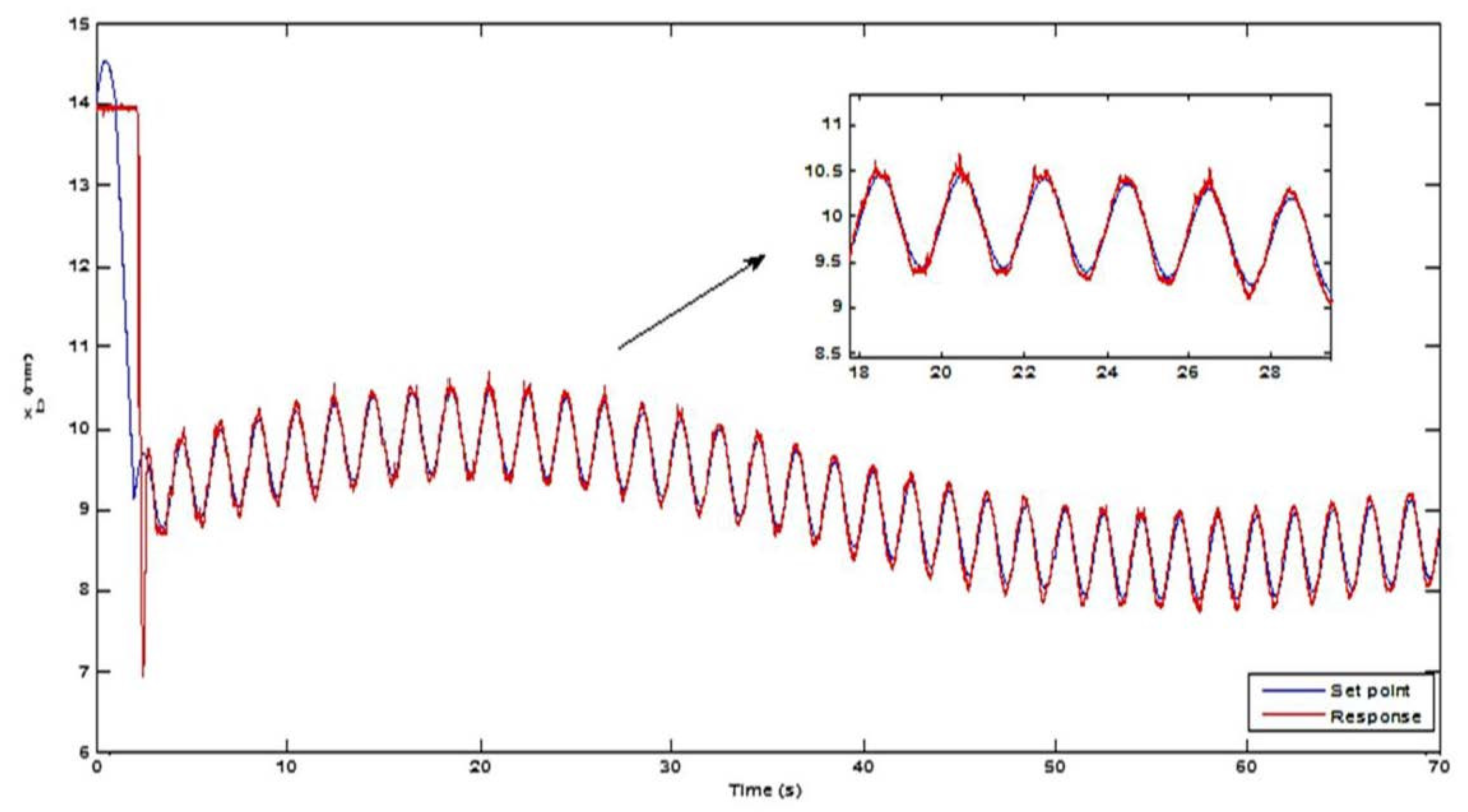
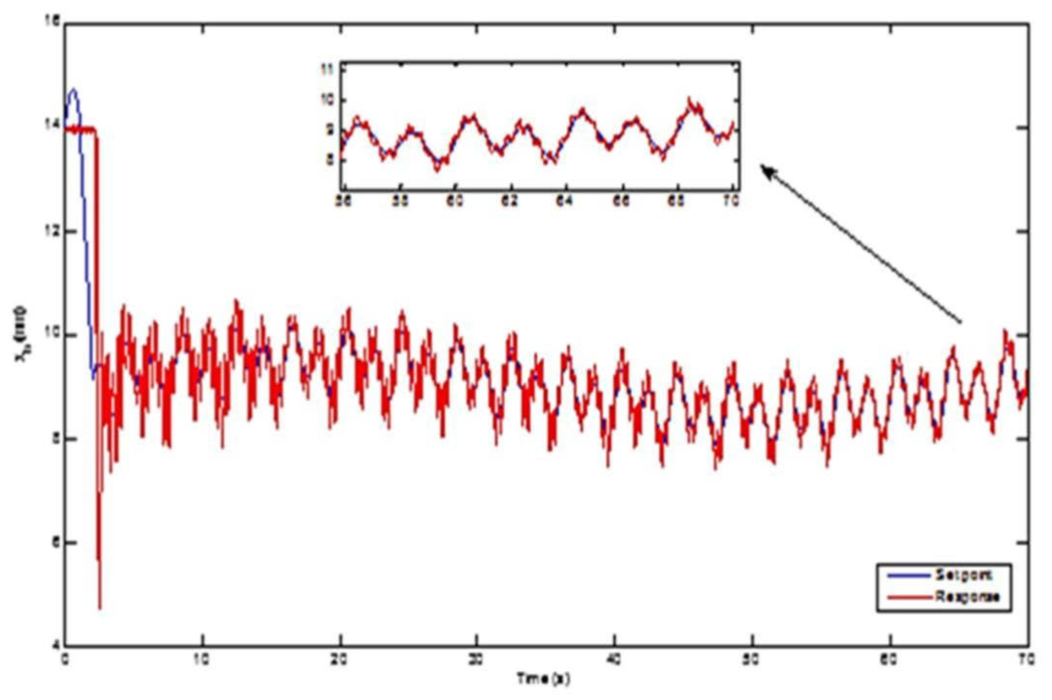
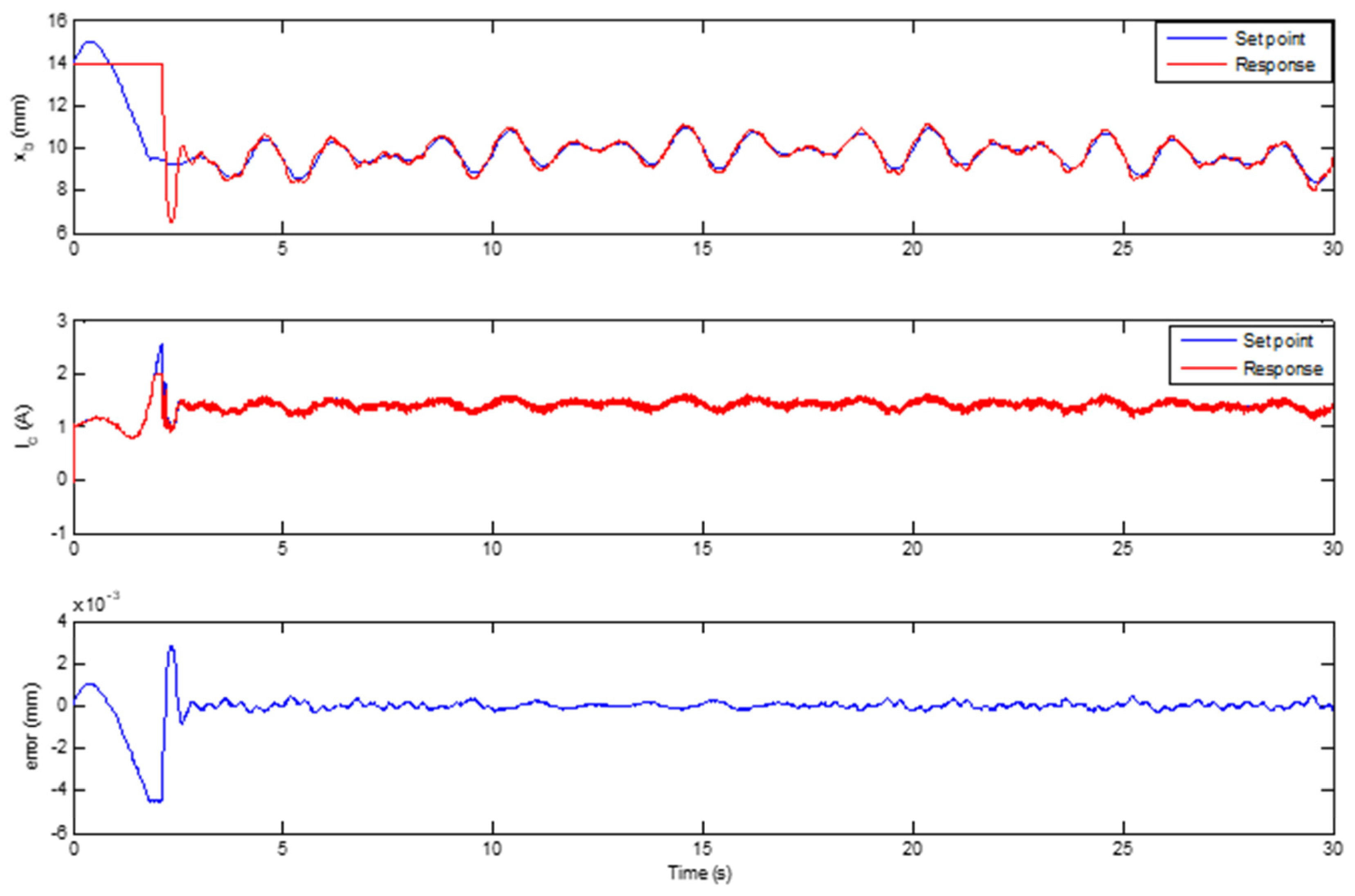
2.1. Multi-Sine Trajectory Tracking

The attractive force acting on the ball due to the electromagnet is given by Equation (6). The system is subjected to a performance analysis by applying highly asymmetric, complicated input patterns. The system responds and adapts to the most intricate input patterns. The combination of sinusoidal inputs was taken for achieving the asymmetric patterns. The input patterns used for analysis can be mathematically described in Equation (20).

$$r\left(t\right)=T_b\left(x_{bo}u\left(t\right)+xsin\left(f_{x}t\right)+ysin\left(f_{y}t\right)+zsin\left(f_{z}t\right)\right)$$

(20)

where $x_{b0}$ is the equilibrium operating point applied with a step test signal in combination with multiple sine inputs with magnitude $x,y,\mathrm{and}z$ and frequency $f_x,f_{y,}\mathrm{and}{f}_z,$ respectively, with a bias of $T_b$. Three different set cases have been taken for analysis with the above-described input model. The results are listed as individual cases below. The input pattern with $x$, $y$, and $z$ as 0.5, 0.5, and 0.5 mm magnitude respectively and $f_x$, $f_y$, and $f_z$ as 0.015 Hz, 0.01 Hz, and 0.5 Hz, respectively, is used for case 1 analysis. The first-order model is used as the reference model whose general form is denoted in Equation (17) for analyzing the behaviour of the system. The experimentation is carried for 30 s and the ball position tracking is shown in Figure 6. The input pattern with $x$, $y$, and $z$ as 0.5, 0.25, and 0.5 mm magnitude respectively and $f_x,f_y,\mathrm{and}{f}_z$ as 0.15 Hz, 0.25 Hz, and 0.5 Hz, respectively, is used for case 2 analysis.

The input pattern with $x,y,\mathrm{and}z$ as 0.5, 0.25, and 0.5 mm magnitude respectively and $f_x,f_y,\mathrm{and}{f}_z$ as 0.15 Hz, 0.25 Hz, and 0.5 Hz, respectively, is used for case 2 analysis. All these analyses are carried out with $x_{b0}=6\mathrm{mm}$ and $T_b$ = 0.014 mm. The system is applied with adaptation gain $\left(\gamma \right)$ as −10 and amplification gain $\left(K_a\right)$ to be 40 (refer (18)). It is inferred from the plots of Figure 7 that, as the complexity in pattern keeps increasing concerning its change in input signals magnitude and frequency, the system performance is varied. This is mainly because of the learning rate $\left(\gamma \right)$ used during the process. The adaptation or learning rate largely depend on the magnitude of the input. By changing $\gamma =-7$, the variation in the tracking performance is observed.

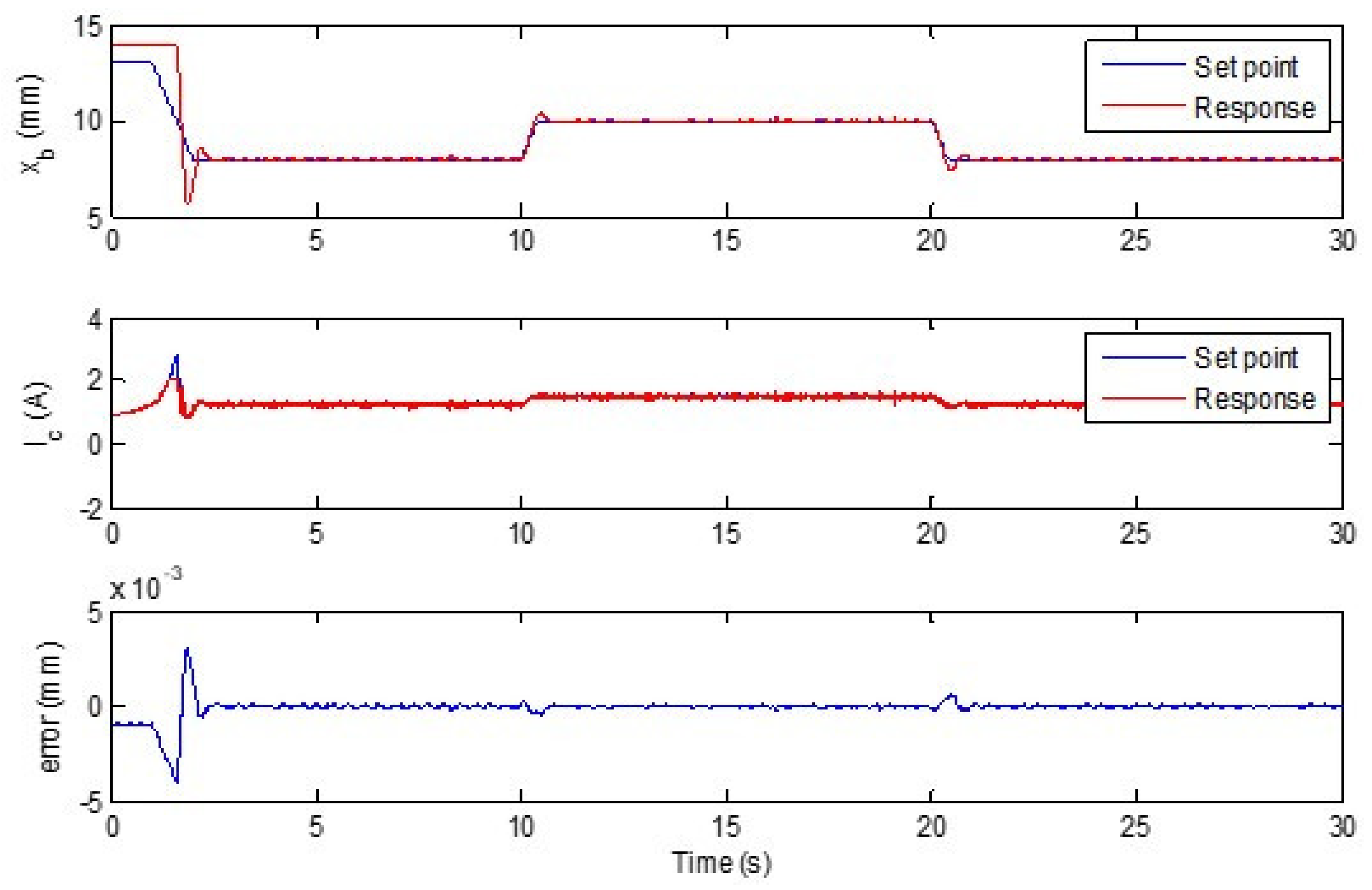
2.2. Symmetric Trajectory Tracking

The symmetric rectangular trajectory with an initial step is applied for analyzing the system response. The input with a rectangular function is described with a magnitude of 1 and a frequency of 0.05 Hz. Figure 8 shows the ball position tracking with coil current, the control effort, and the error, respectively. The experimentation is carried out with a period of 30 s. It could be observed from the response that the system tracks effectively, and it converges to the desired trajectory without much delay. The system is provided with an adaptation gain $\left(\gamma \right)$ of −10 with the amplification gain $\left(K_a\right)$ of $40$. The first-order model with $\tau =1\mathrm{ms}$, $p=10$ used as the reference model (refer (17)) for the system to attain the desired characteristics.

3. Discussion

The Enhanced MRAC scheme response is compared with the conventional PIV+FF system and the performance can be visualized from Figure 9. The Root Mean Square Error (RMSE) value is computed for both the control schemes. It is found that the values for PIV + FF are 0.2968 mm and for Enhanced MRAC is 0.2913 mm, respectively. Figure 10 illustrates the Power Spectral Density (PSD) of the ball tracking by the PIV + FF controller and the MRAC-PIV + FF controller scheme. It can be inferred that the later produces lesser PSD than the former.

4. Conclusions

The Enhanced MRAC scheme is applied to the MAGLEV system and the performance is tested by applying different input trajectory patterns, such as multi-sine and square wave patterns. The relation between the learning rate and amplification gain was framed through various trials and errors for good tracking performance of the complicated signal. It is inferred through experiments that the learning rate largely influences the faster system convergence of the system. The performance evaluation is carried with RMSE and PSD. The experimental results elucidate that the Enhanced MRAC adapts well to the changes and provides good tracking capability. As future work, analysis can be extended to a different reference model as per the requirement along with the suitable choice of the learning rate parameter. The influence of amplification gain to the reference model and learning rate could be analyzed. The adaptation mechanism can be made heuristic and the performance of the tracking could be analyzed with the same PIV+FF control scheme.

References

1. Charara, A.; De Miras, J.; Caron, B. Nonlinear control of a magnetic levitation system without premagnetization. IEEE Trans. Control. Syst. Technol. 1996, 4, 513–523. [Google Scholar] [CrossRef]
2. Yaseen, M.H.; Abd, H.J. Modeling and control for a magnetic levitation system based on SIMLAB platform in real time. Results Phys. 2018, 8, 153–159. [Google Scholar] [CrossRef]
3. Tuan, T.A.; Suzuki, S.; Sakamoto, N. Nonlinear optimal control design considering a class of system constraints with validation on a magnetic levitation system. IEEE Control Syst. Lett. 2017, 2, 418–423. [Google Scholar]
4. Krzysztof, K.; Mitura, A.; Lenci, S.; Warminski, J. Energy harvesting from a magnetic levitation sys-tem. Int. J. Non-Linear Mech. 2017, 94, 200–206. [Google Scholar]
5. Kim, S.-K.; Ahn, C.K. Variable Cut-Off Frequency Algorithm-Based Nonlinear Position Controller for Magnetic Levitation System Applications. IEEE Trans. Syst. Man, Cybern. Syst. 2019, 1–7. [Google Scholar] [CrossRef]
6. Chen, C.; Xu, J.; Ji, W.; Rong, L.; Lin, G. Sliding Mode Robust Adaptive Control of Maglev Vehicle’s Nonlinear Suspension System Based on Flexible Track: Design and Experiment. IEEE Access 2019, 7, 41874–41884. [Google Scholar] [CrossRef]
7. Gao, Y.; Wang, Y.; Zhang, J.; Li, M.; Yue, Q.; Zhang, W. A sliding mode periodic adaptive learning operation control method for medium-speed maglev trains. In Proceedings of the 2020 39th Chinese Control Conference (CCC), Shenyang, China, 27–29 July 2020; pp. 5548–5553. [Google Scholar]
8. Kim, C.-H. Robust Control of Magnetic Levitation Systems Considering Disturbance Force by LSM Propulsion Systems. IEEE Trans. Magn. 2017, 53, 1–5. [Google Scholar] [CrossRef]
9. Yang, Z.; Pedersen, G. Automatic Tuning of PID Controller for a 1-D Levitation System Using a Genetic Algorithm—A Real Case Study. IEEE Int. Symp. Intell. Control 2006, 3098–3103. [Google Scholar] [CrossRef]
10. Sivrioglu, S.; Basaran, S.; Yildiz, A.S. Multisurface HTS-PM Levitation for a Flywheel System. IEEE Trans. Appl. Supercond. 2016, 26, 1–6. [Google Scholar] [CrossRef]
11. Rahul, S.G.; Dhivyasri, P.G.; Kavitha, S.; Arungalai, V.K.A.; Kumar, R.; Garg, A.; Gao, L. Model refer-ence adaptive controller for enhancing depth of penetration and bead width during cold metal transfer joining process. Ro-Botics Comput.-Integr. Manuf. 2018, 53, 122–134. [Google Scholar] [CrossRef]
12. Garza, L.E.; Castanon, A. Vargas Martinez and R. Cruz Reynoso, “MRAC-based Fault Tolerant Control of a SISO Real Pro-cess Application. IEEE Lat. Am. Trans. 2015, 13, 2545–2550. [Google Scholar] [CrossRef]
13. Espinoza, A.T.; Sanchez, W. On-board parameter learning using a model reference adaptive position and attitude con-troller. In Proceedings of the 2017 IEEE Aerospace Conference, Big Sky, MT, USA, 3–11 March 2017. [Google Scholar]
14. Pawar, R.J.; Parvat, B. Design and implementation of MRAC and modified MRAC technique for inverted pendulum. In Proceedings of the 2015 International Conference on Pervasive Computing (ICPC), Pune, India, 8–10 January 2015; pp. 1–6. [Google Scholar]
15. Balko, P.; Rosinova, D. Modeling of magnetic levitation system. In Proceedings of the 2017 21st International Conference on Process Control (PC), Štrbské Pleso, Slovakia, 6–9 June 2017; pp. 252–257. [Google Scholar]
16. Deshan, K.; Dong, J.; Yanchao, Z.; Xukun, L.; Deyu, W. Research on rejection magnetic levitation model simulation and wavelet analysis of its signal. In Proceedings of the 2019 14th IEEE International Conference on Electronic Measurement & Instruments (ICEMI), Changsha, China, 1–3 November 2019; pp. 1701–1707. [Google Scholar]
Figure 1. Magnetic levitation system.
Energies 14 01455 g001
Figure 2. Model Reference Adaptive Control Scheme (left) PIV-FF scheme (right).
Energies 14 01455 g002
Figure 3. Enhanced Model Reference Adaptive Control (EMRAC) Scheme.
Energies 14 01455 g003
Figure 4. Schematic of the Magnetic Levitation System.
Energies 14 01455 g004
Figure 5. Block diagram of the Magnetic Levitation (MAGLEV) system.
Energies 14 01455 g005
Figure 6. (Top) Multi-sine pattern—Case 1, (bottom) and Multi-sine pattern—Case 2.
Energies 14 01455 g006aEnergies 14 01455 g006b
Figure 7. Multi-sine pattern—case 3 analysis.
Energies 14 01455 g007
Figure 8. Symmetric tracking pattern.
Energies 14 01455 g008
Figure 9. Performance validation.
Energies 14 01455 g009
Figure 10. Power spectral density of PIV+FF and MRAC-PIV+FF.
Energies 14 01455 g010