Article

Simplified Transition and Turbulence Modeling for Oscillatory Pipe Flows

Faculty of Mechanical Engineering, Technion—Israel Institute of Technology, Technion City, Haifa 320003, Israel
*
Author to whom correspondence should be addressed.
Energies 2021, 14(5), 1410; https://doi.org/10.3390/en14051410
Submission received: 14 January 2021 / Revised: 15 February 2021 / Accepted: 25 February 2021 / Published: 4 March 2021
(This article belongs to the Special Issue Turbulence and Fluid Mechanics)

Abstract

:
One-dimensional unsteady Reynolds-averaged Navier–Stokes computations were performed for oscillatory transitional and turbulent pipe flows and the results were validated against existing experimental data for a wide variety of oscillatory Reynolds and Womersley numbers. An unsteady version of the Johnson–King model was implemented with optional near-wall modification to account for temporal pressure gradient variations, and the predictions were compared with those of the Spalart–Allmaras and kε turbulence models. Transition and relaminarization were based on empirical Womersley number correlations and assumed to occur instantaneously: in the former case, this assumption was valid, but in the latter case, deviations between data and predictions were observed. In flows where the oscillatory Reynolds numbers are substantially higher than the commonly accepted steady critical value (~2000), fully or continuously turbulent models produced the best correspondence with experimental data. Critically and conditionally turbulent models produced slightly inferior correspondence, and no significant benefit was observed when near-wall pressure gradient effects were implemented or when common one- and two-equation turbulence models were employed. The turbulent velocity profiles were mainly unaffected by the oscillations and this was explained by noting that the turbulent viscosity is significantly higher than its laminar counterpart. Thus, a turbulent Womersley number was proposed for the analysis and categorization of oscillatory pipe flows.

1. Introduction

Oscillating pipe flows with zero net flowrates are common in engineering systems and particularly in Stirling-based engines and heat pumps, e.g., pulse-tube cryogenic coolers [1,2,3]. Oscillatory Reynolds numbers ( R e o s U o s 2 a / ν ) can be on the order of hundreds or thousands [1,3] in small devices and well over 106 for large-scale devices (e.g., Wollan et al. [4]). A central challenge in modeling these systems is that the Reynolds number varies greatly within the cycle, often crossing from laminar to turbulent flow regimes [5]. When Reynolds numbers are super-critical, the flow can undergo both laminar–turbulent and turbulent–laminar transitions; the latter is sometimes referred to as relaminarization (Narasimha and Sreenivasan [6]). Contrary to a steady flow in which the transition between the laminar and the turbulent regimes is determined only by the Reynolds number, for oscillating flow, the transition is determined empirically by a combination of the peak oscillatory Reynolds number Reos and a dimensionless frequency. Typically, a Stokes parameter λ a ω / 2 ν or, more commonly, the Womersley number α a ω / ν is used. A compendium of results from different investigations is presented in the detailed and extensive review by Çarpınlıoğlu and Özahi [7].
Sergeev [8] performed a pioneering investigation and found that frequency has a significant effect on transition, expressed as R e o s , crit = k α , where k = 710 within the 4 α 40 range. Subsequent investigations produced similar correlations. Experiments were performed by Hino et al. [5] at Reos ≤ 5830, and they classified the flow into three different flow regimes on a characteristic diagram (Reos versus α map, see Figure 1), namely, laminar and distorted laminar flows, weakly turbulent flows, and conditionally turbulent flows. Distorted laminar flows are characterized by amplitude perturbations that appear in the early stage of the accelerating phases ( d | U | / d t > 0 ) in the central portion of a pipe. In weakly turbulent flows small perturbations are observed during the portion of the phase that corresponds to higher velocities, while conditionally turbulent flows are characterized by turbulent bursts that occur during flow deceleration ( d | U | / d t < 0 ). Ohmi et al. [9] performed a similar series of experiments at Reos = 64,500 and recognized the existence of a critically turbulent regime, where turbulent bursts occur in the accelerating phase and in the decelerating phase. No reliable correlation for the transition between the conditionally and critically turbulent regimes was determined.
On the basis of their extensive review, Çarpınlıoğlu and Özahi [7] concluded that the mean value of the constant k is 750 and is accurate to within 12%. Çarpınlıoğlu and Özahi [7] calculated the average value of no less than seven investigations, namely, Segeev [8], Hino et al. [5], Ohmi et al. [9], Ohmi and Iguchi [10], Eckmann and Grotberg [11], Akhavan et al. [12], and Das and Arakeri [13]. Exceptions to this are the investigation of Merkli and Thomann [14] and Zhao and Cheng [15] who reported values between 380 and 400. Experiments at significantly higher Reynolds numbers (Reos = 220,000 at α = 75) were reported by Lodahl et al. [16], who also considered a mean flow superimposed on the oscillations. Instead of imposing a harmonic bulk flow, Lodahl et al. [16] imposed a harmonic centerline velocity for their experiments. The experiment of Hino et al. [5] at Reos = 5830 and α = 2.70 (see Figure 1) is of particular interest because it shows both critically and conditionally turbulent regimes within the same experiment (see discussion in Section 3.1). As such, it can be considered to lie on the boundary between the two regimes.
Ahn and Ibrahim [17] performed computations using a high Reynolds number kε turbulence model and showed a significant phase mismatch. Walther et al. [18] also used a low-Reynolds-number kε model to investigate heat transfer in the turbulent oscillating pipe flow. They developed a correlation for the Nusselt number but did not compare their turbulent model with experimental results. Feldman and Wagner [19,20] performed direct numerical simulations (DNS) of fully developed oscillating turbulent pipe flow. The authors pointed out that relatively few DNS studies have been conducted due to the significant computational costs. Hanjalić et al. [21] applied their model to a pipe flow case of Hino et al. [5] and observed a qualitative agreement with data. Experiments on boundary layers of this type are difficult to conduct and thus investigators compare their results to data acquired in rectangular and square channel flows (e.g., [22,23,24]. More recently, Ghodke and Apte [25,26] performed particle-resolved direct numerical simulations (DNS) for the purpose of investigating the behavior of an oscillatory flow field over rough surfaces.
The global objective of this research was to develop simplified transition and turbulence models for oscillatory pipe flows corresponding to the different flow regimes on the characteristic diagram (Figure 1). A simplified approach was adopted here, primarily for the purposes of performing rapid calculations within the framework of a suite of Stirling engine and pulse-tube design codes. To achieve this, a numerical scheme was developed to solve the fully developed time-dependent Reynolds-averaged Navier–Stokes equations. The code was verified against cases where analytical and semi-empirical solutions exist. Subsequently, computations were performed for a wide range of oscillatory Reynolds and Womersley numbers, and validated against available experimental data.

2. Modeling Methods and Rationale

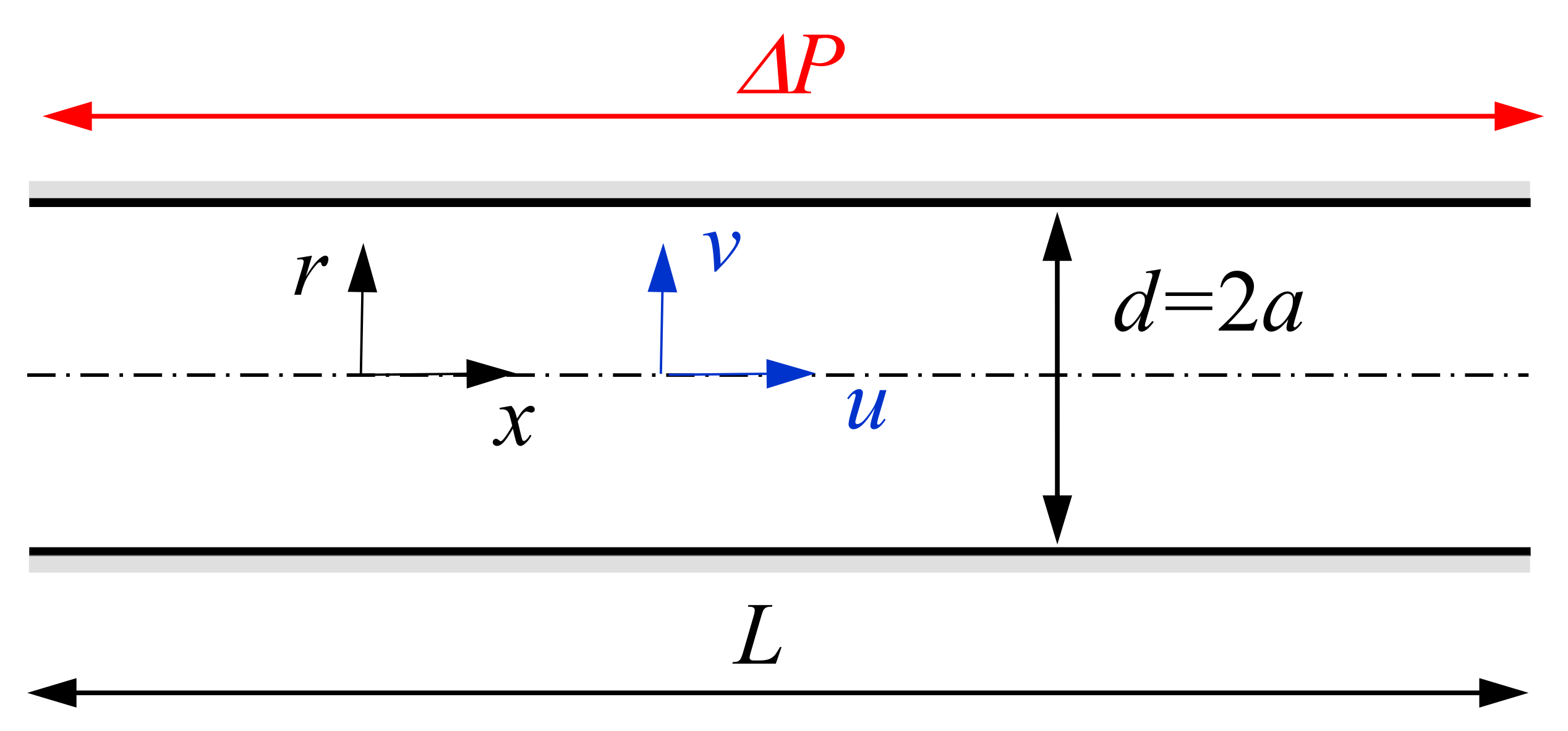
For purposes of modeling the flow, we adopt a pipe whose coordinates in the radial and streamwise directions are r and x; its radius and length are designated a and L. Figure 2 shows a schematic of the problem. The flow is assumed to be turbulent, fully developed in the x-direction, incompressible, and with constant density ρ. The phase-averaged axial and radial velocities u and v , respectively, and P is the phase-averaged pressure. It is subjected to an oscillating pressure difference ∆P, resulting in a pressure gradient d P ( t ) / d x = Δ P ( t ) / L .
For the computational results presented in this paper, two different numerical approaches were adopted. In both, the unsteady Reynolds-averaged Navier–Stokes (URANS) equations were solved, where “averaged” implies phase-averaging. In the first approach, the well-known unsteady one-dimensional momentum equation was solved and in the second approach, the well-known commercial software package: Fluent (Release 12.0, Ansys, Canonsburg, PA, USA) was employed. Section 2.1, Section 2.2, Section 2.3 and Section 2.4 describe the one-dimensional computations and Section 2.5 describes the computations conducted with Fluent.

2.1. Mass Conservation

Here we employ the integral form of the continuity equation, expressing the bulk volumetric flowrate as
Q ( t ) = U ( t ) π a 2
where U(t) is the phase-averaged cross-sectional (bulk) velocity. This integral form is used to check that Q(t), integrated over a period, is zero and guides us in the choice of turbulence models. To understand this, consider a harmonic mean flow imposed on the flow, common in many experiments, namely,
U t = U o s exp ( i ω t )
The fundamental phase-averaged local velocity, as reported in experiments, can be expressed as
u 0 r , t = u o s ( r ) exp i ω t Φ ( r )
If we assume that the velocity harmonics are negligible, then the volumetric flowrate is
Q ( t ) = 2 π 0 a r u 0 r , t d r
which can be expressed as
Q ( t ) = 2 π 0 a r   u o s ( r ) exp i ω t Φ ( r ) d r
from Equation (3). Substituting Equations (2) and (5) into Equation (1) and simplifying, results in the following mass conservation expression:
2 π a 2 U o s 0 a r u o s ( r ) exp [ i Φ ( r ) ] d r = 1
The integrand expressed in Equation (6) clearly shows the increased relative importance of accurate near-wall turbulence modeling [27]. Due to the axisymmetric nature of the problem, the mass conservation integrand is weighted by the radial distance; thus, accurate modeling of the near-wall region assumes greater importance than that near the center of the pipe, or core flow region. Equation (6) shows, for example, that an amplitude over-prediction in the near-wall region must be balanced by an under-prediction in the core region in order to satisfy mass conservation. Therefore, failure to adequately model the viscous sub-layer will also have a detrimental effect on the predictions of the core flow. Despite the increased relative importance of near-wall modeling, a superior outer flow model that better represents the phase-lag would also affect the near-wall prediction in a reciprocal manner. In an attempt to evaluate the above arguments, both relatively simple and higher-order models turbulence models are considered here.
The well-known unsteady one-dimensional momentum equation in the x-direction is
u r , t t = 1 ρ d P d x + 1 r r r ν + ν t r , t u r , t r
where ν t is the turbulent kinematic viscosity and the common Boussinesq assumption for the phase-averaged Reynolds stresses u v ( r , t ) = ν t ( r , t ) u ( r , t ) / r is employed. The nomenclature   is used to denote phase-averaging of the fluctuating velocity components. Equation (7) is subjected to the well-known no-slip and symmetry boundary conditions, which are
u = 0   at   r = a
u / r = 0   at   r = 0
The imposition of the axial pressure gradient and/or bulk velocity boundary conditions are described in Section 2.4.

2.2. Turbulence Modeling

The unsteady Johnson–King model [27,28] employed here incorporates both equilibrium and non-equilibrium modeling ideas and expresses the equilibrium eddy viscosity distribution as
ν t i , e q = D 2 κ y ( u v ) max , e q 1 / 2
ν t o , e q = β a u τ
ν t , e q = ν t o , e q 1 exp ( ν t i , e q / ν t o , e q )
where κ is the von Kármán constant (0.4), β is an outer-layer constant (0.08), the subscript “max” indicates the location at which the turbulent kinetic energy is at its maximum, and
D = 1 exp ( y u τ / ν A + )
is the van Driest damping term with the nominal value A + = 15 . The subscripts i and o refer to the inner and outer layers, respectively. In a similar fashion to the relationship introduced above, the non-equilibrium inner-layer eddy viscosity is given by ν t i = D 2 κ y ( u v ) max 1 / 2 , while that in the outer layer is determined by satisfying the relationship: ν t , max = ( u v ) max ( u / y ) max with ν t = ν t o 1 exp ( ν t i / ν t o ) . To utilize this model an equation is required for the velocity-scale ( u v ) max 1 / 2 g 1 and has the following form:
d g d t = a 1 l m , max 1 g g e q
where a1 = 0.05 and
l m , max / a = 0.14 1 0.08 y / a max 2 1 0.06 y / a max 4
Given the relatively poor predictions of standard and low Reynolds number turbulence models for both oscillatory and pulsatile flows and the demonstrated superior performance of the modified unsteady Johnson–King model [27], this model was used initially. Preliminary computation showed, however, that modeling of the non-equilibrium Reynolds stresses had only a minor effect on the computed results, whereas near-wall modeling, transition, and relaminarization modeling produced some differences. To this end, the equilibrium form of the Johnson–King model was used in combination with the near-wall model of Mao and Hanratty [29]. In addition, equilibrium-based (mixing-length) models and the popular Spalart–Allmaras [30] and the kε models were employed. An additional advantage of these models is that the effects of pressure gradient on the laminar sub-layer can be modeled or modified via the Van Driest parameter (A+) if this is desired.
Mao and Hanratty [29] suggested a correction that accounts for variable near-wall damping effects in unsteady pipe flows. Employing an analogy with steady flows, they proposed a variable Van Driest parameter as a function of the dimensionless pressure gradient as follows:
A + = A 0 + 1 + k 1 p eff +
where A 0 + and k 1 are constants (15 and −40, respectively). Furthermore, the dimensionless pressure gradient p eff + is calculated by solving the first-order lag equation:
d p eff + d t + = p + p eff + k L
where the constant k L = 220 . p + and t + are dimensionless pressure gradient and time, namely,
p + = ν ρ u τ 3 d P d x
and
t + = t u τ 2 / ν
The original model of Mao and Hanratty [29], with kL = 200, was proposed for small-amplitude pulsating flows that exhibited a linear response. Greenblatt [27] used this model for large-amplitude (65%) pulsating flows with the slightly modified constant above (kL = 220), and it produced satisfactory correspondence with experimental data. Nevertheless, there is some uncertainty when employing this constant for oscillatory flows and in order to evaluate this, we performed computations both with and without variable near-wall damping (see Section 3.2). The momentum Equation (7) was solved by means of a Crank–Nicolson second-order-accurate finite-difference numerical scheme. The computational grid was constructed with an enhanced grid density in the near-wall region, based on the compound interest formula. A total of 120 grid points were used in the radial direction, while a fixed time step was chosen to be equivalent to 500 timesteps per cycle. At the highest Reynolds number, the closest point to the wall fulfilled the condition y + < 1 . Implementation of the Crank–Nicolson scheme with variable grid density follows the approach taken by Greenblatt [27]. The numerical code was validated on the basis of comparisons with analytical solutions for oscillatory laminar flows [31] and established semi-empirical turbulent-flow laws.
The comparison between the calculations and the experimental results was performed relative to the amplitude ratio and the phase shift. These quantities were defined as properties of the fundamental wave of the Fourier transform, by means of the following relations:
U t = 2 a 2 0 a u r , t r d r
A r = max FFT u r , t max FFT U t
Φ r = max FFT u r , t max FFT U t
The solution was considered to be converged when there was a negligible difference between successive cycles. This was achieved by requiring that the relative change in cross-sectional phase-averaged velocity at each phase during successive cycles was less than 10−4 for both amplitude ratios and phase angles (in radians). Typically, convergence was achieved after five to six cycles. The above definitions (Equations (16)–(18)) were employed in order to remain consistent with, and facilitate a comparison with, experimental data. Within a converged cycle, Equation (17) represents the peak value in the Fourier transform of each local phase-averaged axial velocity divided by the corresponding value of the cross-sectional phase-averaged velocity. Equation (18) represents the difference between the respective corresponding phase angles.

2.3. Transition and Relaminarization Modeling

The challenge presented here was to render an appropriate model of each of the different flow regimes. The laminar regimes were straightforward; therefore, attention was focused on the conditionally turbulent and critically turbulent regimes (see Figure 1), and the turbulent state itself. In the conditionally turbulent flow, the transition occurs during the deceleration phase of the flow and when the oscillating Reynolds number exceeds its critical value; thus, two conditions must be fulfilled, namely, R e o s , crit k α and d | U | / d t < 0 . For the critically turbulent regime, transition occurs at supercritical Reynolds numbers during flow acceleration; thus, only the condition R e o s , crit k α must be fulfilled. Finally, for fully turbulent flow or continuously turbulent flow, the flow is assumed to be continuously turbulent without transition or relaminarization. Due to the lack of a credible transition model in unsteady flows, we assume that transition occurs instantaneously. This can be considered as a simple heuristic model as it is consistent with experimental data [5,9]. Implementation of these models was achieved by “initiating” or “terminating” the mixing-length term, and hence the eddy viscosity described below.

2.4. Enforcing Harmonic Average Bulk Flow

Experimental data are generated by imposing a harmonic or nearly harmonic oscillation of the bulk velocity U(t) or the centerline velocity. However, the momentum equation as formulated in this study requires the imposition of a time-dependent pressure gradient. For laminar and fully turbulent flows, a harmonically varying pressure gradient term results in a harmonic or close-to-harmonic average flow oscillation, respectively. However, for conditionally or critically turbulent models, the computations switch between laminar and turbulent solutions, and thus a harmonically varying pressure gradient can produce large higher harmonics of the average flow. To address this problem, the pressure gradient was varied iteratively at each time step in order to enforce a harmonically varying average flow. This was achieved by means of a simple bisection method where a criterion of 0.05% between calculated and harmonic bulk velocity was employed. The authors have not encountered this approach before, and the results will be discussed further in Section 3. In contrast to experiments, direct numerical simulations have been performed by imposing a harmonically varying pressure gradient on the pipe flow [19,20]. The phase-averaged results of such simulations can be very useful in the development of turbulence models.

2.5. Two-Dimensional Unsteady Computations

The two-dimensional unsteady computations were performed using Fluent, which is a finite-volume code with a pressure-based solver for incompressible flows. Temporal discretization is treated implicitly with a dual time step approach for unsteady calculations. The turbulent flow was modeled using (a) the Spalart–Allmaras turbulence model, (b) the kε model, and (c) the equilibrium version of the Johnson–King model described in Section 2.2. The Spalart–Allmaras model is a one-equation model that solves a modeled transport equation for νt, while the kε model solves transport equations for k and ε that are used to determine νt. The standard version of the kε model was used together with non-equilibrium wall-functions that include pressure gradient effects. The equilibrium form of the Johnson–King model was implemented via Fluent’s User Defined Function tool, which supports user-defined expressions for νt.
The main difference between these computations and those described above is that a finite-length pipe was employed, with L/d = 300 as the computational domain. This large L/d was employed to eliminate entrance effects [32], and the results presented here were extracted from the midpoint L/d = 150. The computational grid in the radial direction was identical to that described in Section 2.3 with 120 grid points, and 6000 points in the axial direction giving x + = 50 . Halving the grid density using 60 cross-stream points and 3000 streamwise points resulted in negligible differences to the computed values. The working fluid was selected air as an ideal gas. Moreover, a fixed time step was chosen to be equivalent to 500 timesteps per cycle. The convergence criterion was set to be the same as for the solution with the Crank–Nicolson scheme, namely, 10−4 for both the amplitude ratios for phase angle (in radians).

3. Computational Results

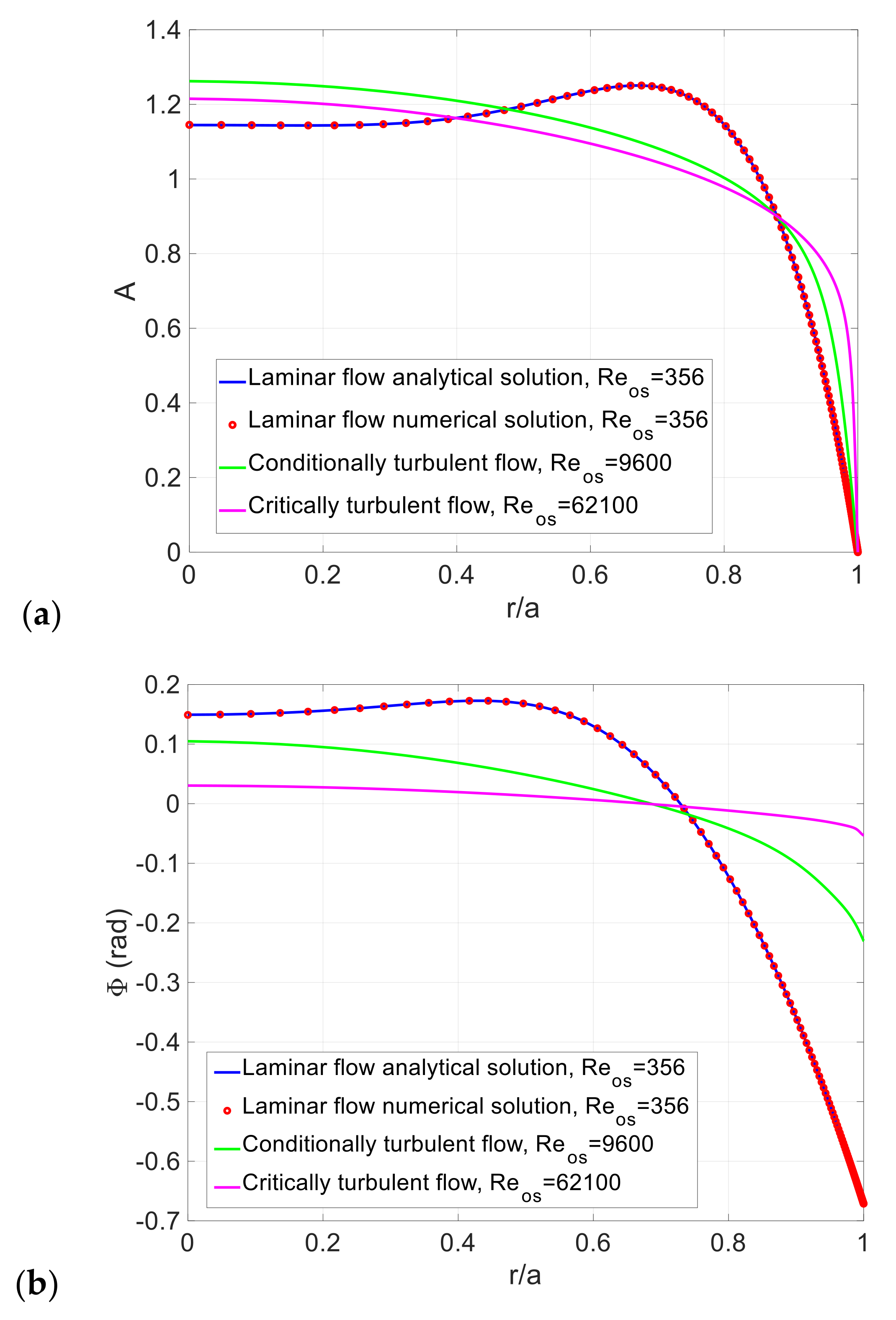
Validation of the numerical method and turbulence models for the different representative cases are presented in Figure 3a,b. For all cases, α = 10 . For the laminar flow, the numerical results show excellent correspondence with the analytical solution. For purposes of illustration, computations are also presented in Figure 3a,b for two different transition models, corresponding to critically and conditionally turbulent flows. Close to the wall, results of the conditionally turbulent computations exceed their laminar counterpart as a result of increased near-wall turbulent viscosity. However, in order to maintain mass conservation, the conditionally turbulent solution exhibits a lower amplitude in the approximate range 0.47 ≤ r/a ≤ 0.87 and a higher one for r/a < 0.47. With increasing Reynolds number and critically turbulent computations, the velocity profile amplitude tends toward a conventional turbulent profile. For the turbulent flows, the phase lag near the wall decreases substantially. With increasing Reynolds numbers, as expected, the profiles tend continuously toward fully turbulent ones with continuously decreasing phase variations across the pipe radius.
The velocity amplitude maximum (or overshoot) exhibited by the laminar flow is absent in both critically and conditionally turbulent computations. We can therefore conclude that the response of turbulent flows to α scaling is materially different from that of laminar flows. This observation will be examined further within the context of comparisons between the computations and experimental data.
With the numerical procedure validated, computations were performed for seven cases corresponding to published experimental data (see Table 1) corresponding to different combinations of Reos and α . Specifically, one experiment from Hino et al. [5], one from Ahn and Ibrahim [17], and five experiments from Ohmi et al. [9] were selected. These cases were selected specifically because they are expected to undergo the transition to turbulence and hence are appropriate cases to test the turbulence models developed here. Hino et al. [5] presented phase-averaged data and hence detailed comparisons could be made; Ahn and Ibrahim [17] and Ohmi et al. [9] presented amplitude and phase data, and hence comparisons were made on that basis. It can be seen from Table 1 that the R e o s considered here varied widely, between 5830 and 64,500, while Reos/ α assumed values of 854 to 2990.

3.1. Conditionally and Critically Turbulent Regime

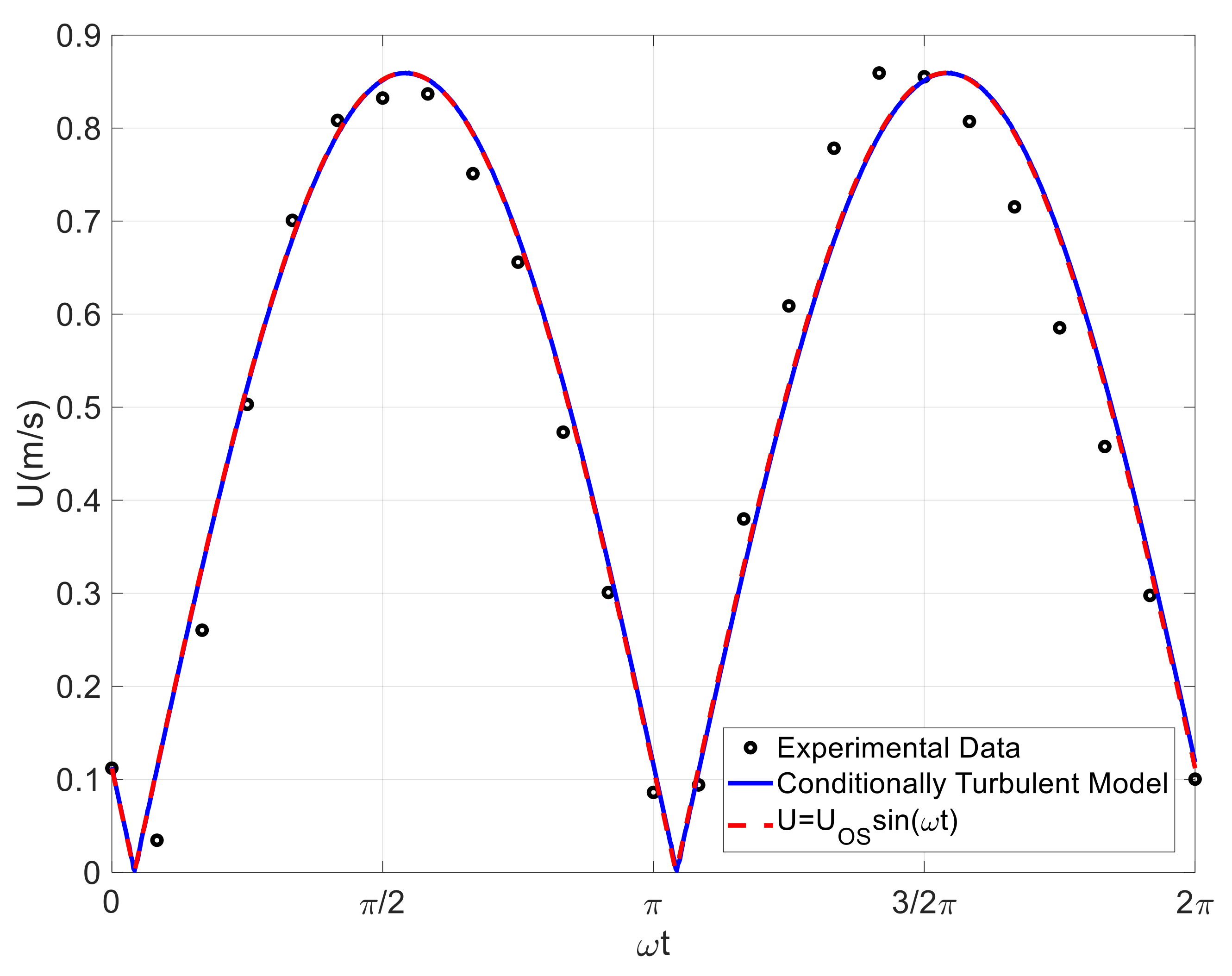
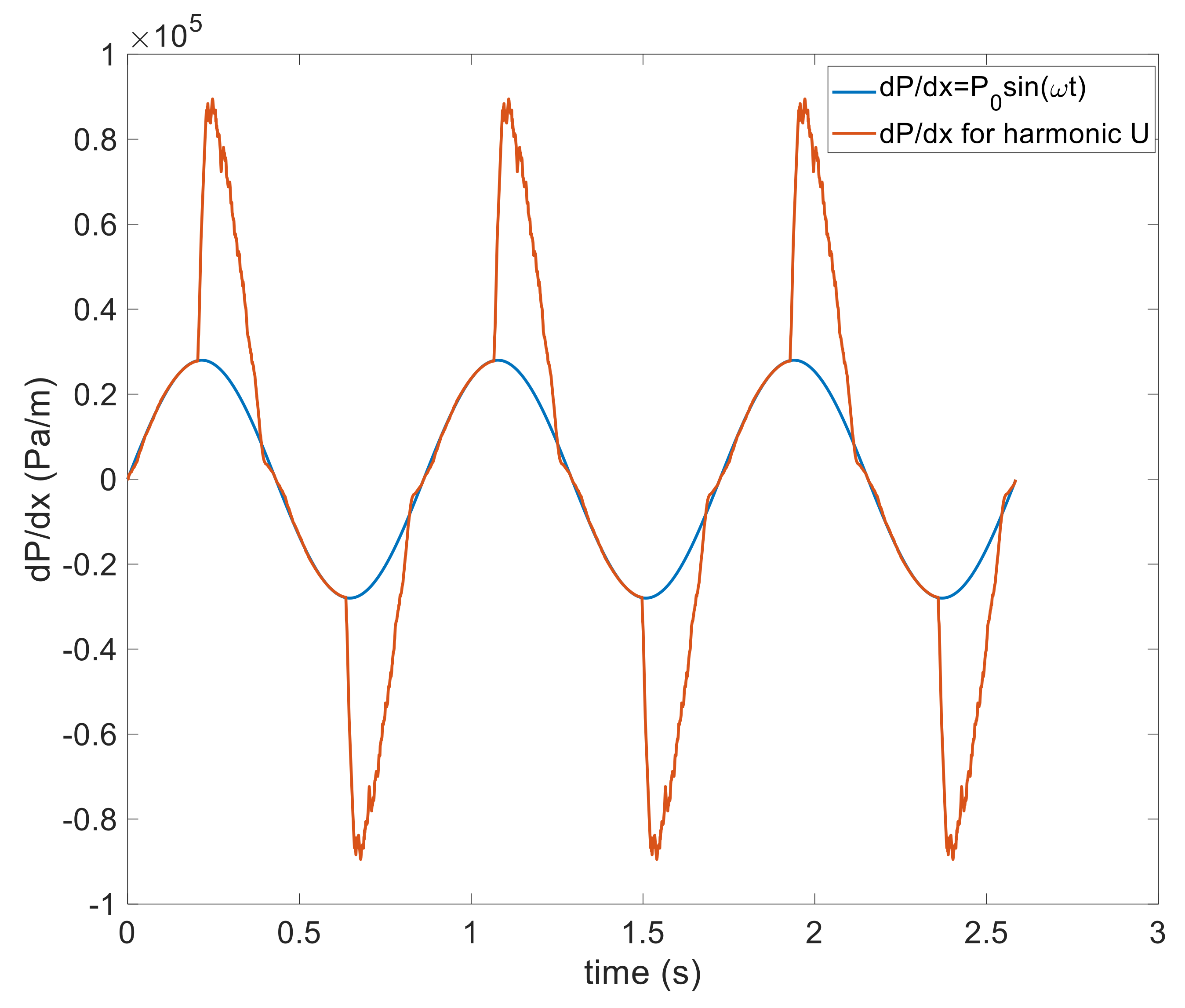
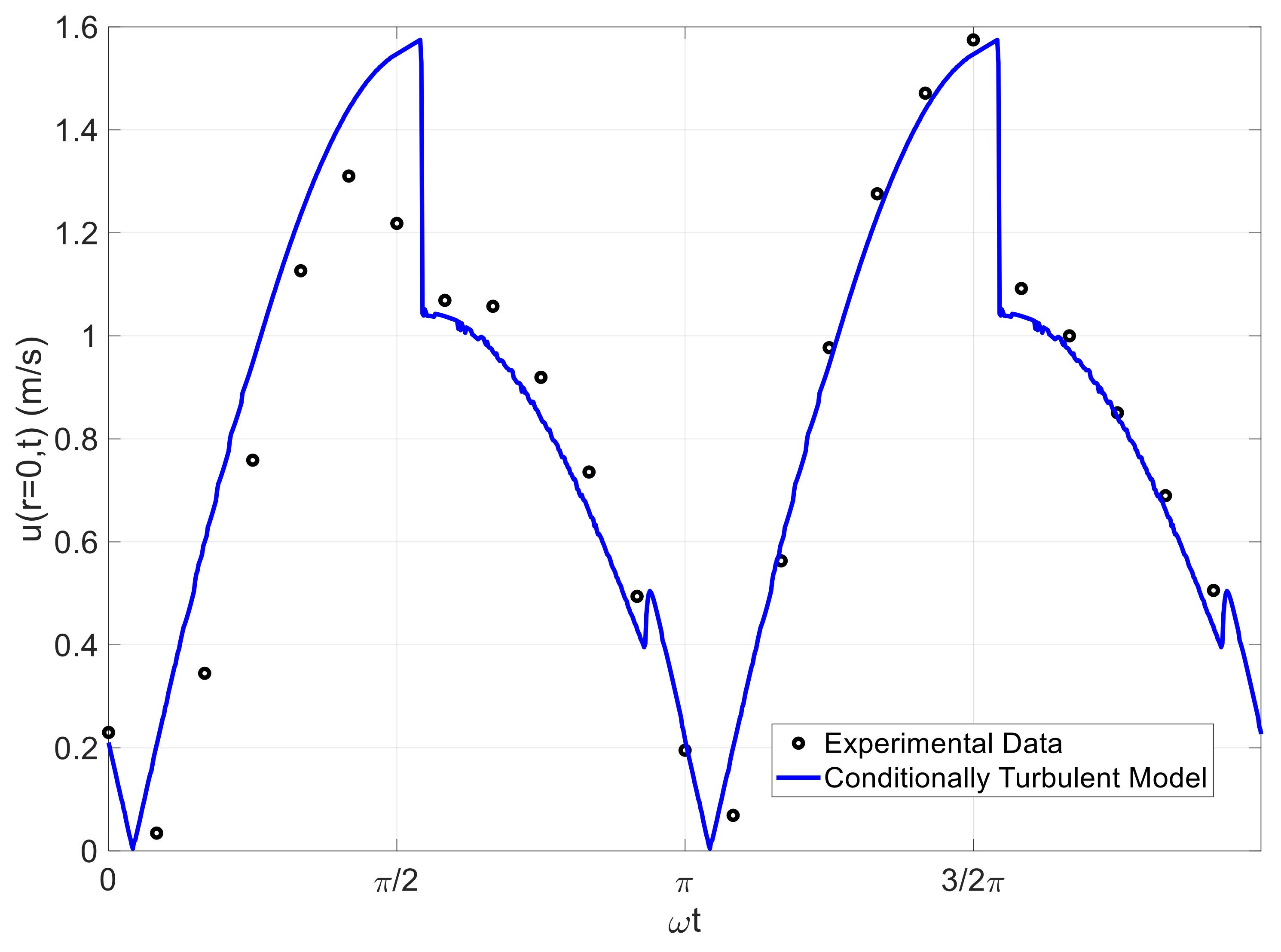
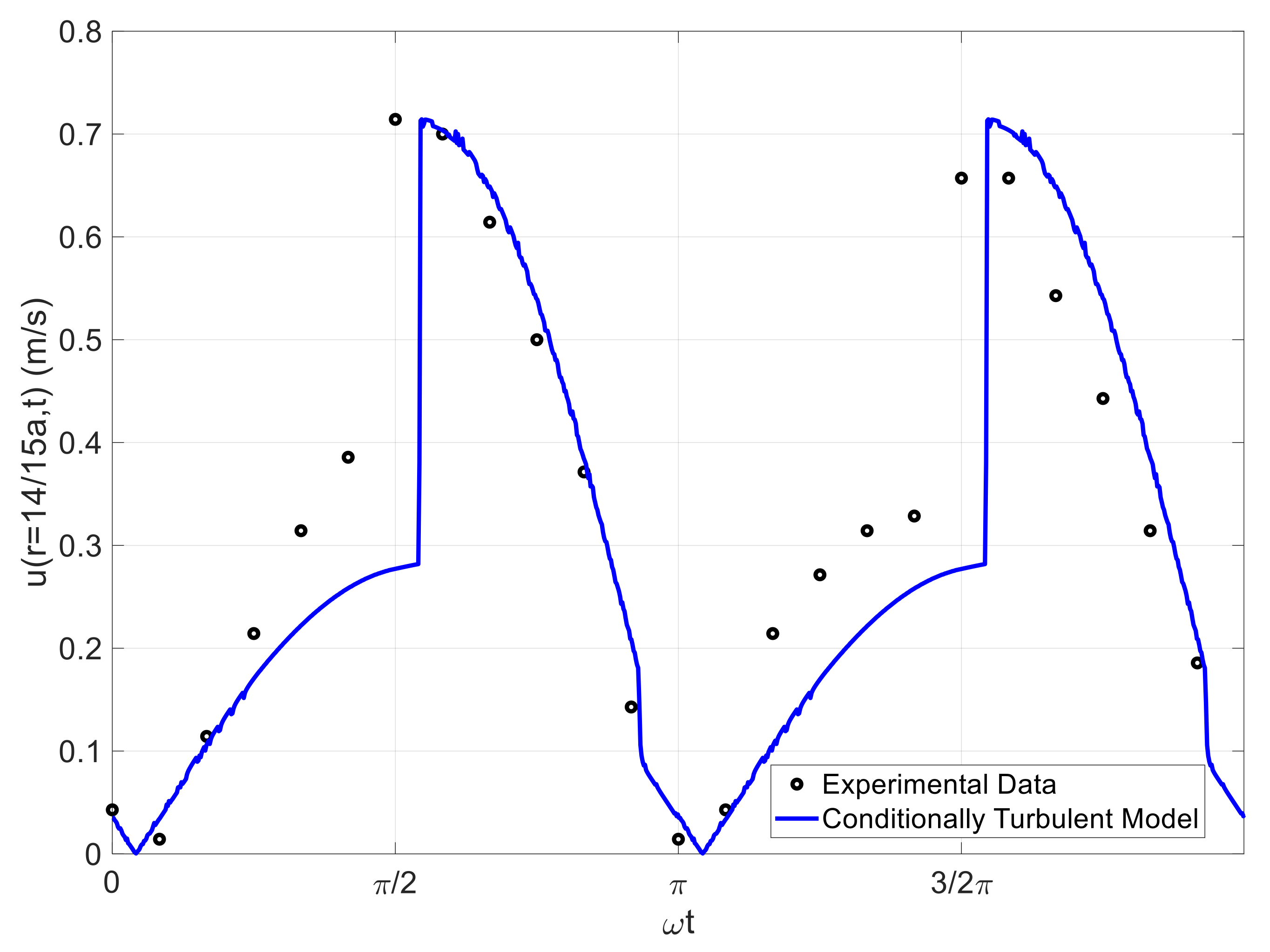
Figure 4, Figure 5, Figure 6 and Figure 7 show comparisons between the data and the numerical calculations for case 1 [5]: Figure 4 shows a comparison between the phase-averaged (bulk) velocity variations; Figure 5 shows the imposed pressure gradient; Figure 6 and Figure 7 show velocity comparisons at the pipe center-line and near-wall, respectively. As noted in Section 1, this experiment shows both critically and conditionally turbulent regimes within the same experiment. To achieve a harmonic variation of the bulk velocity computationally, the pressure gradient was adjusted iteratively, at each timestep, as described in Section 2.4; the differences between the bulk velocity rectified harmonic wave (Figure 4) never exceed 0.05%.
Computationally, the phase variation of the pressure gradient clearly shows the dramatic effect of modeled transition and relaminarization (see Figure 5). The sharp pressure rise and drop are clearly associated with the initiation and termination of the mixing-length term. As expected, these changes in pressure gradient are comparable to estimates based on steady laminar pipe-flow theoretical results and turbulent flow pipe-flow correlations [33].
It is evident, however, that the experiment does not produce a purely harmonic average flow oscillation (Figure 4). This could have been anticipated because the cam-and-piston arrangement used in the experiment does not produce purely harmonic motion. In particular, note that the second half of the cycle exhibits a phase shift consistent with a larger acceleration. This can be easily shown theoretically by analyzing the motion of a cam-and-piston arrangement. Nevertheless, the variations between data and computation were considered to be sufficiently close in order to facilitate comparison.
We now consider the velocity at the pipe centerline in Figure 6. As noted above, the experimental data show a clear asymmetry in which critically and conditionally turbulent regimes are present under nominally identical conditions. In the second half of the cycle, the flow is conditionally turbulent, i.e., it undergoes a transition to turbulence when d U / d t 0 as shown in Hino et al. [5]. However, in the first half of the cycle, the transition is clearly observed prior to the occurrence of the condition d U / d t = 0 . Even though this may be attributed to an inherent asymmetry in the pipe setup, this is probably not the case here. This is most likely due to the larger acceleration in the second part of the cycle due to the asymmetry of the cam-and-piston arrangement and can clearly be seen in Figure 4. Hence, we can conclude that this data set lies on, or very close to, the transition between critically and conditionally turbulent flow regimes.
Despite these small differences, the simple heuristic model shows rather good correspondence with the data. In the second half of the cycle (conditionally turbulent regime), the dramatic drop in the centerline velocity produced by initiating the mixing-length model is physically realistic and consistent with the “violent turbulent fluctuations” observed by Hino et al. [5]. However, due to the relatively large phase-differences between successive data points, it is not clear how accurately the instantaneous transition model captures the flow physics. It is evident from the first half of the cycle that the conditionally turbulent modeling assumption does not accurately model the transition process. Nevertheless, during both halves of the cycle, the turbulent flow development following transition is well predicted. As the flow becomes subcritical during the deceleration phases, and the mixing-length term is terminated, the computed centerline velocity shows a sharp velocity increase followed by a decrease. This is most probably non-physical behavior because relaminarization does not occur “violently“ as in the case of transition [5]. An improved model should include a sub-critical Reynolds number decay-type model, similar to that associated with steady flows undergoing relaminarization (Narasimha and Sreenivasan [6]). However, a steady/unsteady flow analogy cannot directly be used here because, in steady flows, observations are based on the Reynolds number being reduced and then remaining constant downstream [6]. This is where the analogy breaks down because the flow is not continuously varying downstream in analogy with a flow continuously varying in time. There are presently no empirical data known to the authors that would serve as a basis for such a model. In this context, large eddy simulations (LES) or DNS studies [19,20] could be very useful for developing such a model.
Figure 7 shows the corresponding data in the region close to the wall, at r/a = 14/15. Here, the prediction of a sharp increase in the near-wall velocity associated with transition, which is required to preserve conservation of mass, is qualitatively correct. As with the centerline velocity, however, it is not evident how accurately the timescales of transition are captured. The comparison with data in the acceleration phases of both half-cycles clearly shows the model deficiency in the laminar parts of the cycle. The significant under-prediction of the data is clear evidence that this flow is not purely laminar and contains some remnant turbulence generated earlier [5]. Note furthermore that the predictions in the initial part of the first acceleration phase are superior to those in the initial part of the second one. This may be due to differences in relaminarization following the different transition mechanisms, namely, critical and conditional.
An obvious weakness of the present model is the assumption of abrupt relaminarization during flow decelerations. Unfortunately, there is very little empirical data upon which to base even a simple heuristic model and this is an interesting opportunity for future experimental programs and simulation studies. One might consider an analogy between steady spatially and temporally decelerating flows [34,35], but this is not straightforward. For example, relaminarization occurs in “steady” pipe flows in which the Reynolds number becomes subcritical due to a gradually increasing pipe diameter (Narasimha and Sreenivasan [6]). In these flows, the skin friction attains its laminar value well upstream of the flow in the middle of the pipe. The location of the decaying peak turbulent kinetic energy y max moves toward the center of the pipe in proportion to the square root of the downstream distance. However, these observations are based on flows in which the Reynolds number is maintained constant, and hence there is no direct way to relate these to unsteady flows where the Reynolds number is continuously changing. Notwithstanding the deficiency in the prediction of abrupt relaminarization, this simple approach was deemed sufficiently accurate for preliminary design calculations.
Direct numerical simulation (DNS) studies, such as those conducted by Feldmann and Wagner [19,20], are of particular relevance from this point of view. They considered the oscillatory pipe flow case, Reos = 11,460 and α = 13 , which lies close to the transition criterion, namely, k = 882 versus 750 (Çarpınlıoğlu and Özahi [7]; also see Figure 1). An important difference between this DNS study and experimental investigations is that a harmonic pressure gradient and a harmonic average flow are imposed in the former and latter cases, respectively. This makes very little difference to the cross-sectional phase-averaged velocity in fully turbulent flows but can be significant in transitional flows, as shown in the example considered in Figure 4, Figure 5, Figure 6 and Figure 7. Despite these differences, sample DNS axial velocity traces and experimental observations across the pipe radius are qualitatively similar. For example, turbulence is generated during the decelerating phases while it decays during the acceleration phases. Furthermore, similar to experiments, the computations show considerable variability and asymmetry (cf. Hino et al. [23]). For example, turbulence generation can occur prior to, close to, or subsequent to the mean flow maxima. Phase-averaged results based on DNS can be an excellent vehicle for validating and calibrating simplified models.

3.2. Comparisons to Phase-Averaged Data

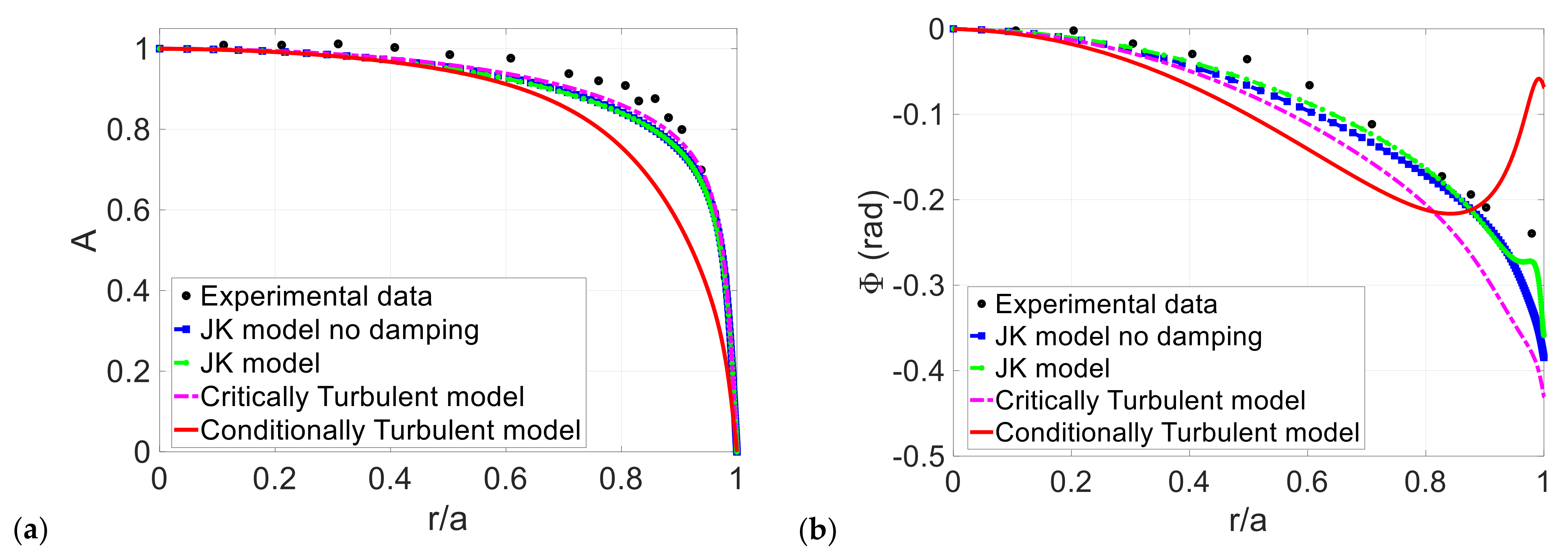
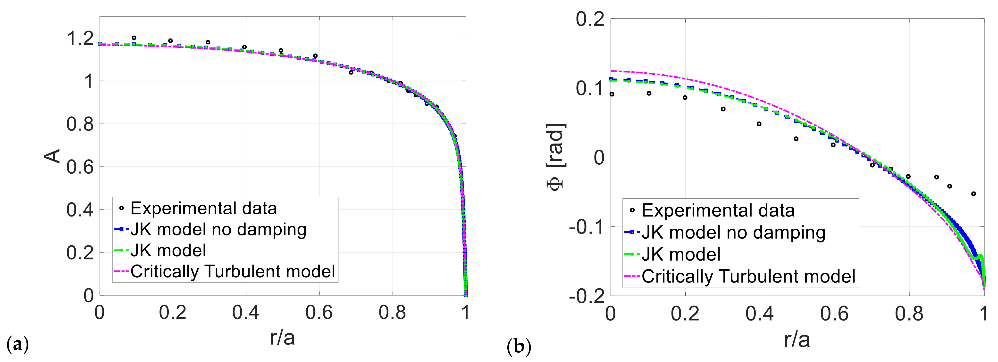
When data are presented in a phase-averaged manner, it is difficult to discern the mechanisms of transition and relaminarization, and indeed if they occur at all. Figure 8 presents the experimental data of Ohmi et al. [9] (Case 2: Reos = 19,300, α = 16.5 , see Table 1) with computational results of the various models including the Johnson–King (JK) model, with and without variable near-wall damping and critically and conditionally turbulent models. Note that this Reynolds number, the second-highest considered (see Table 1), is approximately 10 times larger than the accepted steady pipe flow value (~2000). Comparisons are shown for velocity amplitude ratio (Figure 8a) and phase shift (Figure 8b) as a function of the normalized pipe radius. For fully turbulent modeling, the flow is assumed to remain fully turbulent despite the fact that for part of the cycle the Reynolds number is subcritical. The physical justification of such a model is that the turbulence generated when the flow is supercritical does not decay sufficiently in the subcritical regime to warrant a transition or relaminarization model. For a flow oscillating in a quasi-steady manner, this would clearly not be the case. However, as the frequency is increased, such a scenario can be envisaged.
A clear observation here is that the conditionally turbulent model, i.e., where instantaneous transition and subsequent relaminarization are assumed, deviates significantly from the experimental data. This is true for both amplitude and phase comparisons. Based on previous arguments, this result is surprising because R e o s / α = 1170 in this case versus 2160 in Case 1, shown in Figure 4, Figure 5, Figure 6 and Figure 7. Indeed, it should be expected that this flow would exhibit a more laminar nature, but the comparison does not bear this out. It also appears that the flow is not critically turbulent because the deviations in phase are larger. Based on the two different damping forms presented here, it is speculated that this flow is essentially turbulent with perhaps some small relaminarizing effect near the wall. Hence, the R e o s / α scaling applicable to transition flows is not valid for flows that have a significantly higher R e o s .
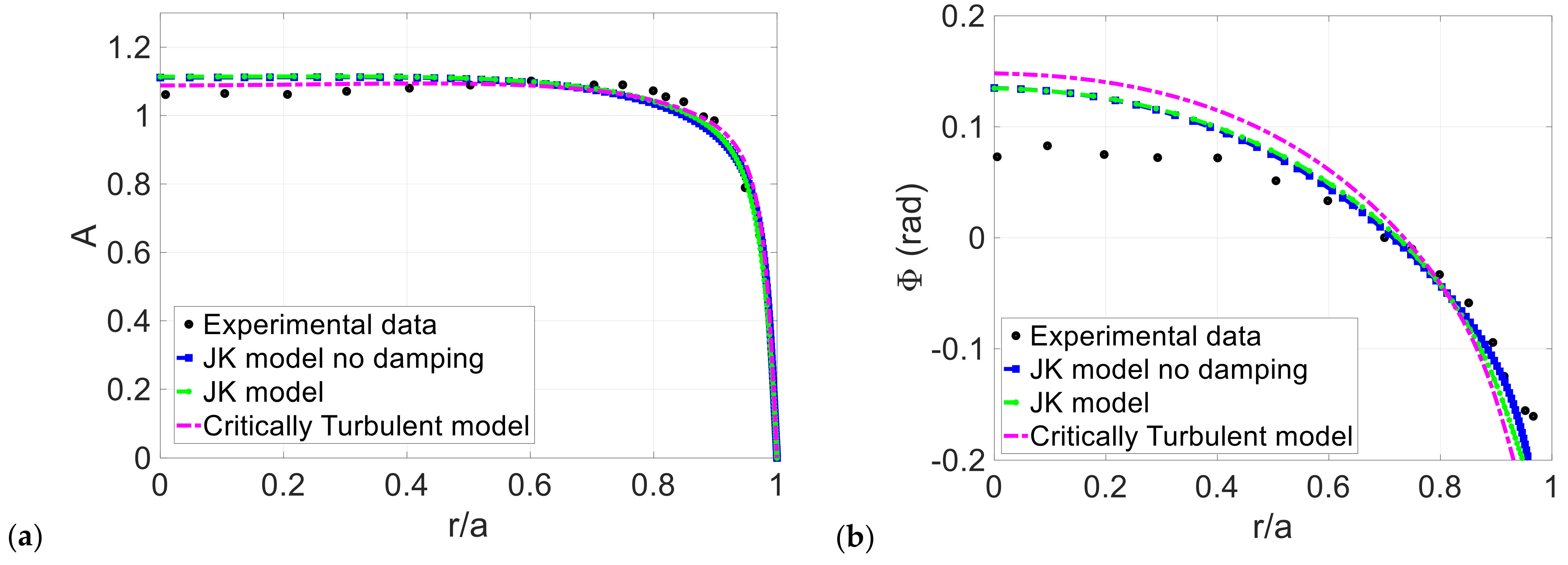
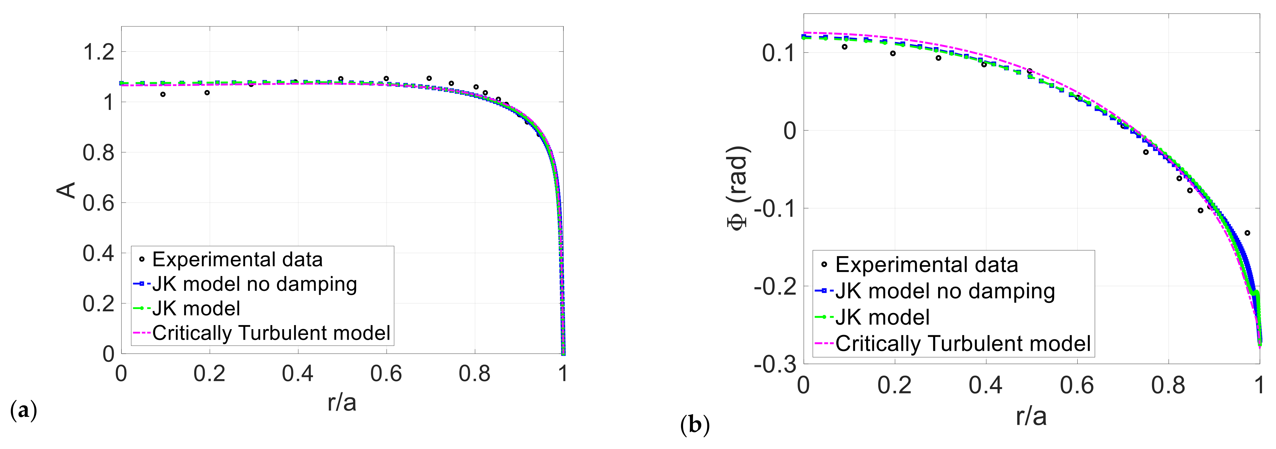
The subsequent Cases 3–5 are shown for amplitude and phase shift in Figure 9, Figure 10 and Figure 11 on the same basis as those shown in Figure 8. In Figure 9, the critically turbulent model produces slightly superior amplitude predictions but inferior phase predictions as in Figure 8, although these differences are very small. Furthermore, the results for all of the remaining cases suggest that unsteady effects are very small. The differences between computed and experimental amplitude are in general small and the differences in phase never exceed about 0.05 radians (3 degrees). This is probably within the experimental uncertainty, and hence no single model is considered significantly superior to any other. In light of this result, it is not surprising that the comparisons of cases 4 and 5 show rather good correspondence with the fully turbulent result because the R e o s / α values are substantially higher than cases 2 and 3. The introduction of the wall damping term has a very small effect and, in general, produces a small phase improvement accompanied by a slightly inferior amplitude prediction compared to the model with no damping. One limitation of the experimental data, probably due to practical difficulties, is that measurements very near to the wall were not made; hence, the model predictions could not be fully evaluated. Accurate modeling of the flow near the wall is vital for heat transfer predictions and should be considered in future experiments. Comparing phase-averaged turbulent velocity (u(r,t)) and turbulent stress ( u v ) profiles throughout a cycle (not shown) indicated that the inclusion of variable near-wall damping makes very little difference, with only a slightly increased overshoot.
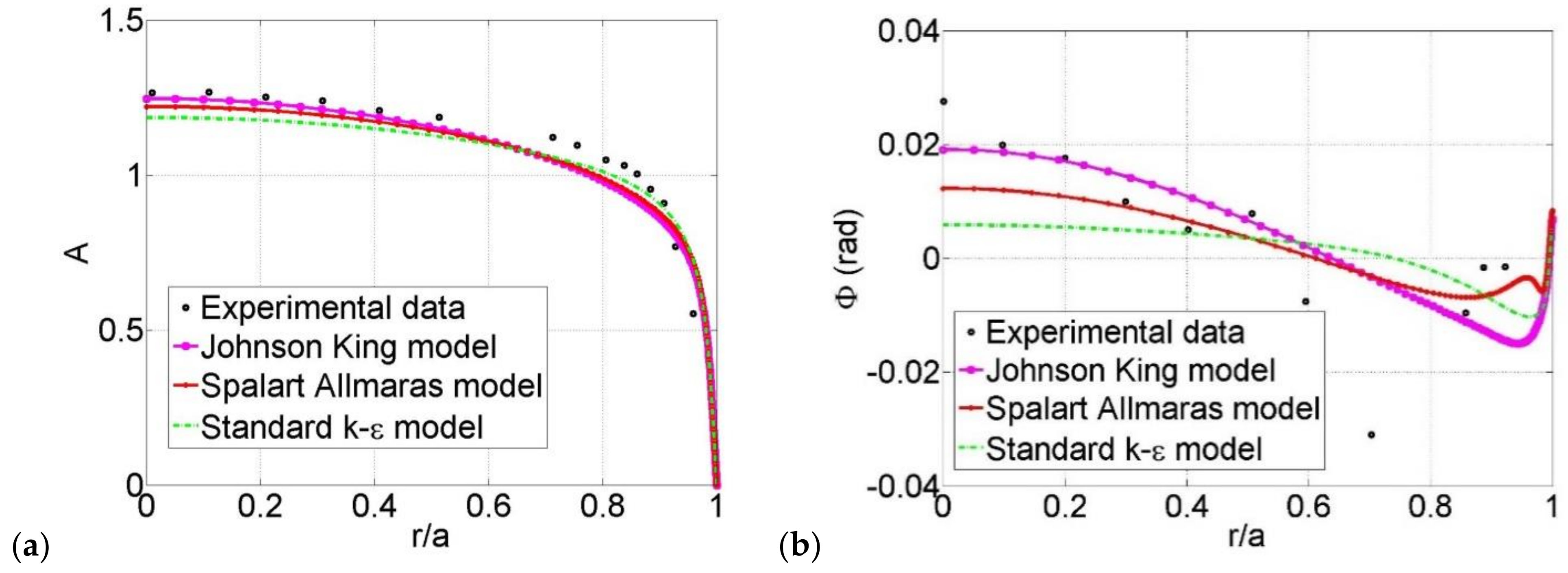
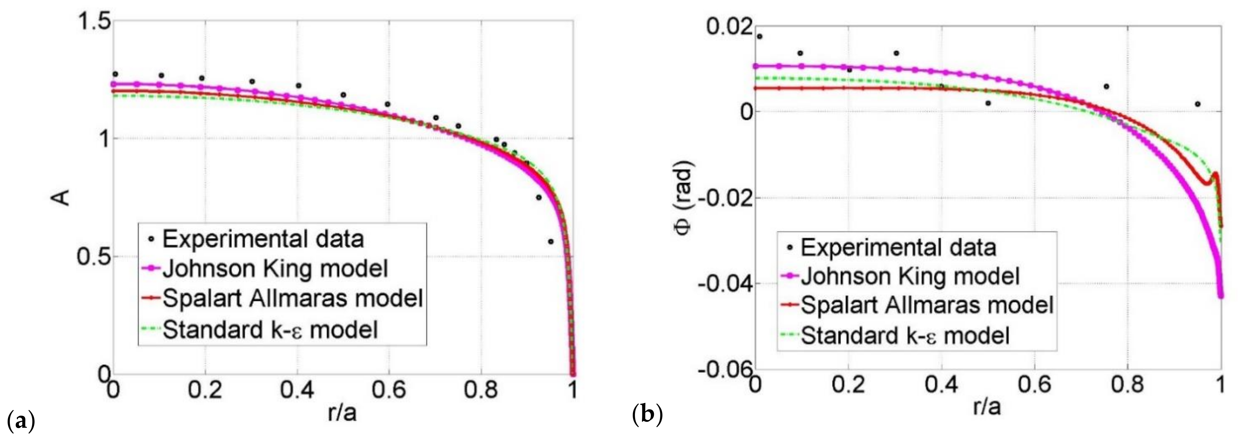
It was observed further that the results presented here were superior to the results of a standard kε turbulence model, particularly with regard to phase shift [17]. This may have been due to the fact that the standard kε model does not include a wall modification or a near-wall pressure gradient correction. Although the relatively simple Johnson–King model provided excellent correspondence with experimental data, popular and commonly used Spalart–Allmaras and k–ε turbulence models were assessed by means of the commercial software package Fluent, as described in Section 2.5. Cases 6 (Reos = 20,600, α = 7.9) and 7 (Reos = 40,600, α = 7.9) were selected for comparison.
For all computations, the oscillating pressure gradient was imposed by setting the pressure at one end as an oscillating function of time and at the second end as constant. Furthermore, 500 timesteps per cycle were employed and, as before, the solution was considered to be converged when the relative change in average velocity at each phase during successive cycles was less than 10−4 (see Section 2.3) A comparison between the JK and higher-order models implemented in Fluent for cases 6 and 7 is shown in Figure 12 and Figure 13. It can be seen that all of the models, including the JK model, yielded comparable and reasonable correspondence with the data. Nevertheless, it should be noted that phase-shifts are very small and these data do not represent a fully meaningful validation of the models. As mentioned above, future experiments at Womersley numbers at two orders of magnitude larger should be considered, consistent with large industrial machines [1]. It can be expected that the algebraic equilibrium JK model is computationally more efficient than either the Spalart–Allmaras or k–ε models because the latter require simultaneous solution one or two transport equations, respectively. A comparison of these results with simple mixing-length models, namely, those of Cebeci–Keller, Spalding–Patankar, and Crawford–Kays for cases 1–5 resulted in similar, but slightly inferior, results (not shown).

3.3. The Turbulent Womersley Number

Apart from the near-wall region, it is curious that the turbulent flow is mainly unaffected by the oscillations and shows relatively small amplitude and phase effects. One plausible explanation is that α is an inappropriate scaling parameter for turbulent flows; indeed, it was developed for laminar and transitional flows and represents the ratio of the pipe radius to the unsteady Stokes layer [36,37]. However, in a turbulent flow, the laminar kinematic viscosity should be replaced by a representative value near the wall. To remain consistent with the assumptions of the Johnson–King model, we take this to be the eddy viscosity at the peak turbulent kinetic energy ν t , max such that a turbulent, or effective, Womersley number is expressed as follows:
α t a ω / ν t , max
Using the definition
ν t , max = [ l 2 u / y ] max l m , max 2 τ w / ρ ν
we can write a “turbulent Womersley number” in the form
α t a ω / ν R e t = α R e t
where R e t u τ l m , max / ν , and l m , max corresponds to the distance from the wall at which the turbulent kinetic energy is a maximum. On the basis of steady turbulent pipe flow, we can estimate R e t > 10 1 , and hence we should expect α t to be at least 10 times smaller than its laminar counterpart. This provides a basic and rudimentary explanation of why deviations from a turbulent flow profile with small phase shifts are observed in the data sets considered here.
A similar scaling was proposed by Spalart and Baldwin [22], who argued that the outer layer of an oscillatory boundary layer (similar to a pipe flow), scales with u τ / ω . Using their definition, a turbulent Womersley number based on the friction velocity can be defined in the present context as
α t α R e τ
where R e τ = u τ a / ν . Note that the only difference between these two arguments is the use of the length-scale l m , max in the present case versus the use of a in the outer-layer model of Spalart and Baldwin [22].

4. Conclusions

Oscillatory pipe flows are particularly challenging to model because their flow state depends on both the Reynolds number and the dimensionless frequency or Womersley number. This paper presented a computational method that solves the one-dimensional Reynolds-averaged pipe-flow equation using a modified Crank–Nicolson method for oscillatory transitional and turbulent pipe flows. It included models for critically and conditionally turbulent flows and was validated against a wide range of existing experimental data. The equilibrium form of the Johnson–King model was implemented with the near-wall Mao–Hanratty modification to account for temporal changes in the pressure gradient. The critical Reynolds number was assumed to vary with the Womersley number, as observed in previous investigations, and transition and relaminarization were assumed to occur instantaneously. In the former case, this assumption was essentially valid, but in the latter case, substantial deviations between data and predictions were observed. An empirical relaminarization model, based on an analogy between steady spatial and unsteady temporal flow development was proposed but not implemented.
In the flows in which the oscillatory Reynolds numbers were at least 10 times higher than the commonly accepted steady critical value (~2000), fully or continuously turbulent models produced the best correspondence with experimental data. These models were considered sufficiently accurate for preliminary design calculations. Indeed, critical and conditionally turbulent models produced slightly inferior predictions and no significant benefit was observed when near-wall pressure gradient effects were implemented or when computationally expensive higher-order models were implemented. Nevertheless, the lack of data very close to the wall, and the resulting inability to conduct a detailed validation somewhat limited definitive conclusions. Given the experimental difficulties associated with near-wall measurements, namely, blockage due to hot-wire probes and reflections associated with optical methods, DNS can play an important role in elucidating near-wall physics and the development of models. Despite relatively large values of R e o s / α the unsteady effects in the turbulent flows considered here were relatively small. This was explained by considering that the turbulent viscosity is significantly higher than its laminar counterpart. Thus, the effective, or turbulent, Womersley number was significantly smaller than its laminar counterpart.
A great deal of research needs to be carried out in oscillatory turbulent pipe flows, particularly with regard to understanding and modeling relaminarization. Extensive opportunities exist for LES and DNS, in addition to an increase in the experimental database. Fundamental studies lack detailed turbulence statistics, near-wall, and wall shear stress measurements. Furthermore, many industrial applications demand accurate predictions of heat transfer at Reos > 106 and significantly higher α . A central challenge in achieving significantly higher α is that a factor-of-two increase requires a factor-of-four increase in frequency.

Author Contributions

Conceptualization, G.G.; methodology, D.G.; software, A.S.; validation, A.S.; writing—original draft preparation, D.G.; writing—review and editing, D.G.; supervision, D.G. and G.G; All authors have read and agreed to the published version of the manuscript.

Funding

This research received no external funding.

Institutional Review Board Statement

Not applicable.

Informed Consent Statement

Not applicable.

Data Availability Statement

All data and computation results are available upon reasonable request.

Conflicts of Interest

The authors declare no conflict of interest.

Nomenclature

A(r)velocity cross-sectional amplitude ratio
A+van Driest damping parameter
apipe radius
Dnear-wall damping term, 1 exp ( y u τ / ν A + )
dpipe diameter
kconstant in relation between Reos and α.
Lpipe length
lmturbulent mixing length
Ppressure
Ppressure difference
P0amplitude of the oscillating pressure gradient Δ P ( t ) / L = P 0 cos ω t
p+non-dimensional pressure gradient ( ν / ρ u τ 3 ) ( d P / d x )
p eff + normalized pressure gradient, defined in Equation (14)
Q(t)Time-dependent bulk volumetric flowrate
Reospeak oscillatory Reynolds number U o s 2 a / ν
rradial coordinate
ttime
t+ non-dimensional time t u τ 2 / ν
U ( t ) phase-averaged bulk velocity
Uosphase-averaged bulk velocity amplitude
u(r,t)local phase-averaged axial velocity
uoslocal phase-averaged velocity amplitude
uτfriction velocity τ w / ρ
u+non-dimensional velocity u / u τ
u v phase-averaged Reynolds stress
xaxial coordinate
ydistance from the wall y = a r
y+dimensionless distance from the wall y u τ / ν
αWomersley number a ω / ν
βouter-layer empirical constant, 0.08
λ Stokes parameter a ω / 2 ν
Φvelocity cross-sectional phase-shift relative to U ( t )
κvon Kármán constant, 0.4
ρfluid density
νkinematic viscosity
νtturbulent kinematic viscosity
τwwall shear stress
ωcircular oscillation frequency

References

  1. Radebaugh, R. Pulse tube cryocoolers. In Low Temperature and Cryogenic Refrigeration; Springer: Dordrecht, The Netherlands, 2003; Volume 99, pp. 415–434. [Google Scholar]
  2. McMahon, H.O.; Gifford, W.E. A new low-temperature gas expansion cycle—Part I. Adv. Cryog. Eng. 1960, 5, 354–366. [Google Scholar]
  3. Chan, C.K.; Nguyen, T.; Colbert, R.; Raab, J.; Ross, R.G., Jr.; Johnson, D.L. IMAS Pulse tube cooler development and testing. Cryocoolers 1999, 10, 139–147. [Google Scholar]
  4. Wollan, J.J.; Swift, G.W.; Backhaus, S.; Gardner, D.L. Development of a thermoacoustic natural gas liquefier. In Proceedings of the Conference 2002 AIChE New Orleans Meeting, New Orleans, LA, USA, 11–14 May 2002. [Google Scholar]
  5. Hino, M.; Sawamoto, M.; Takasu, S. Experiments on transition to turbulence in an oscillatory pipe flow. J. Fluid Mech. 1976, 75, 193–207. [Google Scholar] [CrossRef]
  6. Narasimha, R.; Sreenivasan, K.R. Relaminarization of fluid flows. Adv. Appl. Mech. 1979, 19, 221–309. [Google Scholar]
  7. Çarpınlıoğlu, M.Ö.; Özahi, E. An updated portrait of transition to turbulence in laminar pipe flows with periodic time dependence (a correlation study). Flow Turbul. Combust. 2012, 89, 691–711. [Google Scholar] [CrossRef]
  8. Sergeev, S.I. Fluid oscillations in pipes at moderate Reynolds numbers. Fluid Dyn. 1966, 1, 121–122. [Google Scholar] [CrossRef]
  9. Ohmi, M.; Iguchi, M.; Kakehashi, K.; Masuda, T. Transition to turbulence and velocity distributions in an oscillating pipe flow. Bull. JSME 1982, 25, 365–371. [Google Scholar] [CrossRef] [Green Version]
  10. Ohmi, M.; Iguchi, M. Critical Reynolds number in an oscillating pipe flow. Bull. JSME 1982, 25, 165–172. [Google Scholar] [CrossRef]
  11. Eckmann, D.M.; Grotberg, J.B. Experiments on transition to turbulence in oscillatory pipe flow. J. Fluid Mech. 1991, 222, 329–350. [Google Scholar] [CrossRef]
  12. Akhavan, R.; Kamm, R.D.; Shapiro, A.H. An investigation of transition to turbulence in bounded oscillatory Stokes flows—Part 1: Experiments. J. Fluid Mech. 1991, 225, 395–422. [Google Scholar] [CrossRef]
  13. Das, D.; Arakeri, J.H. Transition of unsteady velocity profiles with reverse flow. J. Fluid Mech. 1998, 374, 251–283. [Google Scholar] [CrossRef] [Green Version]
  14. Merkli, P.; Thomann, H. Transition to turbulence in oscillating pipe flow. J. Fluid Mech. 1975, 68, 567–575. [Google Scholar] [CrossRef]
  15. Zhao, T.S.; Cheng, P. Experimental studies of the onset of turbulence and frictional losses in an oscillatory pipe flow. Heat Fluid Flow 1996, 17, 356–362. [Google Scholar] [CrossRef]
  16. Lodahl, C.R.; Sumer, B.M.; Fredsøe, J. Turbulent combined oscillatory flow and current in a pipe. J. Fluid Mech. 1998, 373, 313–348. [Google Scholar] [CrossRef]
  17. Ahn, K.H.; Ibrahim, M.B. Laminar/turbulent oscillating flow in circular pipes. Int. J. Heat Fluid Flow 1992, 13, 340–346. [Google Scholar] [CrossRef] [Green Version]
  18. Walther, C.; Kuhl, H.-D.; Schulz, S. Numerical investigation on the heat transfer in turbulent oscillating pipe flow. Heat Mass Transf. 2000, 36, 135–141. [Google Scholar] [CrossRef]
  19. Feldmann, D.; Wagner, C. Direct numerical simulation of fully developed turbulent and oscillatory pipe flows at Reτ = 1440. J. Turbul. 2012, 13, 1–28. [Google Scholar] [CrossRef]
  20. Feldmann, D.; Wagner, C. On phase asymmetries in oscillatory pipe flow. In New Results in Numerical and Experimental Fluid Mechanics X; Dillmann, A., Heller, G., Krämer, E., Wagner, C., Breitsamter, C., Eds.; Notes on Numerical Fluid Mechanics and Multidisciplinary Design 132; Springer: Cham, Switzerland, 2018; pp. 113–122. [Google Scholar]
  21. Hanjalić, K.; Jakirlić, S.; Hadžić, I. Computation of oscillating turbulent flows at transitional re-numbers. In Turbulent Shear Flows 9; Springer: Berlin, Heidelberg, 1995; pp. 323–342. [Google Scholar]
  22. Spalart, P.R.; Baldwin, B.S. Direct simulation of a turbulent oscillating boundary layer. In Turbulent Shear Flows 6, Proceedings of the Selected Papers from the Sixth International Symposium on Turbulent Shear Flows, Université Paul Sabatier, Toulouse, France, 7–9 September 1987; Andre, J.-C., Cousteix, J., Durst, F., Launder, B.E., Schmidt, F.W., Whitelaw, J.H., Eds.; Springer: Berlin, Germany, 1989. [Google Scholar]
  23. Hino, M.; Kashiwayanagi, M.; Nakayama, A.; Hara, T. Experiments on the turbulence statistics and the structure of a reciprocating oscillatory flow. J. Fluid Mech. 1983, 131, 363–399. [Google Scholar] [CrossRef]
  24. Sumer, B.M.; Jensen, B.L.; Fredsøe, J. Turbulence in oscillatory boundary layers. In Advances in Turbulence; Comte-Bellot, G., Mathieu, J., Eds.; Springer: Berlin/Heidelberg, Germany, 1987; pp. 556–567. [Google Scholar]
  25. Ghodke, C.; Apte, S. DNS study of particle-bed-turbulence interactions in an oscillatory wall-bounded flow. J. Fluid Mech. 2016, 792, 232–251. [Google Scholar] [CrossRef]
  26. Ghodke, C.D.; Apte, S.V. Roughness effects on the second-order turbulence statistics in oscillatory flows. Comput. Fluids 2018, 162, 160–170. [Google Scholar] [CrossRef]
  27. Greenblatt, D. Hybrid turbulence model for unsteady boundary layers. AIAA J. 1998, 36, 481–484. [Google Scholar] [CrossRef]
  28. Johnson, D.; King, L. A mathematically simple turbulence closure model for attached and separated turbulence boundary layers. AIAA J. 1985, 23, 1684–1692. [Google Scholar] [CrossRef]
  29. Mao, Z.X.; Hanratty, T.J. Studies of the wall shear stress in a turbulent pulsating pipe flow. J. Fluid Mech. 1986, 170, 545–564. [Google Scholar] [CrossRef] [Green Version]
  30. Spalart, P.R.; Allmaras, S.R. A one-equation turbulence model for aerodynamic flows. In Proceedings of the 30th Aerospace Sciences Meeting and Exhibit, Reno, NV, USA, 6–9 January 1992. [Google Scholar]
  31. Sexl, T. Über den von E. G. Richardson entdeckten Annulareffekt. Z. Physik 1930, 61, 349–362. [Google Scholar]
  32. Duan, Z.; Yovanovich, M.M.; Muzychka, Y.S. Pressure drop for fully developed turbulent flow in circular and non-circular ducts. J. Fluid Eng. 2012, 134, 6. [Google Scholar] [CrossRef]
  33. Schlichting, H. Boundary Layer Theory; McGraw-Hill: New York, NY, USA, 1979. [Google Scholar]
  34. Greenblatt, D.; Moss, E.A. Rapid temporal acceleration of a turbulent pipe flow. J. Fluid Mech. 2004, 514, 65–75. [Google Scholar] [CrossRef]
  35. Greenblatt, D.; Moss, E.A. Pipe-flow relaminarization by temporal acceleration. Phys. Fluids 1999, 11, 3478–3481. [Google Scholar] [CrossRef]
  36. Akhavan, R.; Kamm, R.D.; Shapiro, A.H. An investigation of transition to turbulence in bounded oscillatory Stokes flows—Part 2: Numerical simulations. J. Fluid Mech. 1991, 225, 423–444. [Google Scholar] [CrossRef]
  37. Womersley, J.R. Method for the calculation of velocity, rate of flow and viscous drag in arteries when the pressure gradient is known. J. Physiol. 1955, 127, 553–563. [Google Scholar] [CrossRef] [PubMed]
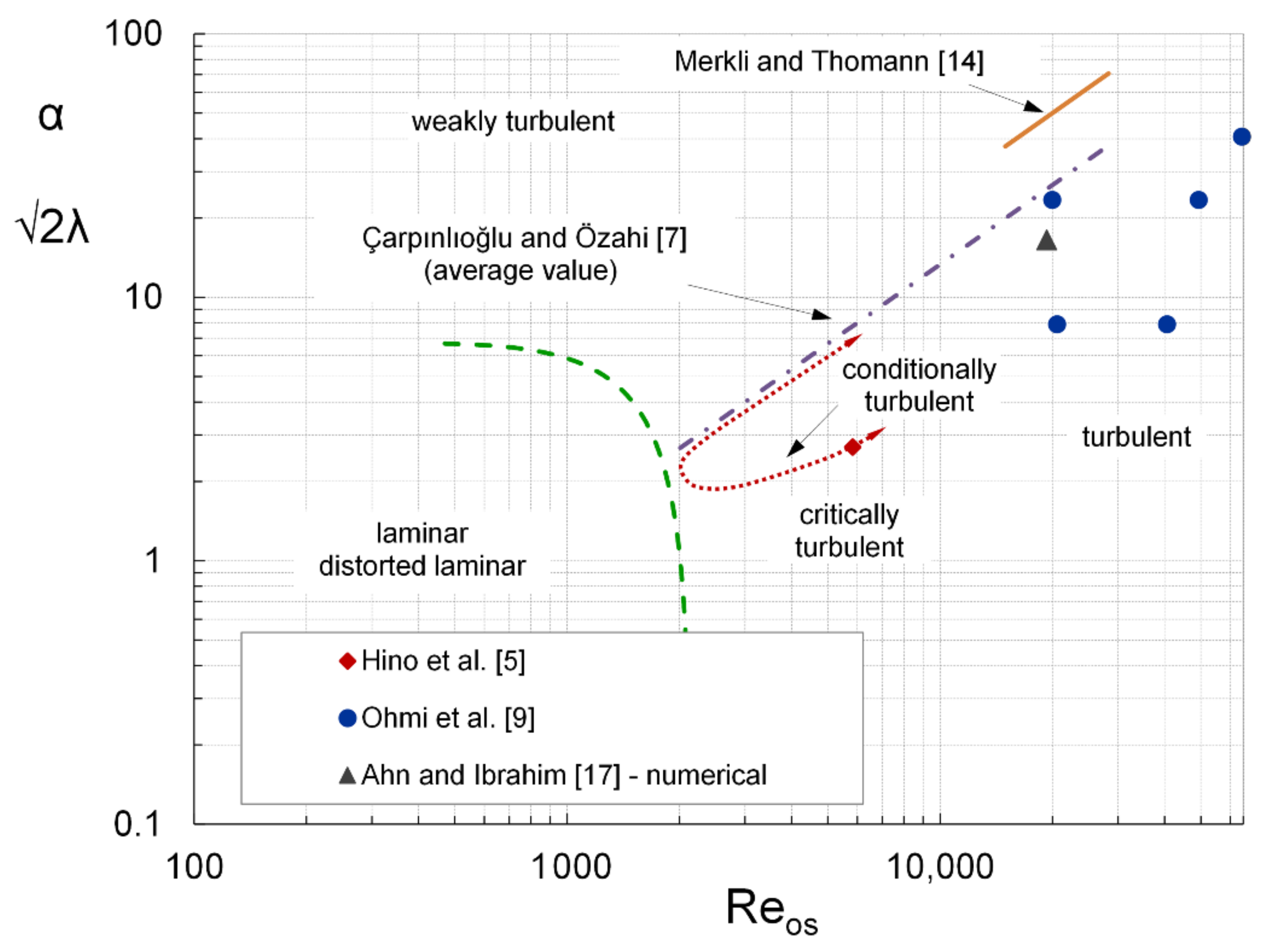
Figure 1. Characteristic diagram indicating the onset of transition and the resulting different flow regimes. k = 750 based on the extensive review by Çarpınlıoğlu and Özahi [7] and k = 400 according to Merkli and Thomann [14]. Data used for comparison to computational results (Hino et al. [5], Ohmi et al. [9], and Ahn and Ibrahim [17]) are indicated by symbols.
Energies 14 01410 g001
Figure 2. Schematic of the pipe-flow problem with coordinates and variables defined.
Energies 14 01410 g002
Figure 3. Amplitude and phase computations (see Equations (17) and (18)) compared to the analytical laminar solution [31,33] together with computation results corresponding to different turbulent flow regimes for increasing Reos at constant α = 10: (a) amplitude ratio; (b) phase-shift.
Energies 14 01410 g003
Figure 4. Comparison between the computationally enforced harmonic bulk flow and the phase-averaged experimental data for Case 1: Reos = 5830, α = 2.70.
Energies 14 01410 g004
Figure 5. Comparison between the pressure gradient before and after enforcing of harmonic average flow oscillations, corresponding to Case 1: Reos = 5830, α = 2.70.
Energies 14 01410 g005
Figure 6. Comparison between the conditionally turbulent model and the experimental data for phase-averaged velocity at the pipe centerline (r/a = 0) for Case 1: Reos = 5830, α = 2.70.
Energies 14 01410 g006
Figure 7. Comparison between the conditionally turbulent model and the experimental data for phase-averaged velocity near the wall (r/a = 14/15) for Case 1: Reos = 5830, α = 2.70.
Energies 14 01410 g007
Figure 8. Comparison between experimental data and various turbulence and transition models for Case 2: Reos = 19,300, α = 16.5: (a) amplitude ratio; (b) phase-shift.
Energies 14 01410 g008
Figure 9. Comparison between experimental data, turbulence models, and the critically turbulent assumption for Case 3: Reos = 20,000, α = 23.4 : (a) amplitude ratio; (b) phase-shift.
Energies 14 01410 g009
Figure 10. Comparison between experimental data, turbulence models and the critically turbulent assumption (Case 4: Reos = 49,400, α = 23.4): (a) amplitude ratio; (b) phase-shift.
Energies 14 01410 g010
Figure 11. Comparison between experimental data, turbulence models and the critically turbulent assumption (Case 5: Reos = 64,500, α = 40.5): (a) amplitude ratio; (b) phase-shift.
Energies 14 01410 g011
Figure 12. Comparison between the Johnson–King turbulence model and higher-order turbulence models (Case 6: Reos = 20,600, α = 7.9): (a) amplitude ratio; (b) phase-shift.
Energies 14 01410 g012
Figure 13. Comparison between the Johnson–King turbulence model and higher-order turbulence models (Case 7: Reos = 40,600, α = 7.9): (a) amplitude ratio; (b) phase-shift.
Energies 14 01410 g013
Table 1. Experimental data sets with corresponding experimental conditions that were used for validation of the computational results presented.
CaseReferenceReos α
1Hino et al. [5]58302.70
2Ahn and Ibrahim [17]19,30016.5
3Ohmi et al. [9]20,00023.4
4Ohmi et al. [9]49,40023.4
5Ohmi et al. [9]64,50040.7
6Ohmi et al. [9]20,6007.9
7Ohmi et al. [9]40,6007.9
Publisher’s Note: MDPI stays neutral with regard to jurisdictional claims in published maps and institutional affiliations.