1. Introduction
Power losses in transmission lines (cable lines, overhead wires) always occur depending on different physical phenomena. Among the power losses sources in the lines, the basic one is caused by the conductor heating while the current flows. The energy is released as Joules of heat [
1,
2]. The character and power of loads supplied by the transmission line in the design stage should avoid cable overloading. Mostly, there should be highlighted nonlinear loads which generate higher current harmonics to the supply network. These load types have a negative influence on the transmission line. Higher harmonics significantly impact the power losses and cause the cable conductor temperature to increase [
3,
4]. Assume that conductors work in these conditions for a long time. This may lead to insulation degradation and severe damage to the supplying cables. Supply equipment failure affects the economic losses in production enterprises due to unplanned demurrage and off-switching. It also generates additional costs linked with installation repairing. The costs and times of repair, especially for underground cable lines, are very high, so their occurrence should be minimized.
This article presents a simplified method for the calculation of active power losses and correlates it to the IEC-60287-1-1:2006 + A1:2014 standard method and the second one using the Bessel function. The obtained results may constitute a starting point to calculate the temperature distribution for different thermal backfills or determine the cable conductor’s optimal diameter and insulation.
The common element for all used methods [
5] concerning active power loss calculations in power cables determines the resultant resistance,
, for a given current harmonic order (h). In each method, both skin and proximity effects are considered. The first method is based on the Bessel function. It allows finding a solution to the equation in polar coordinate systems associated with wave propagation and spherical potentials. In calculations the conductor resistance variation caused by the skin effect is considered as a correction factor for resistance,
. The second method allows obtaining active power losses using the resultant surface resistance, considering the current penetration depth for uniform current flowing through a cross-section that is deep and wide. The next one is analytically described by the French researcher Levasseur based on skin effect observation and using frequency changes in the Kelvin effect calculations [
6]. The most popular active power loss calculation method is described in the IEC-60287-1-1:2006 + A1:2014 standard. This method uses factors correlating to the skin effect.
In the currently used methods [
5,
7], the increase in resistance for the fundamental frequency is considered no matter what the cable cross-section area is. In such small cross-sections (e.g., 25 mm
2), the depth of the current penetration—resulting from the skin effect—is greater than the radius of the low-voltage cable’s conductor. Hence, the conclusion is that the skin effect does not occur in this case and that the previously mentioned methods introduce an error in calculating the value of active power losses. However, in the authors’ new method the penetration depth factor concerning the radius of the considered cable conductor is considered.
It is difficult to carry out a laboratory experiment because of the relatively high RMS current values and current total harmonic distortion (THDI) needed for a wide range of low-voltage cable cross-section areas. Therefore, in this article power losses due to skin effect are used only for theoretical calculations for the comparison of different methods.
The main contribution of this work can be summarized as follows:
Presentation of a new active power loss calculation method based on the current penetration depth (CPD) factor depending on the analyzed current frequency.
Comparison of the new method to already-existing methods.
The active power loss increment for distorted currents is compared to the ideal 50 Hz sine wave for three calculation methods.
2. The Influence of Current Distortion on Power Cable Core Parameters
The current harmonic sources in the supply lines are nonlinear loads. Examples of nonlinear loads used by residential consumers are LED lights and power supplies for computers, TV sets, mobile and tablet chargers, and other electronic equipment. Thus, the universal usage of such loads is visible. They have an insignificant influence on the power network due to the low power of individual devices. However, the adverse impact increases if those devices work in bigger groups.
The opposite situation can be noticed for industrial consumers. Single loads have significant power (from several dozen kW to a few MW). In the power system infrastructure, the economy can be planned without considering important reserve factors for these loads. Such a situation can be acceptable for linear cases, because usually for this type of issue calculations are performed when planning the electrical systems. The current distortion level has a pivotal influence on the power cables’ real load value, supplying receivers for nonlinear loads. Among nonlinear high-power loads, we can highlight in particular power electronic converters such as rectifiers (full-bridge, six-pulse, twelve-pulse), frequency converters, and arc furnaces [
8,
9,
10].
The higher harmonics appearing in the current frequency spectrum for nonsinusoidal waveforms can be described as [
11,
12,
13]:
where:
is the DC component of the load current,
is the active current component,
is the reactive current component,
is the active current component of the higher harmonics,
is the reactive current component of the higher harmonics.
In relation to the standards [
14], the current harmonics are considered up to 40 order. The authors took into account these requirements and conducted a power loss analysis according to these guidelines (up to the 40th order).
Total harmonic distortion (THD) is a parameter describing the current deformation level and can be expressed by Equation (2):
where:
is the effective value of the signal of the fundamental component,
is the effective value of the signal of the n-th harmonic.
The significant participation of higher current harmonics can negatively affect the rest loads installed in the same power system due to the voltage deformation, further interaction, and increase in the current and voltage higher harmonic levels [
15,
16,
17,
18,
19].
Power cables are used widely in power systems, especially in industry. The cables must meet the following requirements:
- −
Electrical (current carrying capacity, short-circuit durability, high insulation resistance);
- −
Mechanical (special working conditions, environmental conditions, non-flammability, cable routing).
Due to this, the comprehensive requirements should be taken into account during the design process.
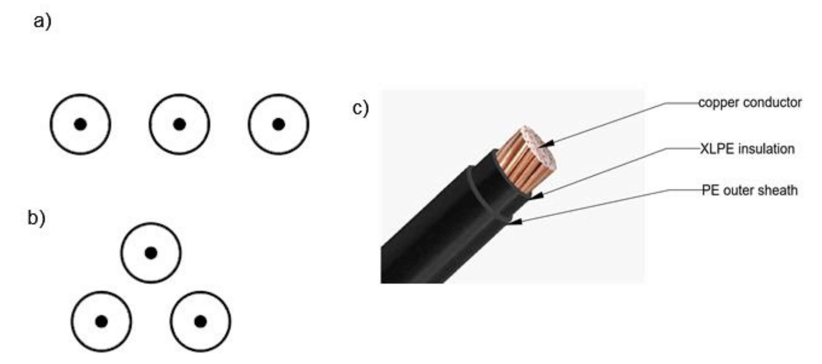
Figure 1 presents possible cable arrangement methods (flat or trefoil) for three single-core cables and cable construction.
The highest operating temperatures for different cable insulation types, according to PN-HD 60364-5-52:2011 [
20], are:
- −
polyvinyl chloride (PVC): 70 °C;
- −
cross-linked polyethylene (XLPE) and ethylene-propylene rubber: 90 °C.
Both construction and the used materials have a significant influence on cable heating. The cable core material determines the conductivity. The insulation material and its thickness impact the electric strength, mechanical durability, and cable heating (temperature distribution). An example of this is that cables with XLPE insulation increase the cable’s optimal operating temperature compared to PVC or PE insulation. Along with insulating properties, it exhibits chemical stability and is leak-proof.
Additionally, when the cable is equipped with a shield on each core in the case of multi-core cable or single-core cables, the sheath levels the proximity effect. The low-voltage cables that are mostly used are not shielded, so this effect cannot be neglected in these construction types. Increasing the accuracy of calculations can contribute to lowering the cost of building cable lines.
Cable routing and their backfill have non-negligible effects on the temperature distribution and maximal permissible load current. The most popular thermal backfills used in cables laid in the ground are dry sand, a sand-bentonite mixture (SCM), sand, and Portland cement (with a 12:1 ratio) [
21,
22,
23]. There are also advantages of new materials, such as geopolymers, which have better thermal conductivity properties and safer for the environment [
24]. Backfill’s higher thermal conductivity allows conducting the cable’s heat during current flow. The use of backfill also reduces the formation of dry zones around cables, which harm heat dissipation. When the cable temperature rises, the electric conductivity decreases due to the decrease in the electrons’ mobility in the metal conductor. Aluminum cables/wires are most often used in power systems, including AsXSn, steel-aluminum (AFL), and aluminum alloys AlMgSi (BLX-T). This directly affects the lower conductivity value compared to copper cores.
The two-dimensional temperature distribution in the steady state for cables in the thermal backfill can be calculated independently for a chosen cable routing according to [
25]:
where:
denotes the temperature at any point in the plane around the underground cable,
is the temperature-dependent thermal conductivity,
is the volumetric heat source per unit volume.
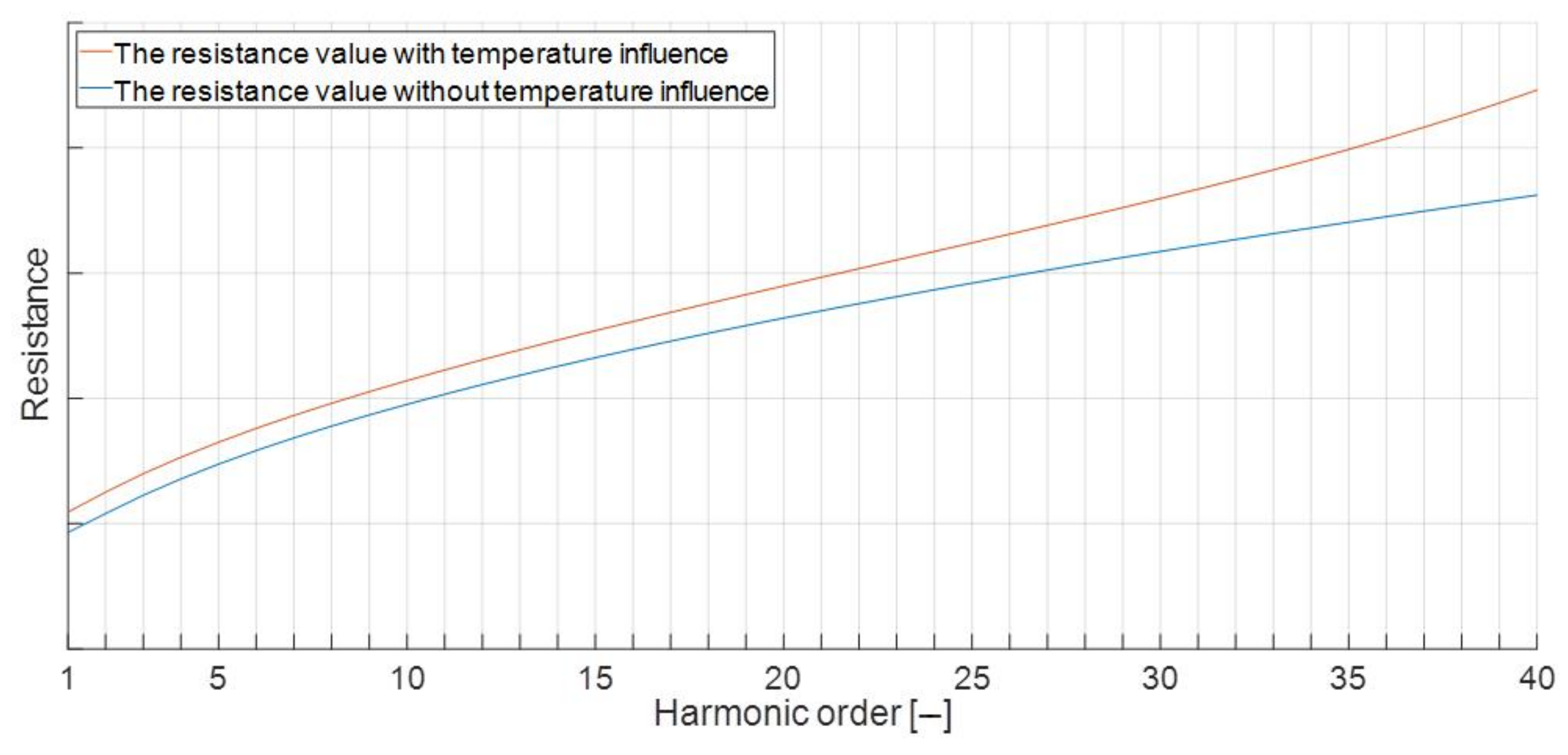
It should be noticed that the skin effect causes an irregular current intensity distribution in the cable conductor. The highest current density appears at the outer layer of the conductor cable. Therefore, a significant temperature increase occurs. The temperature changes inside the cable core, which can be calculated from Equation (3); intensifies the resistance increase; and, therefore, effects the equivalent resistance changes and power losses in nonlinear loads. This impact is illustrated in
Figure 2 [
7].
In this article, the temperature effect on the resistance value was skipped to highlight in particular the skin effect on the cable working conditions.
3. Active Power Losses
When the current is flowing through the conductor, power losses are generated as heat. This phenomenon was observed and described independently by Joule and Lenz in the 19th century and is known as Joule-Lenz heat.
The equation for the conductor heat losses is given by [
26]:
where:
is the conductor resistance, in ,
is the RMS current value in .
For nonsinusoidal current flow in the conductor, the power loss calculation is more complicated because it requires the consideration of the skin effect and the proximity effect [
5,
27,
28,
29]. The proximity effect can be neglected for a sufficiently large distance between each cable core or shielded cables. For a distorted current, the total active power losses in a cable are equal to the sum of each current harmonic power loss and can be expressed as:
where:
is the amplitude of the current fundamental harmonic,
is the percent value of the n-th harmonic.
The
resistance for any harmonic can be calculated based on the current penetration depth. According to this, we can calculate the resistance value for each current harmonic:
where:
is the wire length in ,
is the equivalent of cross-section area including the skin depth effect in .
In the case of a circular cross area, the effective area is described as:
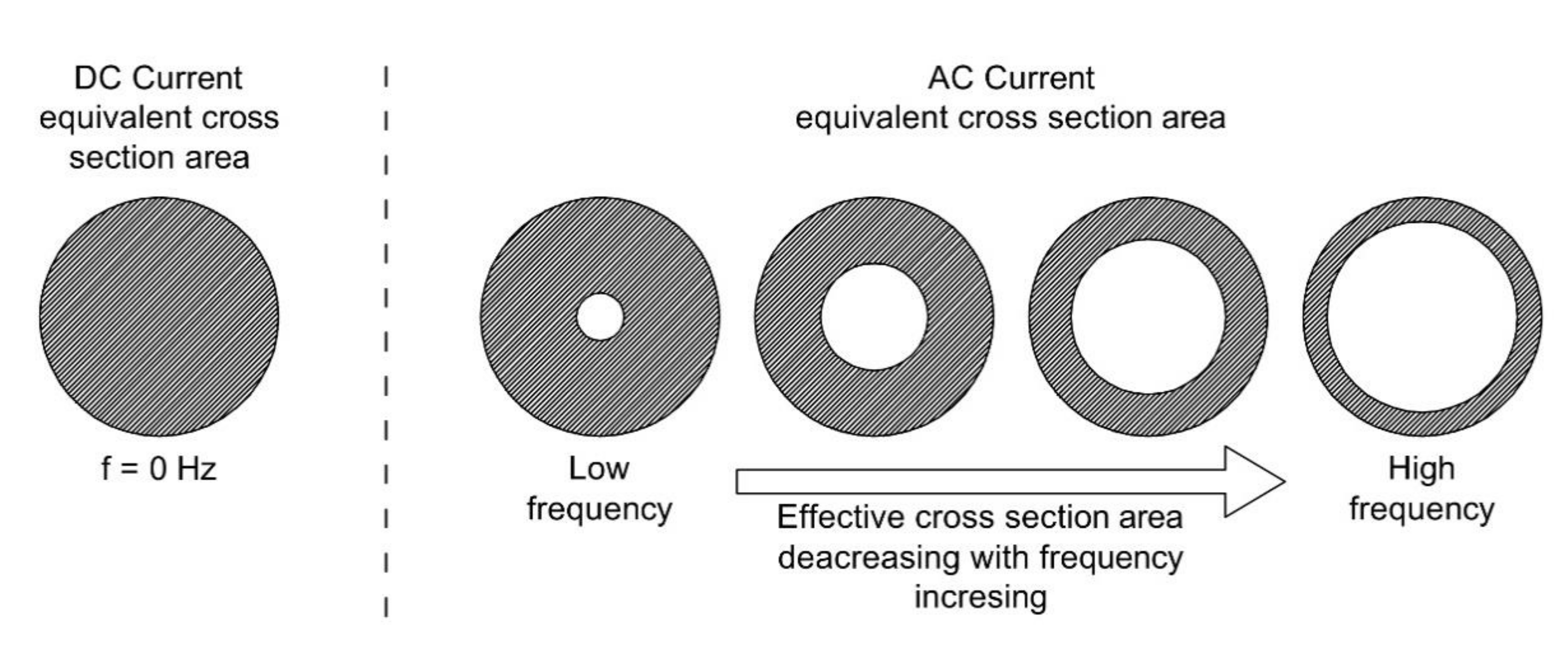
The current penetration depth (expressed by Equation (8)) describes how far (counting from the external edge) the current flows [
5]. In this way, it is easy to notice that the effective conductor cross-area through which a current of a given frequency flows is lower than the area resulting from the conductor’s geometric dimensions (
Figure 3):
where:
is the harmonic order number in ,
is the basic harmonic frequency in ,
is the vacuum permeability in ,
is the relative permeability in ,
is the conductivity of the material in .
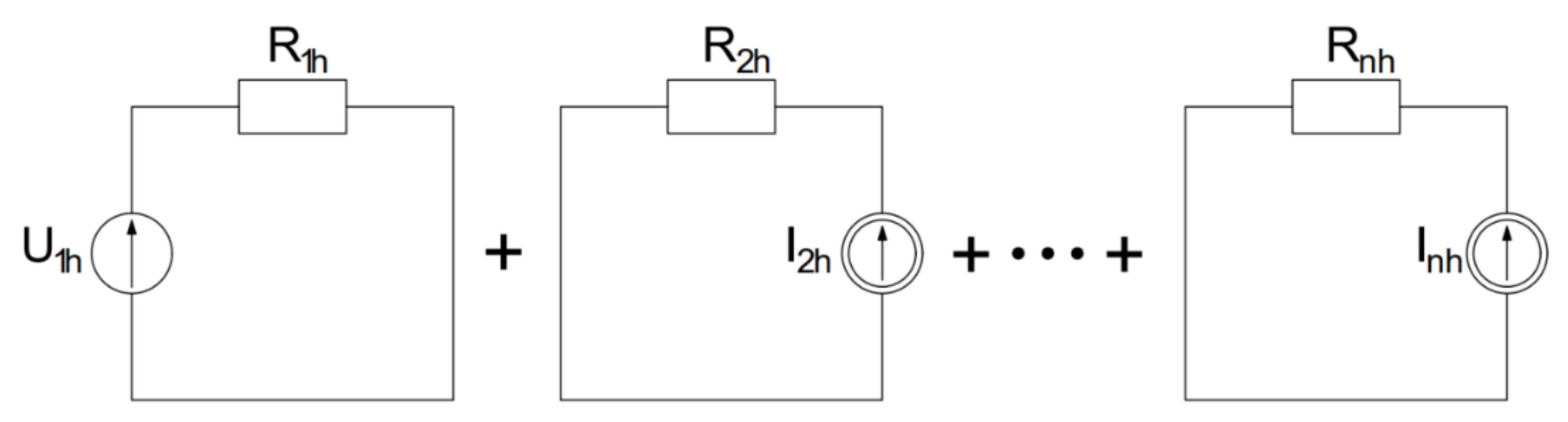
Resistance calculations were performed using the superposition method for a chosen current frequency (
Figure 4). This approach allows for each harmonic to determine the cable power losses by creating an equivalent circuit.
In turn, the IEC-60287-1-1:2006 + A1:2014 [
30] standard shows the calculation methodology for the resistance variations as a result of the skin effect as follows:
where:
is the AC resistance of the conductor in ,
is the DC resistance of the conductor in ,
is a skin effect factor in
is a proximity effect factor in
is the coefficient depending of the number of cable cores (for a single-core cable ) in .
The Bessel function were used as a third method [
31,
32,
33] according to the formulas:
where:
are Bessel functions of the first kind of the zeroth and first order, respectively.
The calculated resistance value as a frequency function is obtained as:
Active power loss calculations for cable cases were conducted for the three described methods, skipping the proximity effect ( value used in Equation (9) was equal to 0) to show only the influence of the skin effect.
4. Simulation Model
With the use of the Matlab software (MathWorks Inc., Natick, MA, USA), we developed a model allowing us to compare the three calculation methods generating the active power losses in the power cables considering the skin effect. The first model was completed using the IEC-60287-1-1:2006+A1:2014 [
30] standard guidelines, and the second one was completed using the Bessel function. Both methods’ results were compared to those of the third one, which was developed by the authors (the algorithm presents the method in
Figure 5).
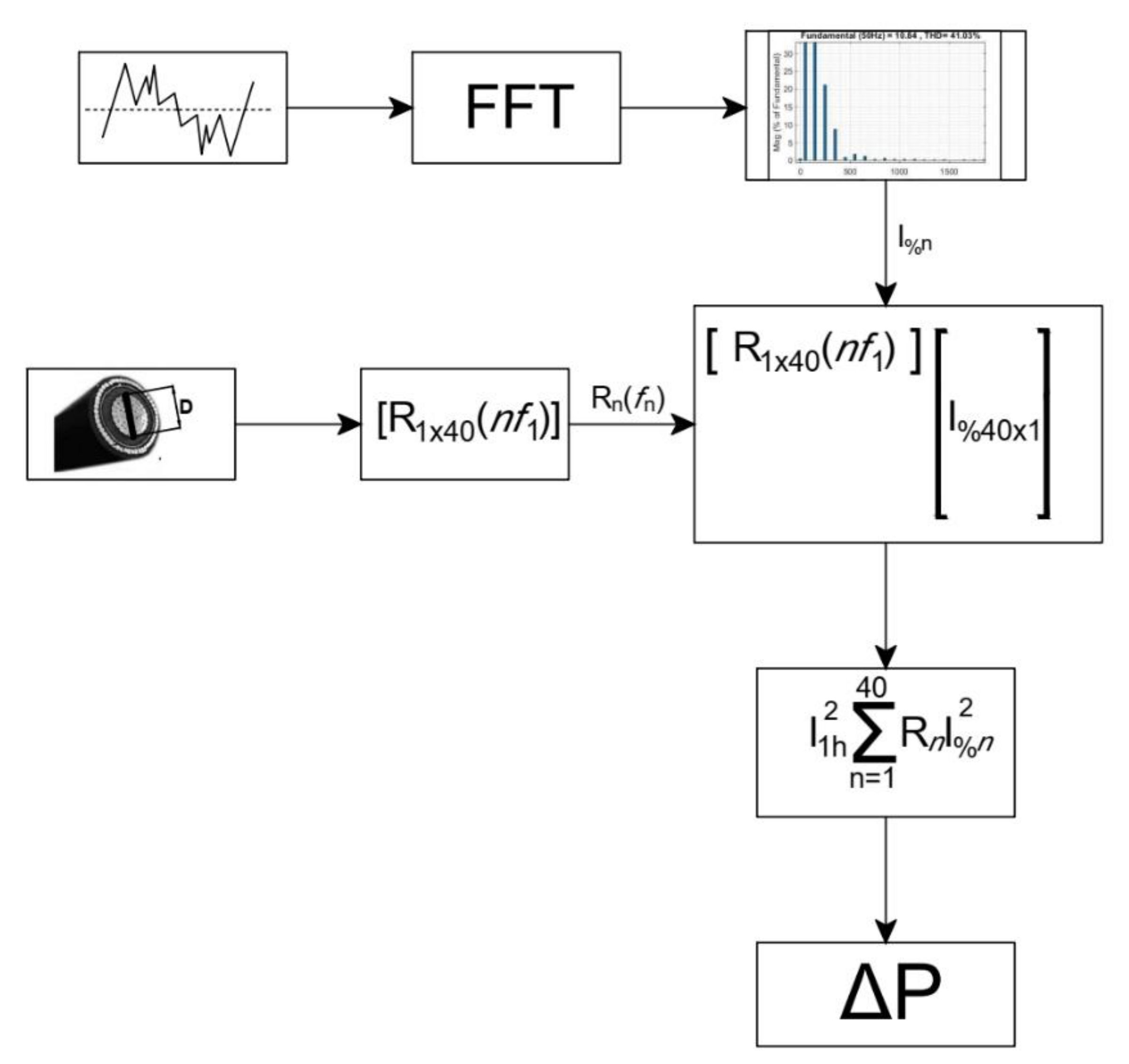
An algorithm illustrating the third one that was developed according to the authors’ proposition is presented in
Figure 5. This model was realized with the current penetration depth (CPD) method used for the given frequencies.
This is a description of the authors’ method:
Based on the measured distorted current waveform, we calculated the harmonic spectrum (using FFT analysis) to obtain the percentage magnitude values for each frequency (concerning the first harmonic order
For a given cable, the calculation conductor resistances suitable for the given harmonics (estimated based on Equations (6)–(8)) were based on the current penetration depth.
We multiplied the current I%n2 vector and the resistance vector.
We summarized the obtained values to achieve the total active power losses for the whole current harmonics spectrum (Equation (5)).
All the described methods were used to determine the power losses for three chosen nonsinusoidal currents:
- −
Distorted current waveform measured for bridge rectifier load in the real-life laboratory arrangement (),
- −
Measured waveform (from 1st point) with the added in-phase sinusoidal wave with a magnitude equal to half the basic harmonic of the distorted waveform (),
- −
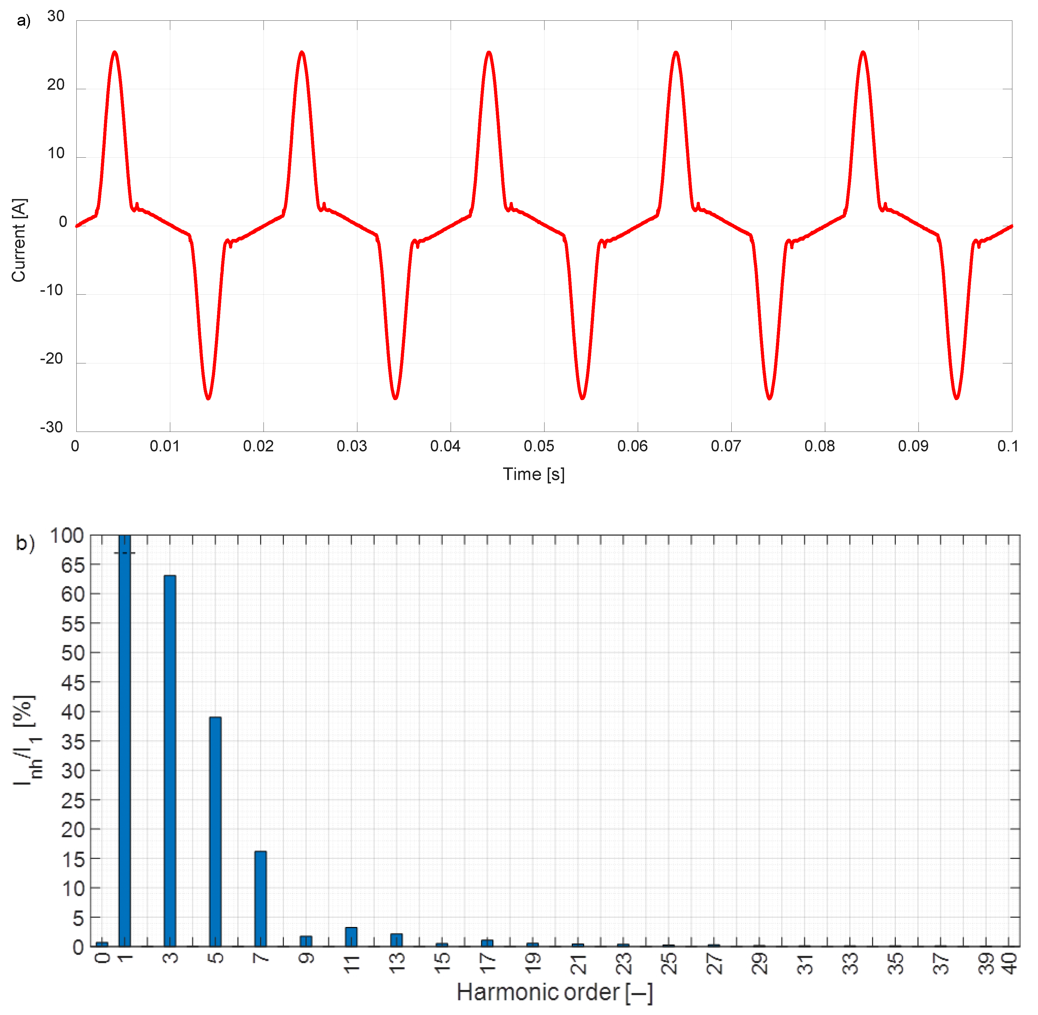
Measured waveform (from 1st point) with added shifted 90° sinusoidal wave with a magnitude equal to half the basic harmonic of the distorted waveform ().
An example waveform and its harmonic spectrum is shown in
Figure 6.
All the calculations were carried out for cables from
to
in a flat arrangement and the distances between each phase cable were equal to 2d (where d is the diameter). These calculations were conducted for the copper conductor and PVC insulation. For each cross-sectional area, the long-term current carrying capacity data were taken from the manufacturer’s catalogue. There were three calculation series for the current equal to
,
and
of the maximum current-carrying capacity for a unitary cable length equal to 1 m [
34].
5. Research Results
This chapter presents the numerical calculations of the power loss values generated in the power cables, taking into account the skin effect for the described methods. The first one is based on the IEC-60287-1-1:2006 + A1:2014 [
30] standard, the second is based on the Bessel function, and the third is illustrated by the algorithm proposed by the authors. The results calculated for the different power cables and current shapes are presented in
Table 1,
Table 2 and
Table 3.
The results were obtained for a unitary cable length equal to 1 m. For the longer line lengths, the active power losses are proportional to the length.
There is no effect of the current value on the voltage supply deformation in the presented methodology and, therefore, on the current deformation. Hence, for three loads the active power losses change with the current load square. For the active power losses calculation prepared for sinewave current, it is assumed that the current flows through the whole conductor cross-section. Therefore, the skin effect (for 50 Hz, the penetration depth is 9.6 mm) is not considered.
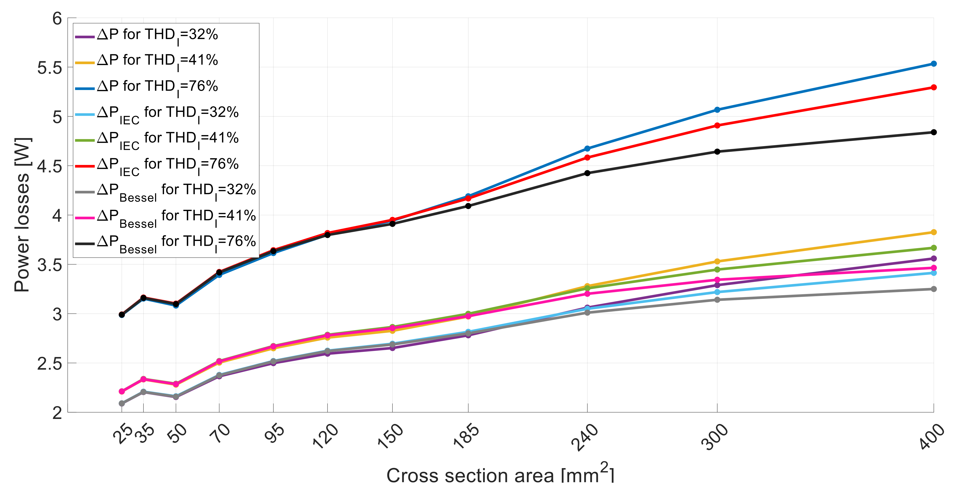
Additionally, the difference between each compared method is illustrated in
Figure 7 (the results received for
and
exhibit similar tendencies, therefore we illustrated only one case).
The differences between the analyzed methods are dependent on the cable cross-section area. For cables, the 25, 35, 50, 70 mm2 obtained results for the unitary power losses are very similar. The differences are maximally equal to 0.1 W—the skin effect is limited due to the small cable radius. If the CPD is smaller than the cable radius, the effective resistance for each harmonic increases. It is easier to understand power losses dependence for small cross-sections. The presented methods gave more divergent values for cross-sections higher than 185 mm2.
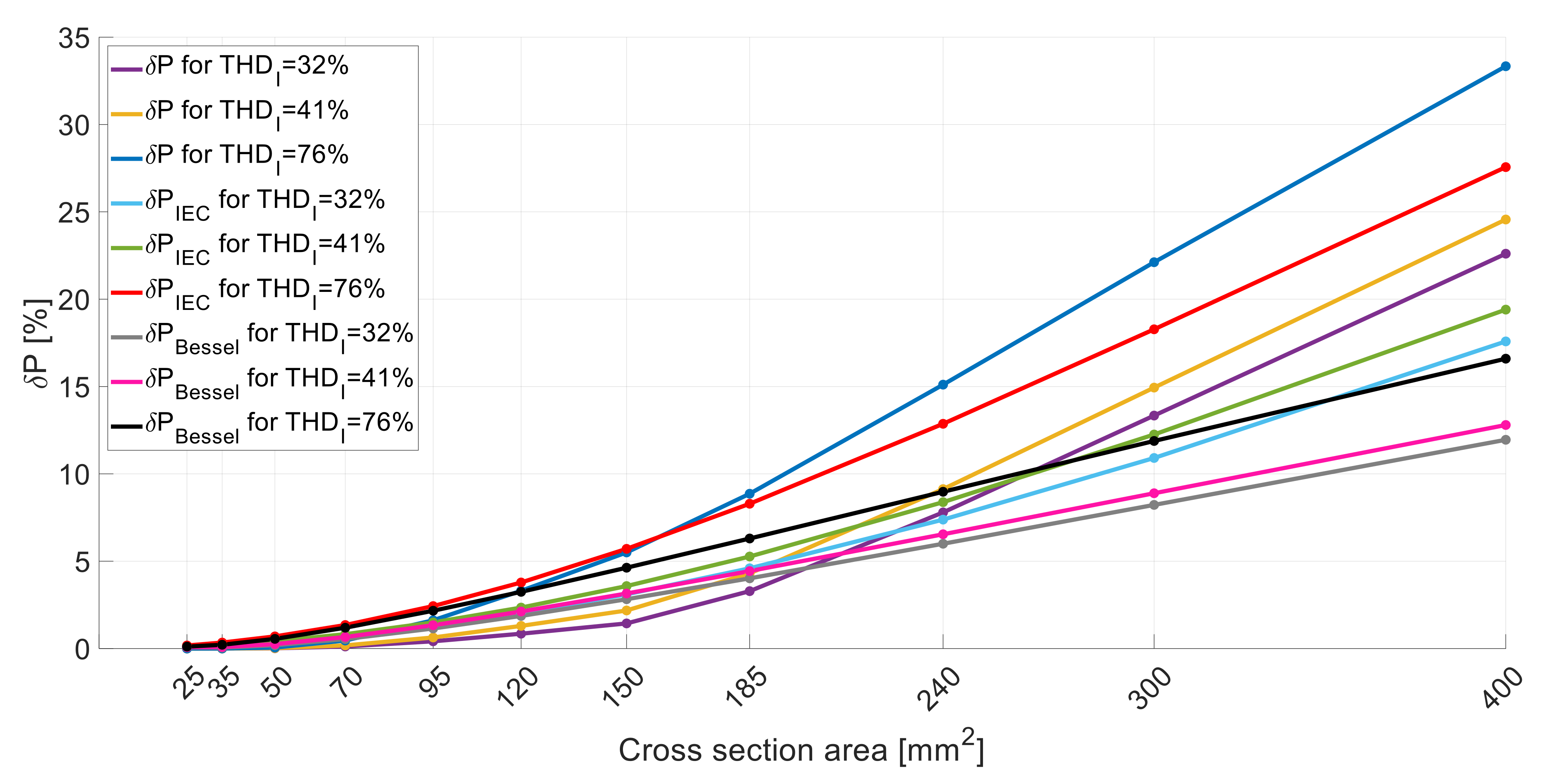
Figure 8 shows the percentage of active power losses calculated for distorted currents compared to the ideal sinusoidal wave for a 50 Hz frequency and the same RMS value. For small cable cross-sectional areas (lower than 50 mm
2), the relative active power loss growth is less than 1% for all the analyzed current distortion cases. For cross-section areas higher than 50 mm
2, the percentage of power loss rises. For a 400 mm
2 cable and a current THD equal to 76%, the highest increments (27.6% for the IEC method, 16.6% for the Bessel function method, and 33.3% for the method proposed by the authors) are observed. The power losses calculated by the IEC method achieved the highest values, except for the highest distortion case and the cable with a cross-sectional area higher than 150 mm
2.
The power loss values influence the cable operating temperature and maximum current-carrying capacity. It is crucial to consider the effect of temperature change on the cable conductors’ resistance.
For the “IEC method”, we observed higher power losses for the same reference distorted current. This is a consequence of the assumption that for small cable cross-sections, the current does not flow through the entire cross-section area (this results in higher resistance values compared to the “penetration coefficient methods” for the lowest cross-sections of the series). The new method presented in this article allows for the fact that even for high frequencies of the considered harmonics the current penetration depth is large. In this case, for relatively small values of cable cross-section areas the current flows through their entire cross-section (resulting in lower resistance values compared to the IEC method). For this reason, in
Figure 7 and
Figure 8 at the cross-section of 150 mm
2, the trend lines cross. Comparing the results to the Bessel functions method, there is a similar tendency, but the trend lines cross for 95 mm
2 (above this size, the CPD method gives more significant power loss values).
Figure 9 shows the penetration depths for the 1st and 40th current harmonics based on the 25 mm
2 cable conductor background. In the currently used methods [
5,
7], the increase in resistance for the fundamental frequency is considered no matter what the cable cross-section area is. For small cable cross-sectional areas such as 25 mm
2, the depth of the current penetration—resulting from the skin effect—is greater than the radius of the low-voltage cable’s conductor. Hence, we conclude that the skin effect does not occur in this case and that the previously mentioned methods introduce an error in calculating the value of active power losses. However, in the authors’ new method the penetration depth factor concerning the radius of the considered cable conductor is taken into account.
For the total cable lengths used in the systems, the active power losses caused by the skin effect can obtain high values. Therefore, economic functioning aspects are significantly affected. It should be underlined that the operating THD factor has many possible current waveform shapes for the same THD value. Therefore, for any distorted case there is a need for individual analysis.
For low frequencies and small cable cross-sections, the electric current’s penetration depth is greater than the conductor’s radius. For this case, the proposed method does not consider the skin effect impact in contrast to the IEC standard. Thus, the active power losses have lower values (the IEC standard method predicts higher losses than the authors’ proposed method). The high loss value causes discrepancies in the obtained results for the fundamental (first) current harmonic obtained in the IEC method. However, in the authors’ method the losses are small for low THDI values and small cable cross-sections.
6. Conclusions
The assumed analysis of active power losses, which only considers the skin effect, determines the degree of power losses, which are often neglected during the design process. This problem becomes even more critical in the case of currents distorted from the sine wave pattern. Due to higher harmonics, the losses become even more significant, directly affecting electricity costs.
As the power consumed by a given nonlinear loads increases, the THD coefficient decreases as a result of an increase in the amplitude of the fundamental current harmonic. As a result, for higher values of the load current, even at relatively low values of the THD
I coefficient the skin effect may significantly affect the power cable’s resistance when supplying the considered loads. Additionally, in the case of the algorithm proposed by the authors, each separate value of each current harmonic is taken into account, so the result is burdened with a lower error. The filtering systems can solve active power losses in systems with nonsinusoidal (distorted) currents. The filter examples for current distortion reduction are passive filters (classic LC filters), active filters, or hybrid solutions [
35,
36,
37,
38,
39,
40]. However, these devices’ application also needs to be analyzed in detail based on the difference in filter installation costs and the potential gains achieved by reducing the current THD. The increase in the power losses caused by the flow of a significantly distorted current shown in the article highlights a serious problem related to the possibility of thermal damage to the cable. This problem becomes apparent when supplying high-power loads that use the phenomenon of an electric arc during operation—e.g., arc furnaces (EAF). Neglecting the skin effect may result in damage to the cable line and consequently high repair costs. Unfortunately, due to the required high distortion and RMS values of the flowing currents for a wide cable size range, it is impossible to prepare laboratory tests for the considered scenarios. The authors presented that the method can be used for optimisation-designed power lines supplying highly nonlinear power loads (especially for high power ones). The method proposed by the authors can be used to determine the temperature distribution both inside and outside power cables.
The presented calculation was prepared for unitary cable length equal to 1 m. Therefore, for different cable lengths, the active power losses are assumed to have higher values proportional to the line length.
Nevertheless, compared to existing for many years (Bessel function method and IEC standard method), the new method allows for the accepted proposed algorithm of power loss calculations.
The proposed method uses the CPD factor taken for described well-known skin effect in electrical conductors. Additionally, due to the proposed method, it is possible to mark the conductor’s current density off.
It should be noted that the approach presented in the article does not take into account the effect of the deformed load current on the supply voltage distortion, which results in a greater distortion of the load current. Hence, for the three variants of the considered loads, the power losses change with the current square.
To sum up:
- −
The presented method for cross-section areas of up to 70 mm2 gives convergent results compared to other methods.
- −
Contrary to other compared methods, the proposed algorithm considers the real physical phenomenon of current penetration depth.
- −
The proposed solution allows determining the temperature distribution both inside and outside for each electrical environmental condition.
- −
The proposed method can be used for the optimal design of power cable lines. This issue will be considered in further research.
Author Contributions
Conceptualization, B.R., P.A., M.S., M.R. and D.M.; methodology, B.R., P.A. and D.M.; software, B.R., P.A. and D.M.; formal analysis, B.R. and M.R.; investigation, B.R., P.A., M.R. and D.M.; resources, M.R. and D.M.; data curation, B.R., P.A., M.R. and D.M.; writing—original draft preparation, B.R. and P.A.; writing—review and editing, M.S., B.R., P.A., M.R. and D.M.; All authors have read and agreed to the published version of the manuscript.
Funding
This research was funded by Polish Ministry of Science and Higher Education and perform by Institute of Electromechanical Energy Conversion (E-2) and Department of Energy of Cracow University of Technology.
Institutional Review Board Statement
Not applicable.
Informed Consent Statement
Not applicable.
Data Availability Statement
The data presented in this study are available on request from the corresponding author.
Conflicts of Interest
The authors declare no conflict of interest.
References
- Anders, G.J. Advanced Topics in Rating of Electric Power Cables; Publishing House of Lodz University of Technology: Łódź, Poland, 2000. [Google Scholar]
- Alumona, T.L.E.; Moses, O.N.; Ezechukwu, A.O.; Chijioke, J. Overview of Losses and Solutions in Power Transmission Lines. J. Netw. Complex Syst. 2014, 4, 24–31. [Google Scholar]
- Thomas, H.; Marian, A.; Chervyakov, A.; Stuckrad, S.; Rubbia, C. Efficiency of superconducting transmission lines: An analysis with respect to the load factor and capacity rating. Electr. Power Syst. Res. 2016, 141, 381–391. [Google Scholar] [CrossRef]
- Luo, L.; Cheng, X.; Zong, X.; Wei, W.; Wang, C. Research on Transmission Line Loss and Carrying Current Based on Temperature Power Flow Model. In Proceedings of the 3rd International Conference on Mechanical Engineering and Intelligent Systems, Yinchuan, China, 15–16 August 2015; Atlantis Press: Paris, France, 2015; pp. 120–127. [Google Scholar] [CrossRef]
- Topolski, Ł.; Warecki, J.; Hanzelka, Z. Methods for determining power losses in cable lines with non-linear load. Przegląd Elektrotechniczny 2018, 94, 85–90. [Google Scholar] [CrossRef]
- Lavasseur, A. Nouvelles formules, valables a toutes les frequences, pour le calcul rapide de l’effet Kelvin. J. Phys. Radium 1930, 1, 93–98. [Google Scholar] [CrossRef]
- IEC Standard 60287-2-1:1995. Electric Cables–Calculation of the Current Rating–Part 2: Thermal Resistance–Section 1: Calculation of the Thermal Resistance; International Electrotechnical Commission: Geneva, Switzerland, 1995. [Google Scholar]
- Sainz, L.; Mesas, J.J.; Ferrer, A. Characterisation of nonlinear load behavior. Electr. Power Syst. Res. 2008, 78, 1773–1783. [Google Scholar] [CrossRef]
- Bartman, J.; Sobczyński, D. Frequency Inverter as a Non-Linear Energy Loads; Publishing House UR, Edukacja-Technika-Informatyka: Rzeszów, Poland, 2016; no. 4/18/2016; pp. 394–399. [Google Scholar]
- Tanta, M.; Pinto, J.G.; Monteiro, V.; Martins, A.P.; Carvalho, A.S.; Afonso, J.L. Topologies and Operation Modes of Rail Power Conditioners in A.C. Traction Grids: Review and Comprehensive Comparison. Energies 2020, 13, 2151. [Google Scholar] [CrossRef]
- Dugan, R.C.; McGranaghan, M.F.; Satoso, S.; Beaty Wayne, H. Electrical Power Systems Quality; McGraw-Hill Companies: New York, NY, USA, 2004. [Google Scholar]
- Fuchs, E.; Masoum, M.A.S. Power Quality in Power Systems and Electrical Machines; Academic Press: Cambridge, MA, USA, 2015. [Google Scholar]
- Eberhard, A. (Ed.) Power Quality; InTech: Houston, TX, USA, 2011. [Google Scholar]
- PN-EN 61000-4-7. Kompatybilność Elektromagnetyczna. In Ogólny Przewodnik Dotyczący Pomiarów Harmonicznych i Interharmonicznych oraz Stosowanych do tego celu Przyrządów Pomiarowych dla Sieci Zasilających i Przyłączonych do Nich Urządzeń; Polish Committee for Standardization: Warsaw, Poland, 2009. [Google Scholar]
- Barmpatza, A.C.; Kappatou, J.C. Finite Element Method Investigation and Loss Estimation of a Permanent Magnet Synchronous Generator Feeding a Nonlinear Load. Energies 2018, 11, 3404. [Google Scholar] [CrossRef]
- Pellerey, P.; Favennec, G.; Lanfranchi, V.; Friedrich, G. Active reduction of electrical machines magnetic noise by the control of low frequency current harmonics. In Proceedings of the IECON 2012—38th Annual Conference on IEEE Industrial Electronics Society, Montreal, QC, USA, 25–28 October 2012; pp. 1654–1659. [Google Scholar] [CrossRef]
- Munoz, R.A.; Nahmias, C.G. Mechanical vibration of three-phase induction motors fed by nonsinusoidal currents. In Proceedings of the 3rd International Power Electronic Congress, Technical Proceedings (CIEP’94), Puebla, Mexico, 21–25 August 1994; pp. 166–172. [Google Scholar] [CrossRef]
- Munoz, A.R.; Araya, C.L. Magnetic vibration of three-phase induction motors supplied by inverters. In Proceedings of the 1994 IEEE International Symposium on Industrial Electronics (ISIE’94), Santiago, Chile, 25–27 May 1994; pp. 210–213. [Google Scholar] [CrossRef]
- Ye, D.; Li, J.; Qu, R. Circulating Harmonic Currents Prediction for VSI Fed Dual Three-Phase IPMSM. In Proceedings of the 2019 IEEE International Electric Machines & Drives Conference (IEMDC), San Diego, CA, USA, 12–15 May 2019; pp. 1778–1783. [Google Scholar] [CrossRef]
- Standard PN-HD 60364-5-52:2001. Electrical Installations for Buildings–Part 5: Selection and Erection of Electrical Equipment–Section 52: Wiring Systems; IEC: Geneva, Switzerland, 2001.
- Ocłoń, P.; Taler, D.; Cisek, P. Fem-Based Thermal Analysis of Underground Power Cables Located in Backfills Made of Different Materials. Strength Mater. 2015, 47, 770–780. [Google Scholar] [CrossRef]
- Ocłoń, P.; Bittelli, M.; Cisek, P.; Kroener, E.; Pilarczyk, M.; Taler, D.; Rao, R.V.; Vallati, A. The performance analysis of a new thermal backfill material for underground power cable system. Appl. Therm. Eng. 2016, 108, 233–250. [Google Scholar] [CrossRef]
- Ocłoń, P.; Cisek, P.; Pilarczyk, M.; Taler, D. Numerical simulation of heat dissipation processes in underground power cable system situated in thermal backfill and buried in a multilayered soil. Energy Convers. Manag. 2015, 95, 352–370. [Google Scholar] [CrossRef]
- Ocłoń, P.; Cisek, P.; Matysiak, M. Analysis of an application possibility of geopolymer materials as thermal backfill for underground power cable system. Clean Technol. Environ. Policy 2020, 1–10. [Google Scholar] [CrossRef]
- Ocłoń, P.; Rerak, M.; Rao, R.V.; Cisek, P.; Vallati, A.; Jakubek, D.; Rozegnał, B. Multiobjective optimisation of underground power cable systems. Energy 2021, 215, 119089. [Google Scholar] [CrossRef]
- Sarajcev, I.; Majstrovic, M.; Medic, I. WIT Transactions on Engineering Sciences. In Calculation of Losses in Electric Power Cables as the Base for Cable Temperature Analysis; WIT Press: Southampton, UK, 2020; Volume 27, pp. 529–537. [Google Scholar] [CrossRef]
- Sturdivant, R. Transmission line conductor loss and the incremental inductance rule. Microw. J. 1995, 38, 156–162. [Google Scholar]
- Jabłoński, P.; Szczegielniak, T.; Kusiak, D.; Piątek, Z. Analytical–Numerical Solution for the Skin and Proximity Effects in Two Parallel Round Conductors. Energies 2019, 12, 3584. [Google Scholar] [CrossRef]
- Barka, A.; Bernard, J.J.; Benyoucef, B. Thermal behavior of a conductor submitted to skin effect. Appl. Therm. Eng. 2003, 23, 1261–1274. [Google Scholar] [CrossRef]
- IEC Standard 60287-1-1:2006+A1:2014. Electric Cables—Calculation of the Current Rating—Part 1: Current Rating Equations (100% Load Factor) and Calculation of Losses—General; International Electrotechnical Commission: Geneva, Switzerland, 2014. [Google Scholar]
- Mohos, A.; Ladányi, J.; Divényi, D. Methods to ascertain the resistance of stranded conductors in the frequency range of 40 Hz–150 kHz. Electr. Power Syst. Res. 2019, 174, 105862. [Google Scholar] [CrossRef]
- McLachlan, N.W. Bessel Functions for Engineering; PWN: Warsaw, Poland, 1964. [Google Scholar]
- Benato, R.; Forzan, M.; Marelli, M.; Orini, A.; Zaccone, E. Harmonic Behaviour of HVDC Cables; IEEE PES T&D: New Orleans, LA, USA, 2010; pp. 1–9. [Google Scholar] [CrossRef]
- NKT Cables. Available online: https://www.slo.lv/upload/catalog/kabeli_vadi/nkt_kabelu_katalogs_2013_eng.pdf (accessed on 19 October 2020).
- Drozdowski, P.; Mamcarz, D. Adjustable passive filter for voltages and currents supplying DC traction substation. Wiadomości Elektrotechniczne 2019, 12–17. [Google Scholar] [CrossRef]
- Szromba, A.; Sysło, B. UPQC active power filter controlled with the use of the load equivalent conductance signal. Przegląd Elektrotechniczny 2020, 33–36. [Google Scholar] [CrossRef]
- Szromba, A. The Unified Power Quality Conditioner Control Method Based on the Equivalent Conductance Signals of the Compensated Load. Energies 2020, 13, 6298. [Google Scholar] [CrossRef]
- Sundaram, E.; Venugopal, M. On design and implementation of three phase three level shunt active power filter for harmonic reduction using synchronous reference frame theory. Int. J. Electr. Power Energy Syst. 2016, 81, 40–47. [Google Scholar] [CrossRef]
- Aleem, S.H.E.A.; Balci, M.E.; Sakar, S. Effective utilisation of cables and transformers using passive filters for nonlinear loads. Int. J. Electr. Power Energy Syst. 2015, 71, 344–350. [Google Scholar] [CrossRef]
- Sieńko, T.; Szczepanik, J.; Martis, C. Reactive Power Transfer via Matrix Converter Controlled by the “One Periodical” Algorithm. Energies 2020, 13, 665. [Google Scholar] [CrossRef]
| Publisher’s Note: MDPI stays neutral with regard to jurisdictional claims in published maps and institutional affiliations. |
© 2021 by the authors. Licensee MDPI, Basel, Switzerland. This article is an open access article distributed under the terms and conditions of the Creative Commons Attribution (CC BY) license (http://creativecommons.org/licenses/by/4.0/).


 ,
, 


