Article

Reduced-Order Modelling Applied to the Multigroup Neutron Diffusion Equation Using a Nonlinear Interpolation Method for Control-Rod Movement

1
Applied Modelling and Computation Group, South Kensington, Imperial College London, London SW7 2AZ, UK
2
Defence Academy, HMS Sultan, Gosport PO12 3BY, UK
3
School of Engineering and Materials Science, Queen Mary University of London, London E1 4NS, UK
*
Author to whom correspondence should be addressed.
Energies 2021, 14(5), 1350; https://doi.org/10.3390/en14051350
Submission received: 27 January 2021 / Revised: 24 February 2021 / Accepted: 25 February 2021 / Published: 2 March 2021
(This article belongs to the Special Issue Advances in Modelling for Nuclear Science and Engineering)

Abstract

:
Producing high-fidelity real-time simulations of neutron diffusion in a reactor is computationally extremely challenging, due, in part, to multiscale behaviour in energy and space. In many scientific fields, including nuclear modelling, the application of reduced-order modelling can lead to much faster computation times without much loss of accuracy, paving the way for real-time simulation as well as multi-query problems such as uncertainty quantification and data assimilation. This paper compares two reduced-order models that are applied to model the movement of control rods in a fuel assembly for a given temperature profile. The first is a standard approach using proper orthogonal decomposition (POD) to generate global basis functions, and the second, a new method, uses POD but produces global basis functions that are local in the parameter space (associated with the control-rod height). To approximate the eigenvalue problem in reduced space, a novel, nonlinear interpolation is proposed for modelling dependence on the control-rod height. This is seen to improve the accuracy in the predictions of both methods for unseen parameter values by two orders of magnitude for k eff and by one order of magnitude for the scalar flux.

1. Introduction

Advances in computational methodologies have led to the possibility of generating accurate, high-fidelity solutions to reactor physics problems becoming closer to reality. The seven-dimensional phase space of radiation transport together with multiscale behaviour in energy and space and the high aspect ratio of reactor geometries all contribute to the challenge of the computational modelling of nuclear reactors. Detailed solutions for such complex problems involve large systems of equations whose solution demands much computational effort, whether this be by “smart” technologies that focus computational effort only where it is required—for instance, goal-based, mesh-adaptive techniques [1,2,3]—or by deploying numerical methods that parallelise efficiently on the world’s largest supercomputers [4,5]. Whilst these approaches are able to go a long way towards producing high-fidelity solutions, accuracy comes at a substantial computational cost. Consequently, real-time analysis is still largely out of reach, and the repeated solution of such systems, required for uncertainty quantification, sensitivity analysis, and other optimisation procedures, becomes prohibitively costly. To address this issue, in tandem with the smart technologies and massive parallel computations mentioned above, researchers are also exploring the application of reduced-order modelling to problems in nuclear engineering. The technique of reduced-order modelling (ROM), or model order reduction [6], has seen much success in many-query [7,8] and real-time [9,10] applications. In a nutshell, reduced-order modelling aims to approximate a high-dimensional system by a low-dimensional one with the intention of generating a system that is both extremely fast to solve in comparison with the high-fidelity model and able to retain, as much as possible, the detail and accuracy of the high-fidelity model. In this paper, we present global and local ROMs and show that the predictions of the reactivity of the system for unseen parameters are improved for both models when using a novel interpolation.
The efficiency of ROM is related to its division into two stages: (i) the offline stage, which solves the high-fidelity model many times at high computational expense to generate the snapshots, finds a suitable low-dimensional space, and approximates the matrices of the high-fidelity model somehow; and (ii) the online stage, which, for unseen parameters, constructs a system that approximates the high-fidelity model based on calculations done in the offline stage and solves it. As the high-fidelity model is limited to the offline stage and the low-dimensional approximation is exploited in the online stage, the reduced-order model can give rise to a significant speeding up.
In this paper, we consider projection-based ROM methods [11], one of the most popular of these being the reduced basis method [12,13,14]. Two common techniques for finding the reduced basis are (i) the Greedy algorithm [13,15], which uses the snapshots as the basis functions and uses an error measure or indicator to locate optimally the snapshots in parameter space, and (ii) proper orthogonal decomposition (POD) [16,17] in conjunction with the snapshots method [18], which relies on a singular value decompsition (SVD) applied to the snapshots. The POD basis is taken to be some or all of the resulting left-singular vectors. Other dimensionality reduction techniques can be used to find the low-dimensional space (see those discussed in [19,20]). One recent development is the exploitation of machine learning techniques (specifically autoencoder networks) to find nonlinear embeddings that could be superior to the linear subspaces found by POD. Early work shows that autoencoders are able to capture more accurately the physics in advection-dominated problems [21,22], which are known to have slowly decaying Kolmogorov n widths or slowly decaying singular values [23]. Phillips et al. [24] used an autoencoder to find the reduced basis for a projection-based ROM applied to the neutron diffusion equation. For reductions to very low-dimensional spaces, the autoencoder outperformed POD.
There are a growing number of papers that report the application of reduced-order modelling to reactor physics problems. Here, we focus mainly on reviewing methods applied to the neutron diffusion equation. Buchan et al. [25] recast the criticality eigenvalue problem as a time-dependent problem and developed a POD-based ROM which saw good performance on two simple test cases for unseen parameters. Sartori et al. [26] modelled the movement of control rods with a reduced basis method, in which a centroidal Voronoi tessellation replaced the usual Greedy sampling of parameter space. Promising results were reported with low errors for relatively few basis functions. In order to model control-rod movement, the numerical formulation needs to be written as an affine decomposition for efficiency of the ROM. Sartori et al. addressed this by dividing the domain into sub-domains and applying a geometric deformation to these to model the control-rod’s movement. Sartori et al. [27] compared two strategies to model control-rod movement with a reduced basis method, the first based on geometric deformation of sub-domains [26], while the second used a ‘staircase’ approach requiring more terms in the construction of the reduced system for unseen parameters. Both performed accurately, although the first approach was one order of magnitude faster than the second. Zhang and Chen [28] applied the reduced basis method to the neutron diffusion equations taking the fission, removal, and scattering cross-sections as parameters for the model. The method was demonstrated based on 2D and 3D IAEA benchmarks of a pressurised water reactor (PWR). They applied the same methodology to the SP3 equations in [29], and then, building on this work, a reduced basis method to model control-rod movement was proposed by Gong et al. [30]. In contrast to the approach reported in [26,27], Gong et al. used an approximation determined by the empirical interpolation method to model the control-rod movement. Heaney et al. [31] presented a POD-based ROM to model control-rod movement, applied initially to a 3 by 3 array of fuel pins. This model was then extended to model both the control-rod movement and temperature of a PWR fuel assembly [32]. Here, the approach to model control-rod movement is to use a vertical layering of the domain, similar to the staircase approach of [26]. Both Refs. [31,32] determined a set of POD basis functions for each energy group, a tailored group-wise approach, which was demonstrated by German and Ragusa [33] to be more robust than using multigroup POD basis functions, obtaining results to within 1 pcm of the high-fidelity model. Lorenzi [34] used a POD-based ROM to investigate the behaviour of the ALFRED reactor, varying temperature and control-rod position. The POD-based ROM is compared with a modal method and a new method that uses the adjoint flux solutions to derive test functions for the neutronics. The adjoint-based method shows a higher accuracy than standard POD, due to the use of the adjoint solution, which is known to identify regions of importance (in energy and space) for the flux solution. The rod movement is modelled by the use of ‘coarse zones’, similar to the staircase method outlined in [26]. Castagna et al. [17] proposed a POD-based ROM to model burn-up, finding bases for both the flux and burn-up matrices with POD. The method was applied to a TMI-1 fuel cell benchmark. This method, as the layering or subdomain methods for modelling control-rod movement, produces many reduced matrices in the offline stage. Generally, these matrices are small enough for the methods to be computationally efficient. For parametrised time-dependent problems, Choi et al. [35] developed a space-time reduced-order model for radiation transport, implementing an incremental SVD and exploiting the block structure of the space-time reduced basis for efficiency. Applied to problems with billions of degrees of freedom in energy, space, and time, this method was demonstrated to be accurate with relatively few basis functions and had good computational speed-up factors.
Domain decomposition methods have also been combined with ROM and applied to nuclear engineering problems. The computational domains lend themselves to decomposition into physically meaningful subdomains, as, for example, a reactor consists of many fuel assemblies and an assembly comprises many fuel pins. Jamelot and Ciarlet Jr [36] and Cherezov et al. [37] both applied these methods to neutron diffusion, the latter applying a reduced basis method to subsets or clusters of assemblies making up a simple reactor with promising results. Phillips et al. [38] proposed several methods combining domain decomposition and ROMs, in which the basis functions are derived by grouping together snapshots relating to (i) the same material type, (ii) the same location (sub-domain), (iii) the same material type and location. Although a standard method based on the snapshots generated by solving the governing equations on the entire domain performs marginally better, the newly proposed methods (that use snapshots generated by solving the governing equations on subsets of the sub-domains) perform competitively. This work shows the potential to build up a solution for the whole reactor from solutions of sub-domains of the reactor. Thus, one can avoid solving the high-fidelity model across the entire reactor and save significant computational effort.
In most of the applications of ROM cited above, a computational speed-up is seen of three orders of magnitude or more. Such methods clearly have much to contribute in making optimisation methods, uncertainty quantification, and real-time analysis tractable for reactor physics problems.
In this paper, we compare two POD-based reduced-order models, one based on a standard approach using global basis functions [32] and the other, a new approach, with basis functions that are local in parameter space. The parameters of the model are control-rod height and temperature. The domain is split vertically into layers in a similar manner to the ‘coarse zones’ used in [34]. This allows arbitrary temperature profiles to be imposed and, for the local method, allows basis functions to be formed for each layer. During the offline stage of the local method, reduced-system matrices are calculated within each layer for all temperature profiles, and those control-rod heights that fall within the particular layer and that were used to generate the snapshots. During the online stage, for unseen control-rod heights, linear interpolation of these pre-calculated reduced-system matrices is compared with a novel method of nonlinear interpolation, which is based on a monotone piecewise cubic interpolant [39]. A PWR assembly is used as a test case, and the results clearly demonstrate the benefit of using nonlinear interpolation, improving predictions of k eff and scalar fluxes for both global and local ROM algorithms. The remaining sections are structured as follows. Section 2 gives a brief description of the criticality eigenvalue problem arising from multigroup neutron diffusion theory and outlines the theory of POD. Section 3 presents the vertical layering which enables arbitrary temperature profiles to be applied, describes the two reduced-order model algorithms, and introduces the novel nonlinear interpolation for control-rod height. Results are presented in Section 4, with closing remarks made in the final section.

2. Theory

2.1. Multigroup Neutron Diffusion Equation for Criticality

The multigroup neutron diffusion equation is often used to model the neutron population in a nuclear reactor under operating conditions. The multigroup discretisation splits up the energy into a number of so-called energy groups determined by a discrete set of energies
E G < E G 1 < < E 1 < E 0 .
A scalar flux solution, ϕ g , and set of material parameters known as macroscopic cross-sections are associated with each group g. Governing the behaviour of the neutrons are the cross-sections corresponding to fission, scattering, and absorption, denoted as Σ g f , Σ g g s , and Σ g a , respectively, where the subscripts g and g indicate a particular group. The diffusion of neutrons through the domain is described by the diffusion coefficient D g , which depends on the cross-sections according to
D g ( x ) = 1 3 ( Σ g a ( x ) + ( 1 μ ¯ 0 ) Σ g s ( x ) ) .
For isotropic scattering, the average value of the cosine of the scattering angle ( μ ¯ 0 ) is taken as zero. Criticality is a measure of the growth or decay of the neutron population in a system over successive neutron generations in a fission chain reaction. To study criticality, the governing equation is written in the form of an eigenvalue problem through introduction of the effective multiplication factor, k eff . If neutrons removed from the system exactly balance those created, the system is said to be critical ( k eff = 1 ). If more neutrons are produced than removed, then the system is super-critical ( k eff > 1 ). If fewer neutrons are produced than removed, the system is sub-critical ( k eff < 1 ).
The criticality eigenvalue problem of the multigroup neutron diffusion equation can be written as
· ( D g ( x ) ϕ g ( x ) ) + Σ g a ( x ) ϕ g ( x ) g = 1 g g G Σ g g s ( x ) ϕ g ( x ) = χ g k eff g = 1 G ν g Σ g f ( x ) ϕ g ( x ) ,
for all g { 1 , 2 , , G } where G is the total number of groups, χ g is the probability that fission will result in a neutron being born in group g, ν g is the average number of neutrons produced per fission event and k eff is the effective multiplication factor. The differential operator ∇ represents the spatial gradient. There are two types of boundary conditions commonly applied in diffusion problems: reflective boundary conditions, for which
D g ϕ g ( x ) · n = 0 ,
and void boundary conditions, for which
1 2 D g ϕ g ( x ) · n = 1 4 ϕ g ( x ) .

2.2. Discretisation of the High-Fidelity Model

For discretising the neutron diffusion equation, the most commonly used methods are the finite difference method, the finite element method, and nodal methods [40,41,42]. The latter give fast and accurate solutions, but require a reconstruction step to obtain the pin-power distribution [37]. Using finite element or finite difference methods avoids this step. For the high-fidelity model used in this paper, a Galerkin finite element discretisation is applied in space, and thus the solution is expanded in terms of piecewise polynomial functions (shape functions),
ϕ g ( x ) = N ( x ) · ϕ g ,
where N ( x ) is a vector containing shape functions and ϕ g are the nodal values of the scalar flux for group g. The governing equation is weighted by the shape functions and integrated over the domain V. The divergence theorem is applied in order to impose boundary conditions. The result of these steps is shown here, without loss of generality, for the case of two groups:
A ϕ A 11 A 12 A 21 A 22 ϕ 1 ϕ 2 = 1 k eff B 11 B 12 B 21 B 22 ϕ 1 ϕ 2 1 k eff B ϕ
where
A g g i j = V D g N i · N j + Σ g a N i N j d V + 1 2 S void N i N j d S , for g { 1 , 2 }
A g g i j = V Σ g g s N i N j d V for g , g { 1 , 2 } where g g
B g g i j = χ g V ν g Σ g f N i N j d V for g , g { 1 , 2 } ,
and void boundary conditions are applied on S void . The indices i and j indicate the nodes under consideration, and the dependence of the shape functions on x is no longer indicated explicitly.
WIMS [43] is used to generate the cross-sectional data. An input file is prepared with the geometry of the assembly, the composition of the materials and a particular temperature profile. Reflective boundary conditions are applied to model an infinite array. WIMS condenses the number of energy groups from 172 to a number chosen by the user, in this case, 2, and generates cross-sections for these groups at a given temperature profile.

2.3. Proper Orthogonal Decomposition Applied to Neutron Diffusion

The aim of reduced-order modelling is to approximate a high-dimensional system (the high-fidelity model) by a low-dimensional system (reduced-order model) whilst retaining the essential behaviour of the former. This is done, first, by generating a suitable basis which spans the low dimensional space, and second, by projecting the high-fidelity model onto this basis to form the constituent parts of the reduced-order model. These two steps make up the so-called offline stage. The online stage consists of constructing and solving the reduced-order system. Substantial computational effort can be concentrated on solving the high-dimensional model in order to bring as much detail as is desired to the reduced-order model. By contrast, the reduced-order model should be solved very quickly and, in any case, being a significantly smaller system, it should be solved much faster than the high-dimensional model. This section describes the theory behind the offline stage, first finding the basis using Proper Orthogonal Decomposition (POD), and second projecting the system onto the POD basis functions. The online stage is discussed in Section 3.

2.3.1. Offline Stage—Snapshots and Proper Orthogonal Decomposition (POD) Basis

In order to construct a low rank approximation to the high-fidelity model solution, we introduce an orthonormal basis R R N D o F × N R where N D o F is the number of degrees of freedom associated with the high-fidelity model and N R is the total number of basis functions that span the low-dimensional space. The approximation is expanded in terms of basis functions and coefficients
ϕ = R ϕ R
where ϕ represents the nodal scalar flux values, ϕ R represents the POD coefficients or reduced variables, and R contains the basis functions. In this paper we determine the basis by proper orthogonal decomposition [19,44] using the snapshots method [18], as is now described.
To generate the snapshots, the high-fidelity model problem is solved for a range of values of parameters selected to be representative of the behaviour of the system. In this paper, temperature, θ j ( z ) , and control-rod height, h k , are chosen as the parameters. The high-fidelity model problem is given as
A ( θ j , h k ) ϕ ( θ j , h k ) = λ B ( θ j , h k ) ϕ ( θ j , h k )
where A , B R N D o F × N D o F and ϕ R N D o F . The dependence of the matrices A and B on the parameters is shown explicitly; however, their dependence on spatial position is omitted for clarity. The remainder of this explanation assumes one energy group; however, at the end of this section, we show how this method is applied in the general case. The N S snapshots form a matrix Φ to which singular value decomposition is applied
Φ : = ϕ 1 , ϕ 2 , , ϕ N S = U Σ V T
where for N nodes and one group, N D o F = N , the left-singular vectors of Φ make up the columns of U R N × N , the singular values, σ i , in descending order appear on the diagonal of Σ R N × N S , and the right-singular vectors are contained in V R N S × N S .
The N S left-singular vectors form an orthonormal basis for the reduced space that is optimal in the sense that it minimises the least squares error between the snapshots and their reconstruction. In other words,
R = arg min R ˜ R N × N R i = 1 N S | | ϕ i R ˜ R ˜ T ϕ i | | 2 2 subject to R ˜ T R ˜ = I
where the index i loops over the snapshots and I represents the identity matrix. If the singular values decay rapidly, only a few basis vectors are required to approximate the behaviour of the system. In this case, we can truncate the basis by determining an appropriate value N R < N S and taking the first N R columns of U for R . Without truncation, R U . Optimality still holds in the case of truncation, as the truncated N R -dimensional basis achieves a lower value in Equation (14) than any other N R -dimensional basis. One way of determining N R is to find the lowest integer value of N R such that the following is satisfied
i = 1 N R σ i 2 i = 1 N S σ i 2 > η ,
where η 1 , a user-defined tolerance, represents the fraction of information captured by N R of the N S basis functions. Rapid decay of singular values not only indicates that the reduced-order model will be efficient, as the number of basis functions determines the system size of the reduced-order model, but also that reduced-order modelling should work well in supporting the hypothesis that the system behaviour can be well approximated by using a low-dimensional subspace. Whether it is accurate will depend on the quality of the snapshot solutions and how representative they are of the high-dimensional model.

2.3.2. Offline Stage—Projection

Having determined the POD basis which spans the snapshots, we move onto the second step, the projection of the high-dimensional system onto the basis functions. Substituting the approximation given in Equation (11) into Equation (12) and weighting the result with the basis yields the Galerkin projection of the full model problem onto the POD basis functions:
A R ( θ j , h k ) ϕ R = λ R B R ( θ j , h k ) ϕ R A R , B R R N R × N R , ϕ R R N R
where
A R ( θ j , h k ) = R T A ( θ j , h k ) R , B R ( θ j , h k ) = R T B ( θ j , h k ) R .
Equation (16) is referred to as the reduced-order system for θ j , h k whose size should be significantly smaller than the original high-fidelity model system ( N R N S N D o F ) for the reduced-order model to be effective.
For an arbitrary (or unseen) set of parameters, it is too expensive to calculate the projections in Equation (17), as this would involve computations based on the high-fidelity order model of size N D o F . In the case that the parameter dependence of the governing equations is affine, the operators (or matrices resulting from discretisation) can be expanded as a sum of a product of parameter-dependent functions and parameter-independent operators (matrices):
A = i f ( μ i ) A i
where A represents the discretised operator, A i has the same size as A and contains entries corresponding to the parameter μ i , and f is a function of μ i . This expansion facilitates the building of the reduced-order model as the set of matrices A i can be pre-calculated, meaning that the unseen parameter values can simply be substituted into the function f, the result of which multiplies the pre-calculated matrices R T A i R :
A R = i f ( μ i ) R T A i R .
For each set of parameters used in generating the snapshots, we project the associated matrices onto the POD basis functions.
In the case of G > 1 energy groups, each group is treated separately as the solution for each groups display different physical behaviour to that of the other groups. Thus, the matrix Φ is formed for each group and the decomposition in Equation (13) is carried out, yielding a set of basis functions and singular values for each group. The different groups will, in general, have different numbers of basis functions. We denote the set of basis functions for group g as R ( g ) , and the number of basis functions in group g as N ( g ) R N S . The matrix containing the basis functions takes the following form
R = R ( 1 ) R ( 2 ) R ( G ) .
The entries outside of the submatrices shown are zeroes. This matrix has N D o F = N G rows and g = 1 G N ( g ) R columns, where the latter is the total number of POD basis functions.

3. Reduced-Order Modelling Algorithms

Two algorithms for constructing a reduced-order model to approximate solutions for arbitrary parameter values are now presented. The first method, global POD (GPOD), generates POD basis functions from snapshots obtained over the entire range of sampled control-rod heights and temperature profiles [32]. Matrices associated with the discretised high-fidelity model matrices at the known parameters are projected onto the POD basis functions. To build the ROM for unseen parameters, these pre-calculated matrices are interpolated. The second method, local POD (LPOD), generates sets of POD basis functions from subsets of the same set of snapshots. It groups together snapshots generated at certain control-rod heights for all the temperature profiles. The snapshots are selected to have control-rod heights that are similar, giving sets of basis functions associated with control rod-heights within certain regions or layers through the height of the assembly. The other stages are similar to GPOD. So, for GPOD, the POD functions are global, while for LPOD, the POD functions are local in parameter space.
Prior to the description of the two algorithms, a layering process is explained, which enables a vertically varying temperature profile to be imposed on the reduced-order model. These layers are used in both algorithms (global and local) to describe temperature, but are also used in the local method to obtain local basis functions. Finally, a modification which can be made to either of the two algorithms is presented. This is a novel nonlinear interpolation (or map) of the reduced-order matrices which will improve the accuracy of the predicted k eff and also the scalar fluxes.

3.1. Modelling of Temperature

The macroscopic cross-sections and diffusion coefficients in Equations (3) and (7) are temperature dependent. The high-fidelity model can be solved for a given temperature profile which varies arbitrarily in height; however, specific profiles for the fuel assembly are unknown a priori. Solving a coupled neutronics and thermal hydraulics calculation would be a good way of dealing with this issue. In the absence of such a coupled approach, an alternative is to postulate realistic profiles—for instance, a sinusoidal profile could be used when the control rods are fully withdrawn. However, for partially inserted rods, the form of the profile is less clear. The approach adopted here is to use uniform temperature profiles when generating the snapshots. This has an additional advantage, as, when constructing the ROM, we will interpolate between these temperature profiles, and it is more natural to interpolate between uniform profiles than a set of postulated profiles which vary with z in different ways.
In order to model temperature profiles that vary in height in the reduced-order model, the computational domain (of both the high-fidelity model and reduced-order model) is split into vertical layers. The layers need not conform to the mesh, although we choose to do that here. The high-fidelity model matrices with entries corresponding to a particular layer are projected onto the basis functions, resulting in reduced-order matrices associated with each set of parameters for each layer. To build the reduced-order model over the whole domain for a given set of parameters, summation over the layers is done as follows
A R = = 1 N A R ,
where represents one of the N layers and A R is the reduced-order matrix associated with the given parameters and is populated by values associated with the degrees of freedom in the layer . This summation is similar to the summation over the number of elements that occurs when assembling a global system matrix in the finite element method. Introducing the described layering allows each layer in the reduced-order model to have a different temperature, thereby approximating a vertically varying temperature profile in a piecewise manner. The layering is used in both global and local methods.

3.2. Interpolating Reduced-Order Modelling Algorithms

There are three steps to both algorithms presented in the following sections: (i) generation of the snapshots leading to the POD basis functions; (ii) projection of the high-fidelity model matrices onto the basis functions; and (iii) construction of the reduced-order model system. Steps (i) and (ii) make up the offline stage and step (iii) is part of the online stage. In the following descriptions, the multigroup approach (having one set of basis functions for each energy group) is not indicated for reasons of clarity.

3.2.1. Global Proper Orthogonal Decomposition

Solutions are found for the generalised eigenvalue problem given in Equation (12) for a range of temperature profiles { θ j ( z ) } j = 1 N θ and control-rod heights { h k } k = 1 N h that are believed to be representative of the behaviour of the system. This produces a set of N S = N θ N h snapshots
ϕ ( θ j , h k ) j = 1 N θ k = 1 N h ,
where the dependence of the scalar flux on the spatial variables and energy group is omitted for clarity. In this equation, the braces denote a set, and the indices j and k indicate which temperature profiles and rod heights are represented in that set. For example, with two temperature profiles ( N θ = 2) and three control-rod heights ( N h = 3), the following set of snapshots would be produced
ϕ ( θ 1 , h 1 ) , ϕ ( θ 2 , h 1 ) , ϕ ( θ 1 , h 2 ) , ϕ ( θ 2 , h 2 ) , ϕ ( θ 1 , h 3 ) , ϕ ( θ 2 , h 3 ) .
An SVD is performed on the snapshots pertaining to each group in turn, resulting in a maximum of N S basis functions per group. The information associated with each basis function is calculated and once the cumulative information exceeds a certain tolerance, all remaining basis functions are discarded (see Equation (15)).
The matrices associated with the high-fidelity model are then projected onto the POD basis. This is done for each combination of parameters used to generate the snapshots and for each layer within the domain, i.e.,
A R ( θ j , h k ) = R T A ( θ j , h k ) R j , k , B R ( θ j , h k ) = R T B ( θ j , h k ) R j , k ,
where A and B are the matrices associated with the high-fidelity model, and A R and B R are those associated with the reduced model. Although this takes more time than a straightforward affine decomposition, in which the matrices are parameter independent, the method used here is less intrusive to code. We note that (i) decomposing the A matrix into components associated with layers, (ii) projecting these matrices onto the basis functions, and (iii) summing the matrices is equivalent to projecting the A matrix onto the basis functions, i.e.,
A R ( θ j , h k ) = R T A ( θ j , h k ) R = R T A ( θ j , h k ) R = R T A ( θ j , h k ) R = A R ( θ j , h k ) ,
however, the former approach gives more flexibility.
Once we have found the matrices A R and B R for all sets of parameters, the offline stage is complete and we have a set of N S N reduced-order matrices. We are now in a position to construct the reduced-order model for an arbitrary control-rod height h and temperature profile θ ( z ) . In order to do this, we must find the matrices A R ( θ , h ) , B R ( θ , h ) , which correspond to the arbitrary parameter values θ and h. As previously mentioned, to calculate the high-fidelity matrix for the parameters θ , h and then project it onto the basis functions would be too expensive, as it involves assembling N D o F by N D o F matrices. To approximate these matrices we interpolate between the pre-calculated sets of reduced-order matrices listed in (24). We first find the two heights in the set of parameters that are closest to h, i.e.,
find k such that h [ h k , h k + 1 ] .
We can now interpolate to approximate the reduced-order matrices at height h and temperature θ . First, we interpolate in height:
A R ( θ , h ) = α A R ( θ , h k ) + ( 1 α ) A R ( θ , h k + 1 ) ,
where, for a linear interpolation in height, α is given by
α = h k + 1 h k h k + 1 h k .
In order to interpolate the matrices in temperature, for each layer, the snapshot temperatures which are closest to θ ( z ) are found where z [ z , z + 1 ] , i.e.,
for each find j ( ) such that θ [ θ j ( ) , θ j ( ) + 1 ] .
Should the unseen temperature profile vary in height within the layer, its spatial average is used. Once we have found j ( ) for each layer, we can build the reduced matrices for height h, temperature θ , and layer
A R ( θ , h ) = β A R ( θ j ( ) , h ) + ( 1 β ) A R ( θ j ( ) + 1 , h ) ,
where, for a linear interpolation in temperature, β is given by
β = θ j ( ) + 1 θ j ( ) θ j ( ) + 1 θ j ( ) .
Finally, the matrices for each layer are summed to give the reduced-order matrices at height h and temperature θ
A R ( θ , h ) = A R ( θ , h ) .
The same procedure is used to find B R ( θ , h ) , and once this is done, we are in a position to solve the reduced-order model problem for a control-rod height of h and temperature θ
A R ( θ , h ) ϕ R = λ R B R ( θ , h ) ϕ R .

3.2.2. Local Proper Orthogonal Decomposition

Increasing the number of control-rod height can lead to a more accurate reduced-order model by having more basis functions. However, this means that the projection stage will take longer and that the size of the reduced-order matrices will increase, although not to such an extent that the calculation time of the reduced-order model suffers. To avoid increasing the number of basis functions, an element of locality is introduced by forming sets of basis functions that are associated with a subset of rod heights. For this, we make use of the layers already introduced to facilitate modelling a piecewise temperature profile in the reduced-order model.
The same set of snapshots is used for local POD as was used in global POD, (see Equation (22)). The SVD is taken of snapshots from a subset of the control-rod heights and every temperature profile to form a basis associated with the end of the control rod being in a particular layer. Thus, for layer defined as z [ z , z + 1 ] , we take the SVD of the following solutions
ϕ ( θ j , h k ) j = 1 N θ k = 1 + ( 1 ) ( M 1 ) M + ( 1 ) ( M 1 )
where M is the number of control-rod heights through the layer . This is done for each of the N layers, producing a set of basis functions R for each layer. See Figure 1a for an illustration of this.
Once the bases are known, the high-fidelity model matrices are projected onto them as follows
A ( 1 , 2 ) R ( θ j , h k ) = R 2 T A 1 ( θ j , h k ) R 2 j , k , 1 , 2
where 1 represents the layer from which the element contributions to the high-fidelity matrix A are taken and 2 identifies the set of basis functions onto which the matrices have been projected (see Figure 1b,c). The number of matrices created at the projection stage (for both transport and fission) is the product of the following: the number of layers, the number of temperature profiles used to generate the snapshots, the number of control-rod heights per layer, and the number of sets of basis functions (equivalent to the number of layers), where each set of basis functions includes sets of basis functions tailored to each group.
As before, the online stage consists of interpolating matrices to model unseen temperatures and rod heights. We identify the control-rod heights closest to h and the layer that h is in to know which matrices we should interpolate, i.e.,
find k such that h [ h k , h k + 1 ] and 2 such that h [ z 2 , z 2 + 1 ] .
For an arbitrary control-rod height h, we interpolate as follows
A ( 1 , 2 ) R ( θ , h ) = α A ( 1 , 2 ) R ( θ , h k ) + ( 1 α ) A ( 1 , 2 ) R ( θ , h k + 1 )
where, for a linear interpolation, α is given by Equation (28). We also identify the two temperatures profiles closest to θ ,
for each layer 1 , find j ( 1 ) such that θ [ θ j ( 1 ) , θ j ( 1 ) + 1 ] .
So, for an arbitrary temperature θ , we have
A ( 1 , 2 ) R ( θ , h ) = β A ( 1 , 2 ) R ( θ j , h ) + ( 1 β ) A ( 1 , 2 ) R ( θ j + 1 , h ) .
Combining Equations (37) and (39) gives
A ( 1 , 2 ) R ( θ , h ) = α β A ( 1 , 2 ) R ( θ j , h k ) + ( 1 α ) β A ( 1 , 2 ) R ( θ j , h k + 1 ) + α ( 1 β ) A ( 1 , 2 ) R ( θ j + 1 , h k ) + ( 1 α ) ( 1 β ) A ( 1 , 2 ) R ( θ j + 1 , h k + 1 ) .
Finally, we sum over the layers to obtain the reduced-order matrix over the entire domain for a given θ and h
A R ( h , θ ) = 1 = 1 N A ( 1 , 2 ) R ( h , θ ) .
The 2 index is dropped from the left hand side as it is determined by h. Figure 1d shows the pre-calculated matrices which are used to find the reduced order system for one set of (unseen) parameters. The example shown gives the matrices required to be able to solve for a control-rod height between h 2 and h 3 (in layer 1), and a temperature profile which lies in [ θ 2 , θ 3 ] in layer 1 and in [ θ 1 , θ 2 ] in layer 2.

3.3. Nonlinear Interpolation for the Control-Rod Movement

The dependence of the flux solution on the position of the control rods is highly nonlinear. As the control rods are highly absorbent to neutrons, when a rod is inserted the flux profile becomes severely depressed above the rod as neutrons are depleted in this region. Below, the solution is much less affected. The resulting profile resembles a discontinuity. It is well documented that POD struggles to represent systems with discontinuous solutions [21,22].
At parameter values corresponding to those used in the training of the model, the reduced-order matrices involve no interpolation. These matrices are simply the high-fidelity model matrices associated with the particular parameters projected onto the POD basis functions. In between these parameter values, the matrices are interpolated and so the results are less accurate [45]. In finite element models, when a control rod is partially inserted into an element, typically, the material parameters for that element are averaged according to the volume fractions of each material. The control rod is highly absorbent and therefore, when averaged, will result in an artificially inflated absorption coefficient. A similar effect is seen in the reduced model, as when interpolating between matrices, the effect of the control rod is dominant, resulting in an artificially high absorbancy.
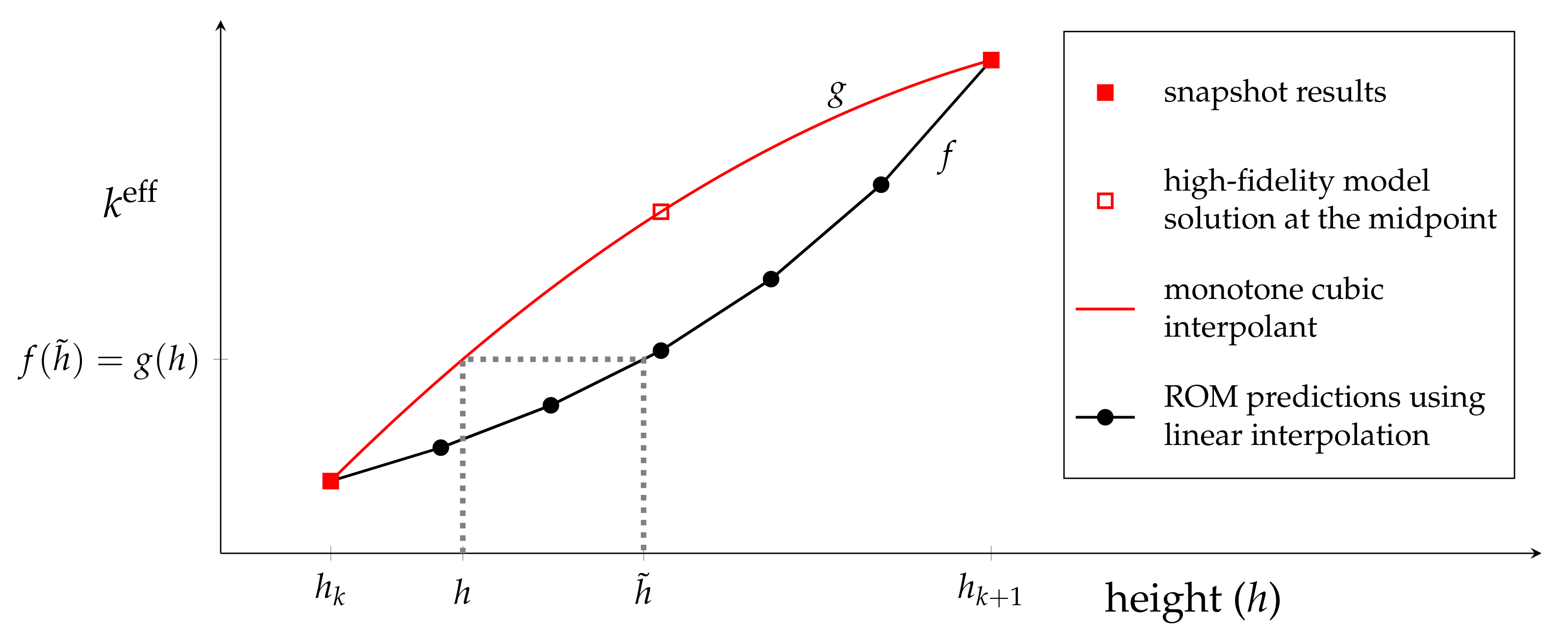
To alleviate this, we introduce nonlinear interpolation in place of linear interpolation in Equation (28), affecting Equations (27) and (37), which give the interpolation for control-rod height for the global and local ROMs, respectively. As before, the snapshots are generated, an SVD is taken, a POD basis is constructed, and the reduced matrices are formed. Ordinarily, this would complete the offline stage and would give us the building blocks of the reduced-order model. To obtain the improvement in the modelling of the control-rod height by the reduced-order model, we introduce this additional step. A set of high-fidelity model solutions is generated at heights in between the control-rod heights that are used in the training of the model. This allows a smooth representation of k eff to be constructed between each pair of snapshots. In this case, we use cubic interpolation, and therefore, a piecewise cubic interpolant, g ( h ) , represents k eff over the whole range of control-rod height. In order to preserve the monotonicity of the data in the curve, we use a piecewise cubic Hermite interpolant proposed by Fritsch and Carlson [39] specifically designed to give a piecewise monotonic curve. In this case, only three data points are required. The reduced-order model is run, linearly interpolating between the control-rod heights as before, resulting in a curve f ( h ) . By comparing the ROM results with the piecewise cubic curve, we are able to determine a nonlinear map (see Figure 2). For any height h, we find the value on the cubic interpolant corresponding to this height, g ( h ) . We then find h ˜ such that the piecewise linear representation of the ROM results takes the value f ( h ˜ ) , i.e., find h ˜ such that g ( h ) = f ( h ˜ ) . In our linear interpolation, we use h ˜ in place of h. We therefore rewrite Equation (28) as
α ( h ) = h k + 1 h ˜ ( h ) h k + 1 h k .
Such a mapping could be found for each temperature profile used in the training of the model; however, this was found not to be necessary.

4. Results

4.1. Problem Set-Up

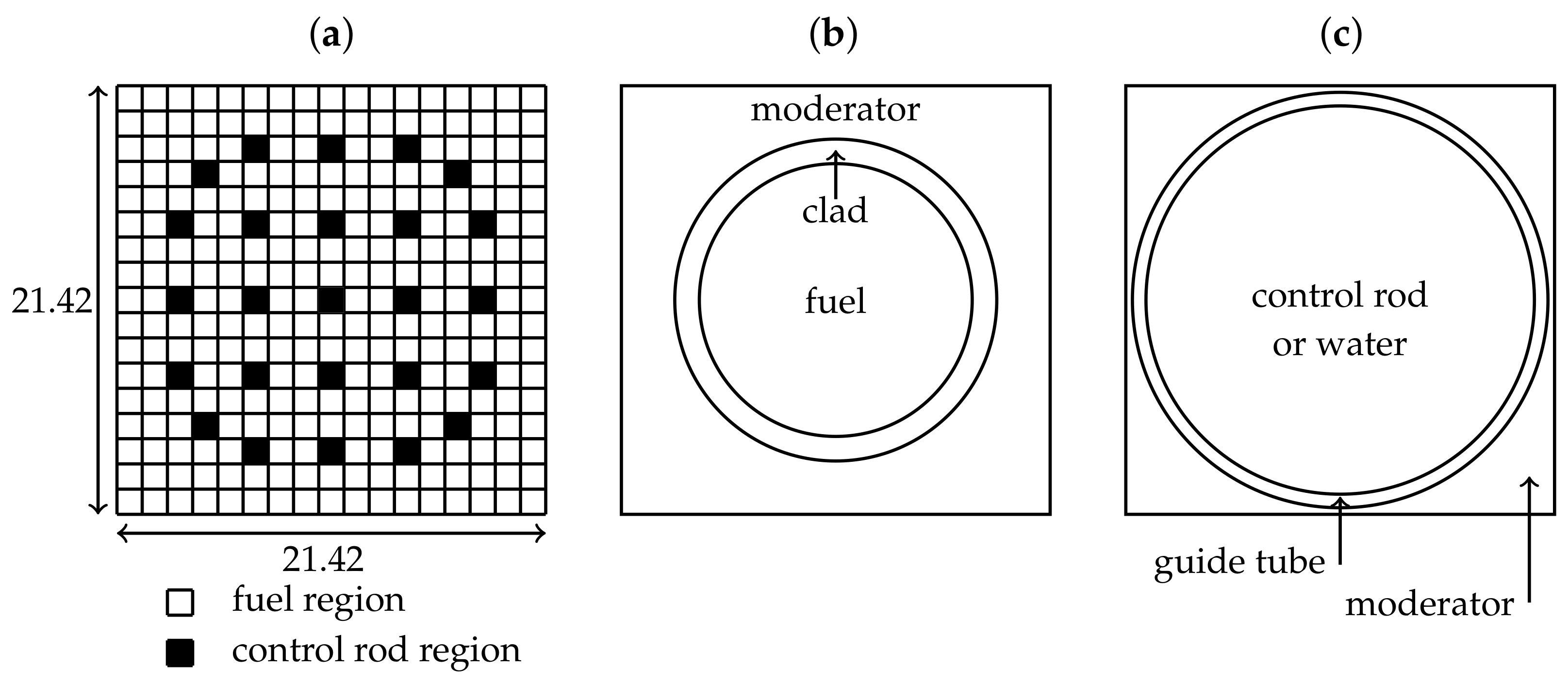
To investigate the reduced-order models presented in the previous section, a fuel assembly of a pressurised water reactor (PWR) is chosen as a test case. Reflective boundary conditions are applied to the sides of the assembly to model the presence of neighbouring assemblies that would be found in a reactor core. Void boundary conditions are applied to the top and bottom of the fuel assembly. Figure 3a shows an array of 17 × 17 channels, comprising 264 fuel pins and 25 control rods. Figure 3b shows the fuel region, consisting of fuel (uranium, enriched 2.4 %   U 235 ) of radius r = 0.4025   c m surrounded by cladding (zirconium and chromium) of width 0.0725   c m and a moderator (water), which also acts as a coolant. As shown in Figure 3c, the control-rod region houses the control rod, unless withdrawn, in which case the channel is filled with water. The control rod, of radius r = 0.573   c m , is inside a guide tube of width r = 0.04   c m , again surrounded by water. Each channel has a total size of 1.265   c m by 1.265   c m . The material cross-sections were calculated with WIMS [43] and smeared so that there is one value for each cross-section per energy group (see Table 1).
The high-fidelity model simulations were run with FETCH2, a code which solves the Boltzmann transport equations for the neutron population [2,46], developed by the Applied Modelling and Computation Group at Imperial. Here, we use FETCH2 to solve the multigroup criticality diffusion equation for a two energy-group problem. Eight-noded hexahedral elements with four quadrature points were used in the finite element discretisation. The mesh had 17 by 17 by 60 elements over a domain of [ 0 , 21.42 ] × [ 0 , 21.42 ] × [ 0 , 300 ] ( c m ) , and, when taking into account the two energy groups, this makes 39,528 degrees of freedom. The reduced-order models were constructed and solved in python using PETSc4py [47] and SLEPc4py [48].

4.2. Error Norms

In order to assess the results, we define an error measure similar to a discrete L 2 norm and infinity norm for k eff , and a discrete L 2 norm for the scalar flux profiles. For a given temperature profile, the two error measures for k eff are
e 2 = i ( k eff ) i ( k R O M eff ) i 2 i ( k eff ) i 2 and e = max i ( k eff ) i ( k R O M eff ) i ,
where k eff is the value from the high-fidelity model (which is taken as the exact or correct value), k R O M eff is the approximation of the reduced-order model, and i indicates the control-rod height. For the scalar flux, the discrete L 2 norm of the flux error for a given temperature profile, θ j , is defined as
e 2 ϕ = 1 G N h g = 1 G k = 1 N h ϕ g ( θ j , h k ) ϕ g ( θ j , h k ) R O M 2 ϕ g ( θ j , h k )
where an average is taken over the error at each particular control-rod height ( h k ) to be considered, and over the G energy groups. There are N h control-rod heights considered in this definition. The L 2 and infinity norms are defined [49] as follows:
u v 2 = 1 N i = 1 N u i v i 2
u = max i | u i |
where N is the number of nodes, and u and v are vectors of length N.

4.3. Comparing Results from the Reduced Model Algorithms

We now present results for the two algorithms, global POD and local POD, proposed in Section 3.2.1 and Section 3.2.2, respectively.

4.3.1. Global Proper Orthogonal Decomposition

In generating the snapshots for Global POD (GPOD), the following temperatures and control-rod heights were used
θ ( z ) { 291 , 1398 } ( C ) h { 0 , 10 , 20 , , 280 , 290 , 300 } ( c m ) .
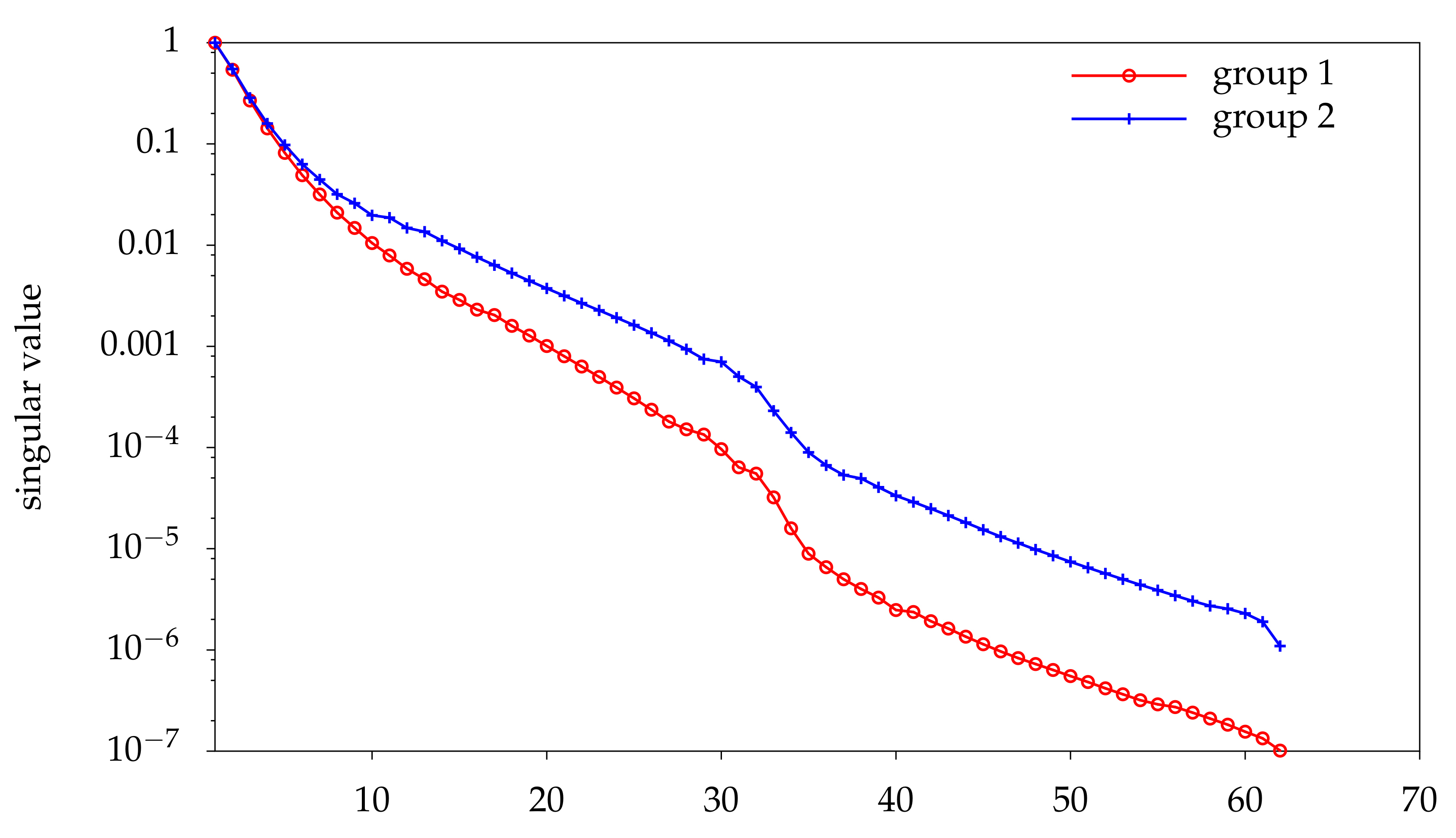
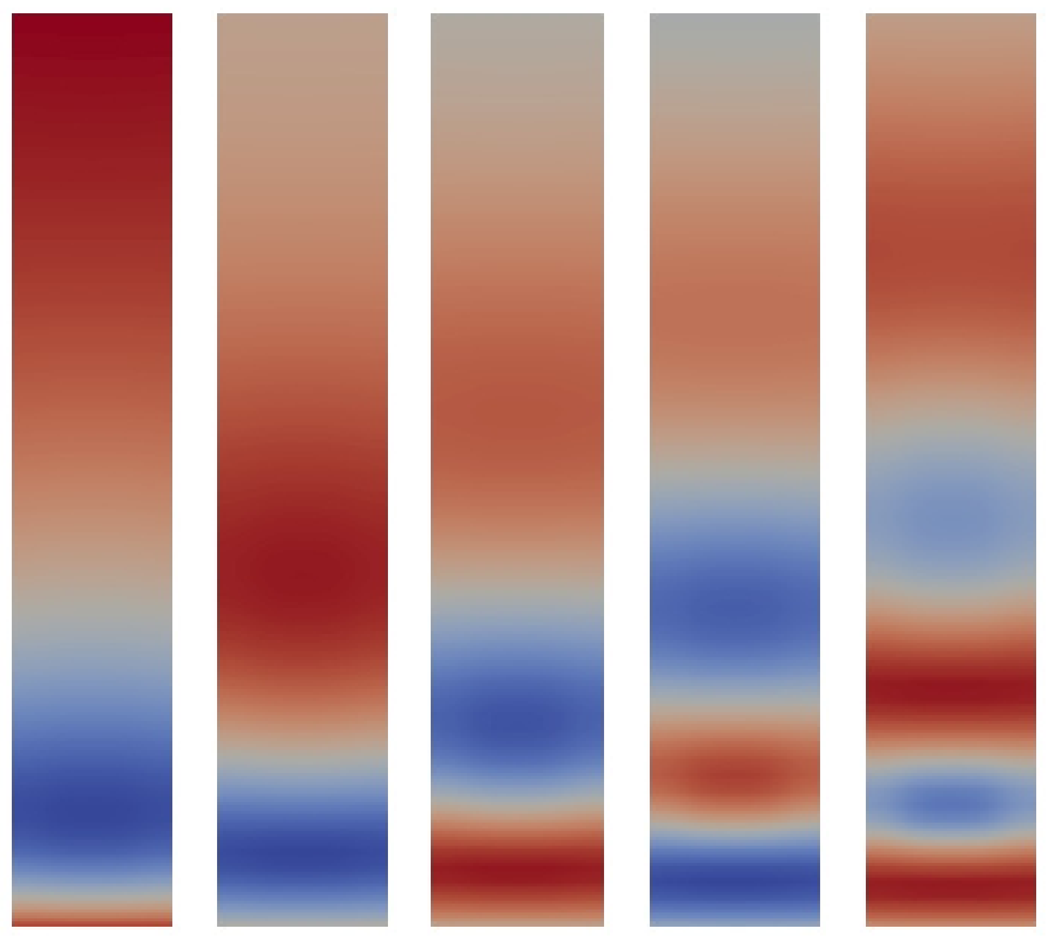
The temperature profiles are uniform in z, are applied to all regions (fuel or control rod), and correspond to temperatures for which the cross-sections are known. Once the solutions to the high-fidelity model are known for the 62 combinations of the above parameters, the POD basis functions can be calculated by applying singular value decomposition to the snapshots matrix. In order to select the most important basis functions, a tolerance of η = 0.99995 was used (see Equation (15)). This resulted in selecting 17 of a possible 62 basis functions for group 1 and 25 of a possible 62 for group 2, corresponding to capturing 99.9995% of the information of all 124 basis functions. The decay of the singular values is shown in Figure 4 and the first five POD basis functions for the group 2 scalar flux can be seen in Figure 5. It can be seen that the basis functions identified discontinuities that will have been present in the snapshots.
The next stage is to project the matrices of the high-fidelity model for each set of parameters onto the POD basis functions, and for 10 layers, this results in 1240 matrices:
A R ( θ j , h k , ) , B R ( θ j , h k , ) R 42 × 42
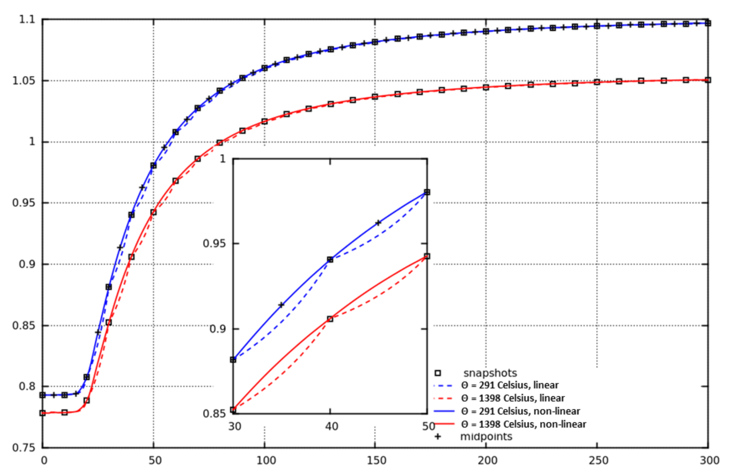
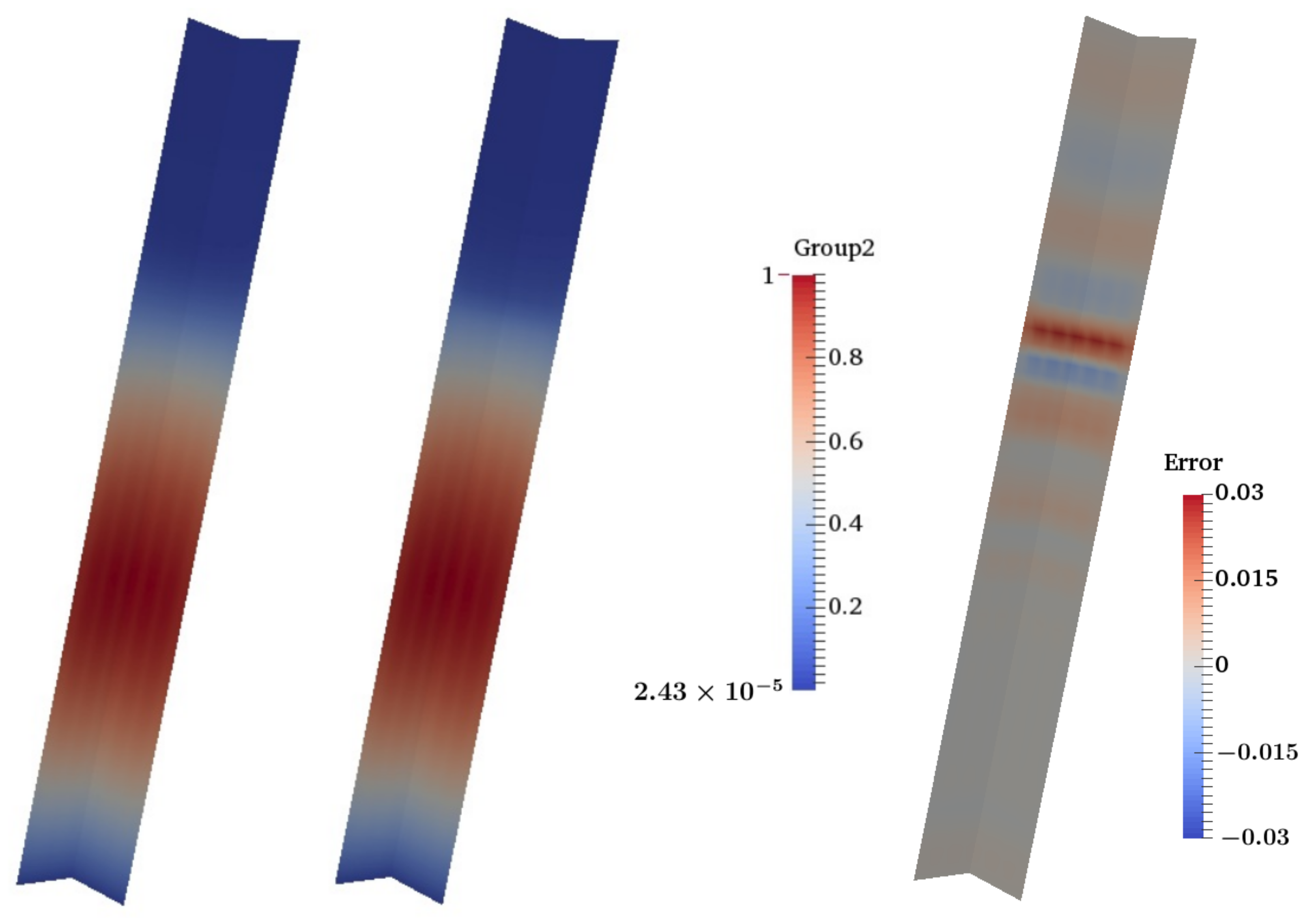
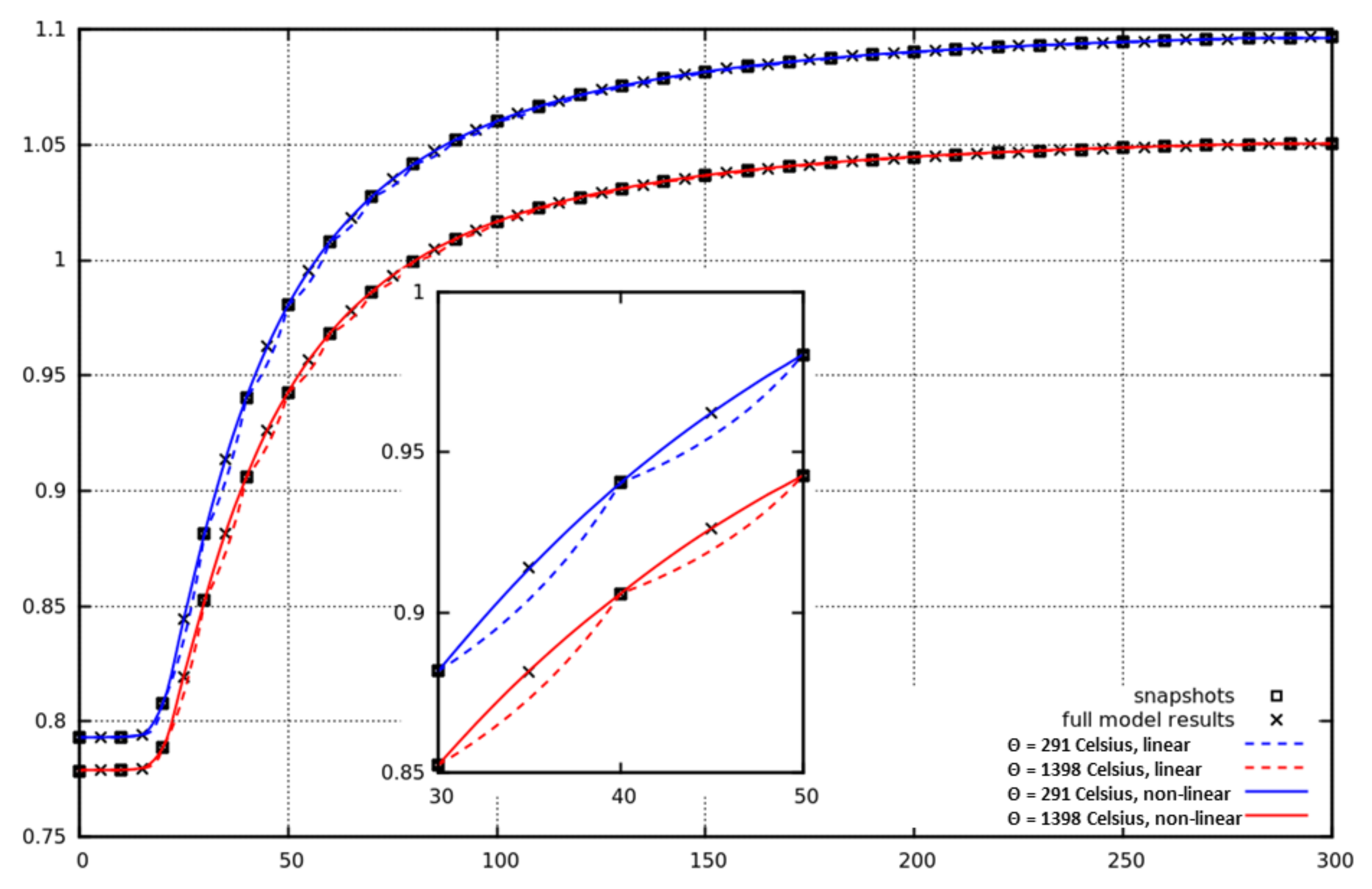
for integers j , k , , where j [ 1 , 2 ] , k [ 1 , 31 ] , [ 1 , 10 ] . We are now in a position to run the reduced-order model. The two temperature fields used to train the model (i.e., the seen temperature fields) were applied in turn and the control-rod height was sampled at 1   c m intervals from fully inserted ( z = 0   c m ) to fully withdrawn ( z = 300   c m ). At 10   c m intervals, the reduced-order model parameters will coincide with those used in training the model. In Figure 6, the dotted lines represent k eff from the reduced-order model based on GPOD and linear interpolation. This shows good agreement with the values from the high-fidelity model when the parameters coincide with the those used in training. In between these points, the ROM prediction of k eff is less accurate. This is due to the approximation involved in assembling the reduced system of equations by interpolating from matrices associated with the closest parameters. The interpolation process leads to an under-estimation of k eff due to the strong effect of absorption coefficients. This effect can be mitigated by applying the nonlinear interpolation as described in Section 3.3. When applying this interpolation, the results from the reduced-order model (solid lines) show good agreement as to whether the control-rod height corresponds to a seen or an unseen value. Figure 7 compares the scalar flux from the high-fidelity model with that of the reduced-order model for a control rod inserted to a depth of 205   c m and temperature of 291 °C, thus the control-rod height is unseen but the temperature profile is seen. The pointwise error is shown on the right, revealing that the largest error occurs near the base of the control rod, which is to be expected as the flux profile changes abruptly in this region. The agreement between the high-fidelity model and the reduced-order model is very good.
We now wish to see how well the reduced-order model behaves for both unseen temperature profiles and unseen control-rod heights. We use two unseen temperature profiles, one uniform and one sinusoidal:
θ = 800 ° C
θ ( z ) = 600 + 400 sin π z L ( ° C )
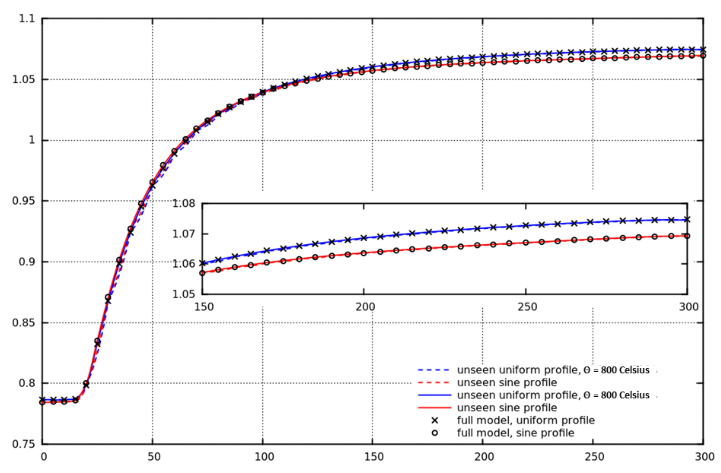
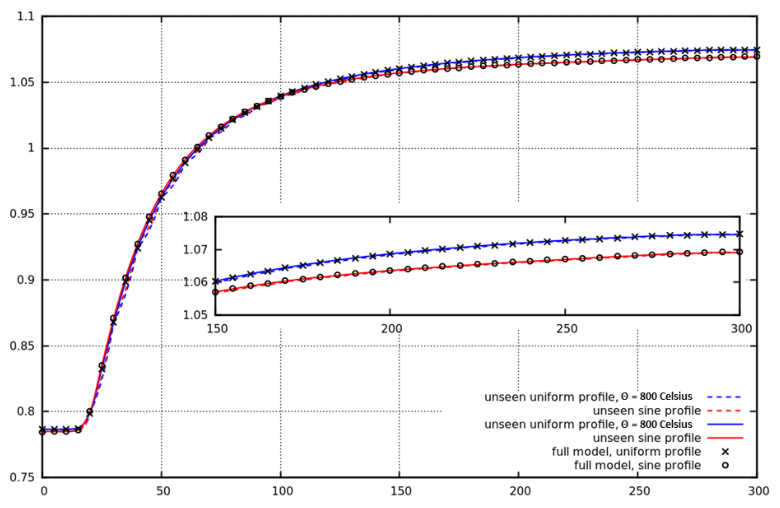
where L is the length of the reactor. The prediction of k R O M eff by the reduced-order model based on GPOD and linear interpolation is represented by the dotted line in Figure 8. The solid line again represents the prediction of the reduced-order model based on using nonlinear interpolation. The agreement when using the map is excellent.
Table 2 shows the error in predicting k eff and the scalar flux by the reduced-order models using the definitions given in Equations (43) and (44). The error is first calculated for a known temperature profile ( θ = 291 ° C ) at the known control-rod heights given in Equation (47). In this case, the error is less than when the error is calculated at 5   c m intervals (which will include some unseen rod heights). This is expected after inspection of Figure 6, which shows the largest difference between the high-fidelity model and the predictions from the ROM based on GPOD occurs when the control-rod height is unseen. The nonlinear interpolation reduces the error considerably when the error is calculated at unseen points. For k eff , there is a reduction in the error of two orders of magnitude, and for the flux, there is a reduction of one order of magnitude. Table 3 shows the error measures applied to k eff and the scalar flux for unseen control-rod heights and temperature profiles. For the unseen parameters, the nonlinear interpolation method has errors that are again two orders of magnitude lower than the errors associated with the linear interpolation for k eff and one order of magnitude lower for the scalar flux.

4.3.2. Local Proper Orthogonal Decomposition

The reduced-order model resulting from GPOD gives excellent agreement with the high-fidelity model. However, the more snapshots are used, the larger the number of basis functions can be, which leads to longer times taken in the projection stage and larger reduced systems. This issue motivated the development of a second method which has multiple bases, each corresponding to a subset of parameter space.
In constructing the reduced model local POD (LPOD) outlined in Section 3.2.2, we used the same parameter sets (and therefore, the same snapshots) as in GPOD (see Equation (47)). To impose varying temperature profiles in the reduced-order model, the domain was split into vertical layers, just as for GPOD. Furthermore, we now assign a particular set of basis functions to each layer. In this example, each layer has a height of 30   c m , which means there are snapshots associated with 4 rod heights in each layer. For a layer , we take an SVD of the following snapshots
ϕ ( θ j , h k ) j = 1 2 k = 1 + 3 ( 1 ) , 4 + 3 ( 1 )
that is, in each layer, we take the SVD of 8 of the 62 snapshots. For example, for layer 1, the set of snapshots used is
ϕ ( θ j , h k ) j = 1 N θ = 2 k = 1 4 = ϕ ( θ 1 , h 1 ) , ϕ ( θ 2 , h 1 ) , ϕ ( θ 1 , h 2 ) , ϕ ( θ 2 , h 2 ) , ϕ ( θ 1 , h 3 ) , ϕ ( θ 2 , h 3 ) , ϕ ( θ 1 , h 4 ) , ϕ ( θ 2 , h 4 ) .
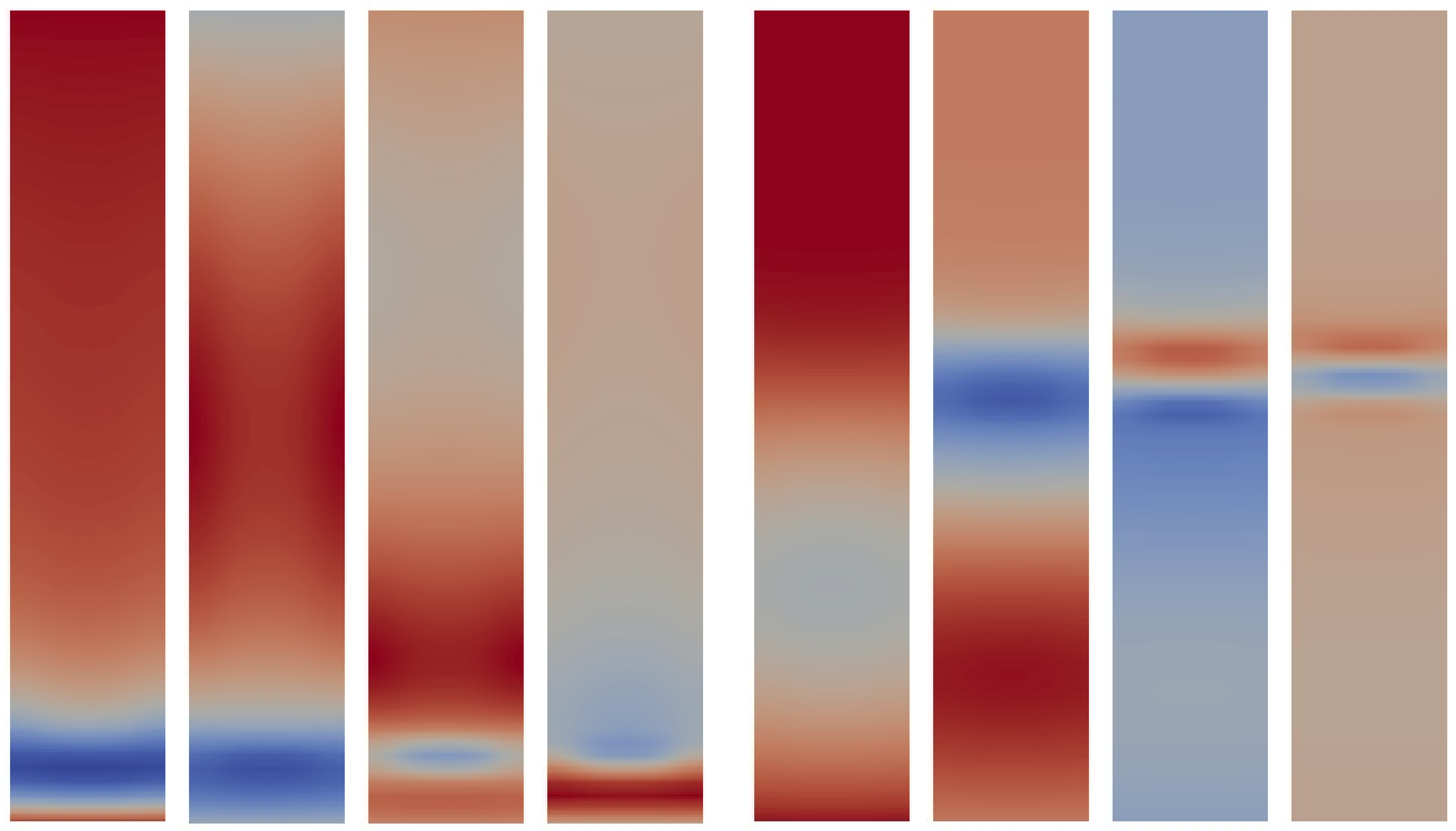
For each layer, therefore, we have a maximum of eight basis functions for each group. In total, this gives a maximum of 80 basis functions per group; however, only a maximum of eight would be used to construct a ROM for a given rod height and temperature profile (see Figure 1). Figure 9 shows the singular values for the each layer. Figure 10 shows the first four POD basis functions associated with group 2 for when the control rod is inserted to somewhere within the lowest vertical layer, layer 1 z [ 0 , 30 ] , and when the control rod is inserted to somewhere within the layer just above the central point, layer 6, z [ 150 , 180 ] . By comparison with Figure 5, one can see that the POD basis functions for LPOD capture sharper features from the snapshots.
As for GPOD, we use a tolerance of 0.999995 to select the basis functions, resulting in between three and six basis functions in each layer per group (see Table 4). Projecting the high-fidelity model matrices onto the basis functions results in 1600 matrices
A ( 1 , 2 ) R ( θ j , h k , ) , B ( 1 , 2 ) R ( θ j , h k , ) R n × n
for integers j , k , 1 , 2 , where j [ 1 , 2 ] , k [ 1 , 31 ] , 1 , 2 [ 1 , 10 ] . Here n , the total number of basis functions per layer, takes a value between 6 and 11: see Table 4 for the number of basis functions for each layer and each energy group. As we interpolate within layers, we do not have the problem of interpolating between differently sized matrices.
As before, we run the reduced-order model for the known temperatures sampling the control-rod height at 1   c m intervals over the full range of the assembly. Plots of k R O M eff predicted by the LPOD-based ROM can be seen in Figure 11. Both linear and nonlinear interpolation are used, and again, the nonlinear interpolation significantly improves the results. The error norms defined in Equations (43) and (44) are calculated (using high-fidelity model results found at 5   c m intervals) and the results can be seen in Table 5. The errors in both k eff and the scalar fluxes are lower when using the nonlinear interpolation method.
To investigate how the reduced-order model behaves for unseen parameters, the two temperature profiles in Equation (48) are used and the control-rod height is sampled at 1   c m intervals. Figure 12 shows plots of k eff against control-rod height. The agreement is very good for the unseen uniform profile, and reasonable for the unseen sinusoidal profile. Error norm values in Table 6 show that the nonlinear interpolation improves the accuracy of the values of k R O M eff and the accuracy of the scalar fluxes. When using nonlinear interpolation, the accuracy of the prediction of k eff for unseen parameters can match the accuracy of the prediction for the seen parameters, and the errors in the scalar flux are reduced by one order of magnitude.
Now consider the computing times. The time taken by WIMS to calculate the cross-sections for these problems was in the order of minutes, and therefore does not contribute significantly to the offline computation time. Table 7 shows the time taken to generate each snapshot as being 499 s, whereas the time taken by the reduced-order model to solve one problem and reconstruct the scalar flux field is approximately 0.004 s for GPOD and 0.003 s for LPOD. The computational speed-up is defined as
time for one high - fidelity model calculation time for a ROM calculation
which is in the order of 120,000 for GPOD and 150,000 for LPOD. We remark that this figure depends on the efficiency of the high-fidelity model, and improving this would decrease the speeding up. However, this would not be expected to make more than one or two orders of magnitude difference, so the speeding up is would still be significant and the time taken to solve the ROM clearly points to the potential of both methods proposed here to be able to predict in real time.
For both the global and local methods described here, many small matrices are written to disk during the offline stage. For the global method, these matrices are of the dimensions 42 by 42, so each matrix requires 42 × 42 × 8 = 14,112 bytes of space, as one double precision (or 64 bit) real number is stored in 8 bytes. Assuming that 1 MB ≡ 1024 2 bytes, the 1240 matrices occupy about 17 MB of disk space in total. For the local method, more matrices are written to disk, however these matrices are smaller, varying from 6 by 6 to 11 by 11 (see Table 4) and, therefore, take less disk space than those of the global method.

5. Discussion and Conclusions

Two reduced-order models (ROMs) have been proposed in this paper. The first generates a set of snapshots by varying control-rod height and temperature, from which is derived a set of POD basis functions (global POD or GPOD) [32]. Standard Galerkin projection is applied to approximate the system for unseen parameter values. The second, a new approach, uses snapshots with similar control-rod heights to form one of a number of sets of basis functions (local POD or LPOD), which are, therefore, local in the parameter space associated with the control-rod height. The latter method makes use of vertical layers and forms a set of POD basis functions in each layer based on snapshots generated by control-rod heights that lie within the layer. All the high-fidelity system matrices associated with control-rod heights within a particular layer and all temperature profiles are projected onto the different sets of basis functions. These form a set of pre-calculated or pre-determined reduced system matrices that are used as building blocks in the online stage, which assembles reduced system matrices for unseen parameter values by interpolating the pre-calculated matrices. For an unseen control-rod height, the basis functions are chosen according to the layer that the unseen rod height falls within. For both the GPOD-based ROM and LPOD-based ROM, two interpolation schemes are used to model the dependence on control-rod height: a linear interpolation and a novel nonlinear interpolation, which uses a piecewise cubic Hermite interpolant [39] to give a monotonic curve ideal for the description of k eff . To generate the monotonic interpolant, an additional set of high-fidelity model solutions at midpoints of the seen control-rod heights for one temperature profile are generated. This increases the cost of the offline stage, but significantly increases the accuracy of the results with regard to the interpolation of control-rod height. Linear interpolation is used to model the dependence on temperature.
To demonstrate the methods proposed here, snapshots are generated with FETCH2 [2] of a PWR fuel assembly. Two constant temperature profiles and 31 control-rod heights are used to generate the snapshots. For the reduced-order model based on GPOD, the error norms of scalar flux and k eff are lowest when replicating the seen parameter values, as expected. For unseen control-rod heights and temperature profiles, when using nonlinear interpolation to model the control-rod movement, the error in k eff is reduced by two orders of magnitude, from O ( 10 3 ) to O ( 10 5 ) , and the error in the scalar flux is reduced by one order of magnitude, from O ( 10 2 ) to O ( 10 3 ) . Similar behaviour and error reductions are found for the reduced-order model based on LPOD. The reduced-order model based on GPOD uses 42 basis functions to achieve a given level of accuracy, whereas, for the same level of accuracy, the model based on LPOD requires between three and six basis functions per layer, resulting in the latter running slightly faster.
For further work, it would be interesting to apply the local and global methods to more complex problems to see if the more abruptly changing basis functions obtained in the former method prove significant. Coupling the reduced-order models with a thermal hydralics code would also add realism to the solutions, providing a mechanism to solve these problems with physical temperature profiles.
In conclusion, the global and local reduced-order models perform similarly well, although the basis functions of the local method are able to represent more abrupt changes in the flux solution. When replicating results for the seen parameter values of control-rod height and temperature, both global and local reduced-order models give accurate results for k eff with either linear or nonlinear interpolation. For unseen values, the nonlinear method of interpolation outperforms the linear method, finding an error in k eff similar to that for the seen values and two orders of magnitude lower than for linear interpolation. For the scalar flux, using nonlinear interpolation reduces the error by one order of magnitude for both the global and local methods. Although the local reduced-order model is slightly faster, the solution times of both models show the potential of these methods to be able to predict in real time.

Author Contributions

In producing this manuscript, the following contributions have been made: conceptualization, A.G.B., C.C.P. and S.J.; methodology, all authors.; software, C.E.H., A.G.B.; writing—original draft preparation, C.E.H.; writing—review and editing, all authors; funding acquisition, S.J. and A.G.B. All authors have read and agreed to the published version of the manuscript.

Funding

The authors gratefully acknowledge financial support from the Defence Academy at HMS Sultan through the grant Computational Nuclear Engineering Research. A.G.B acknowledges support from the EPSRC Fellowship EP/M022684/1. C.C.P and C.E.H would also like to acknowledge the EPSRC grants MUFFINS (EP/P033180/1); PREMIERE (EP/T000414/1); RELIANT (EP/V036777/1); and INHALE (EP/T003189/1).

Institutional Review Board Statement

Not applicable.

Informed Consent Statement

Not applicable.

Data Availability Statement

The data presented in this study are available on request from the corresponding author.

Acknowledgments

The authors would like to acknowledge insightful discussions with Paul N. Smith, Richard Smedley-Stevenson and Alan V. Jones, and Steven Dargaville whilst undertaking this study. Furthermore, the authors are grateful to the reviewers for their detailed comments which have improved the paper.

Conflicts of Interest

The authors declare no conflict of interest.

References

  1. Buchan, A.G.; Dargaville, S.; Pain, C.C. A combined immersed body and adaptive mesh method for simulating neutron transport within complex structures. Ann. Nucl. Energy 2019, 134, 88–100. [Google Scholar] [CrossRef]
  2. Dargaville, S.; Goffin, M.A.; Buchan, A.G.; Pain, C.C.; Smedley-Stevenson, R.P.; Smith, P.N.; Gorman, G. Solving the Boltzmann transport equation with multigrid and adaptive space/angle discretisations. Ann. Nucl. Energy 2015, 86, 99–107. [Google Scholar] [CrossRef]
  3. Dargaville, S.; Buchan, A.G.; Smedley-Stevenson, R.P.; Smith, P.N.; Pain, C.C. Scalable angular adaptivity for Boltzmann transport. J. Comput. Phys. 2020, 406, 109124. [Google Scholar] [CrossRef] [Green Version]
  4. Davidson, G.G.; Evans, T.M.; Jarrell, J.J.; Hamilton, S.P.; Slaybaugh, R.N. Massively Parallel, Three-Dimensional Transport Solutions for the k-Eigenvalue Problem. Nucl. Sci. Eng. 2014, 177, 111–125. [Google Scholar] [CrossRef]
  5. Slaybaugh, R.N.; Ramirez-Zweiger, M.; Pandya, T.; Hamilton, S.; Evans, T.M. Eigenvalue Solvers for Modeling Nuclear Reactors on Leadership Class Machines. Nucl. Sci. Eng. 2018, 190, 31–44. [Google Scholar] [CrossRef] [Green Version]
  6. Schilders, W.H.A.; van der Vorst, H.A.; Rommes, J. (Eds.) Model order reduction: Theory, research aspects and applications. In The European Consortium for Mathematics in Industry; Springer: Berlin, Germany, 2008; Volume 13. [Google Scholar]
  7. Chinesta, F.; Leygue, A.; Bordeu, F.; Aguado, J.V.; Cueto, E.; Gonzalez, D.; Alfaro, I.; Ammar, A.; Huerta, A. PGD-Based Computational Vademecum for Efficient Design, Optimization and Control. Arch. Comput. Methods Eng. 2013, 20, 31–59. [Google Scholar] [CrossRef]
  8. Zahr, M.J.; Farhat, C. Progressive construction of a parametric reduced-order model for PDE-constrained optimization. Int. J. Numer. Methods Eng. 2015, 102, 1111–1135. [Google Scholar] [CrossRef] [Green Version]
  9. Niroomandi, S.; Alfaro, I.; Gonzalez, D.; Cueto, E.; Chinesta, F. Real-time simulation of surgery by reduced order modelling and X-FEM techniques. Int. J. Numer. Methods Biomed. Eng. 2011, 28, 574–588. [Google Scholar] [CrossRef] [PubMed] [Green Version]
  10. Aguado, J.V.; Huerta, A.; Chinesta, F.; Cueto, E. Real-time monitoring of thermal processes by reduced-order modeling. Int. J. Numer. Methods Eng. 2015, 102, 991–1017. [Google Scholar] [CrossRef]
  11. Benner, P.; Gugercin, S.; Willcox, K. A Survey of Projection-Based Model Reduction Methods for Parametric Dynamical Systems. SIAM Rev. 2015, 57, 483–531. [Google Scholar] [CrossRef]
  12. Rheinboldt, W.C. On the Theory and Error Estimation of the Reduced Basis Method for Multi-Parameters Problems. Nonlinear Anal. Theory Methods Appl. 1993, 21, 849–858. [Google Scholar] [CrossRef]
  13. Hesthaven, J.S.; Stamm, B.; Zhang, S. Efficient greedy algorithms for high-dimensional parameter spaces with applications to empirical interpolation and reduced basis methods. ESAIM M2AN 2014, 48, 259–283. [Google Scholar] [CrossRef] [Green Version]
  14. Quarteroni, A.; Manzoni, A.; Negri, F. Reduced Basis Methods for Partial Differential Equations: An Introduction; Springer International Publishing: Berlin, Germany, 2016. [Google Scholar]
  15. Rozza, G.; Huynh, D.B.P.; Patera, A.T. Reduced Basis Approximation and a Posteriori Error Estimation for Affinely Parametrized Elliptic Coercive Partial Differential Equations. Arch. Comput. Methods Eng. 2008, 15. [Google Scholar] [CrossRef] [Green Version]
  16. Siddiqui, M.S.; Fonn, E.; Kvamsdal, T.; Rasheed, A. Finite-Volume High-Fidelity Simulation Combined with Finite-Element-Based Reduced-Order Modeling of Incompressible Flow Problems. Energies 2019, 12, 1271. [Google Scholar] [CrossRef] [Green Version]
  17. Castagna, C.; Aufiero, M.; Lorenzi, S.; Lomonaco, G.; Cammi, A. Development of a Reduced Order Model for Fuel Burnup Analysis. Energies 2020, 13, 890. [Google Scholar] [CrossRef] [Green Version]
  18. Sirovich, L. Turbulence and the dynamics of Coherent Structures. Part 1: Coherent Structures. Q. Appl. Math. 1987, 45, 561–571. [Google Scholar] [CrossRef] [Green Version]
  19. Holmes, P.; Lumley, J.L.; Berkooz, G.; Rowley, C.W. Turbulence, Coherent Structures, Dynamical Systems and Symmetry; Cambridge University Press: Cambridge, UK, 2012. [Google Scholar]
  20. Taira, K.; Brunton, S.L.; Dawson, S.T.M.; Rowley, C.W.; Colonius, T.; McKeon, B.J.; Schmidt, O.T.; Gordeyev, S.; Theofilis, V.; Ukeiley, L.S. Modal Analysis of Fluid Flows. AIAA J. 2017, 55, 4013–4041. [Google Scholar] [CrossRef] [Green Version]
  21. Lucia, D.J.; King, P.I.; Beran, P.S. Reduced order modeling of a two-dimensional flow with moving shocks. Comput. Fluids 2003, 32, 917–938. [Google Scholar] [CrossRef]
  22. Lee, K.; Carlberg, K.T. Model reduction of dynamical systems on nonlinear manifolds using deep convolutional autoencoders. J. Comput. Phys. 2020, 404, 108973. [Google Scholar] [CrossRef] [Green Version]
  23. Ahmed, S.E.; Rahman, S.M.; San, O.; Rasheed, A.; Navon, I.M. Memory embedded non-intrusive reduced order modeling of non-ergodic flows. Phys. Fluids 2019, 31, 126602. [Google Scholar] [CrossRef] [Green Version]
  24. Phillips, T.R.F.; Heaney, C.E.; Smith, P.N.; Pain, C.C. An autoencoder-based reduced-order model for eigenvalue problems with application to neutron diffusion. Int. J. Numer. Methods Eng. 2020. preprint. [Google Scholar]
  25. Buchan, A.G.; Pain, C.C.; Fang, F.; Navon, I.M. A POD reduced-order model for eigenvalue problems with application to reactor physics. Int. J. Numer. Methods Eng. 2013, 95, 1011–1032. [Google Scholar] [CrossRef] [Green Version]
  26. Sartori, A.; Cammi, A.; Luzzi, L.; Rozza, G. A Reduced Basis Approach for Modeling the Movement of Nuclear Reactor Control Rods. J. Nucl. Eng. Radiat. Sci. 2016, 2, 1–8. [Google Scholar] [CrossRef]
  27. Sartori, A.; Cammi, A.; Luzzi, L.; Rozza, G. Reduced Basis Approaches in Time-Dependent Non-Coercive Settings for Modelling the Movement of Nuclear Reactor Control Rods. Commun. Comput. Phys. 2016, 20, 23–59. [Google Scholar] [CrossRef] [Green Version]
  28. Zhang, C.; Chen, G. Fast solution of neutron diffusion problem by reduced basis finite element method. Ann. Nucl. Energy 2018, 111, 702–708. [Google Scholar]
  29. Zhang, C.; Chen, G. Fast solution of neutron transport SP3 equation by reduced basis finite element method. Ann. Nucl. Energy 2018, 120, 707–714. [Google Scholar] [CrossRef]
  30. Gong, H.; Chen, W.; Zhang, C.; Chen, G. Fast solution of neutron diffusion problem with movement of control rods. Ann. Nucl. Energy 2020, 149, 107814. [Google Scholar]
  31. Heaney, C.E.; Buchan, A.G.; Pain, C.C.; Jewer, S. A reduced order model for criticality problems in reactor physics varying control rod settings. In Proceedings of the 24th Conference on Computational Mechanics; Jefferson, A., Kerfriden, P., Eds.; ACME-UK: Cardiff, UK, 2016; pp. 327–330. [Google Scholar]
  32. Heaney, C.E.; Buchan, A.G.; Pain, C.C.; Jewer, S. Reactor Simulators and Reduced Order Modelling. Nuclear Future 2018, 14, 49–54. [Google Scholar]
  33. German, P.; Ragusa, J.C. Reduced-order modeling of parameterized multi-group diffusion k-eigenvalue problems. Ann. Nucl. Energy 2019, 134, 144–157. [Google Scholar] [CrossRef]
  34. Lorenzi, S. An Adjoint Proper Orthogonal Decomposition method for a neutronics reduced order model. Ann. Nucl. Energy 2018, 114, 245–258. [Google Scholar] [CrossRef]
  35. Choi, Y.; Brown, P.; Arrighi, W.; Anderson, R.; Huynh, K. Space-time reduced order model for large-scale linear dynamical systems with application to Boltzmann transport problems. J. Comput. Phys. 2021, 424, 109845. [Google Scholar] [CrossRef]
  36. Jamelot, E.; Ciarlet, P., Jr. Fast non-overlapping Schwarz domain decomposition methods for solving the neutron diffusion equation. J. Comput. Phys. 2013, 241, 445–463. [Google Scholar] [CrossRef]
  37. Cherezov, A.; Sanchez, R.; Joo, H.G. A reduced-basis element method for pin-by-pin reactor core calculations in diffusion and SP3 approximations. Ann. Nucl. Energy 2018, 116, 195–209. [Google Scholar] [CrossRef]
  38. Phillips, T.R.F.; Heaney, C.E.; Tollit, B.S.; Smith, P.N.; Pain, C.C. Reduced-Order Modelling with Domain Decomposition Applied to Multi-Group Neutron Transport. Energies 2021. accepted for publication. [Google Scholar]
  39. Fritsch, F.N.; Carlson, R.E. Monotone Piecewise Cubic Interpolation. SIAM J. Numer. Anal. 1980, 17, 238–246. [Google Scholar] [CrossRef]
  40. Cho, N. Fundamentals and Recent Developements of Reactor Physics Methods. Nucl. Eng. Technol. 2005, 37, 25–78. [Google Scholar]
  41. Yoon, J.I.; Joo, H.G. Two-Level Coarse Mesh Finite Difference Formulation with Multigroup Source Expansion Nodal Kernels. J. Nucl. Sci. Technol. 2008, 45, 668–682. [Google Scholar] [CrossRef]
  42. Munoz-Cobo, J.; Miró, R.; Wysocki, A.; Soler, A. 3D calculation of the lambda eigenvalues and eigenmodes of the two-group neutron diffusion equation by coarse-mesh nodal methods. Prog. Nucl. Energy 2019, 110, 393–409. [Google Scholar] [CrossRef]
  43. Newton, T.D.; Hutton, J.L. The next Generation WIMS Lattice Code: WIMS9. In Proceedings of the PHYSOR 2002, International Conference on the New Frontiers of Nuclear Technology, Seoul, Korea, 7–10 October 2002; Americal Nuclear Society: La Grange Park, IL, USA, 2002. [Google Scholar]
  44. Lumley, J.L. The Structure of Inhomogeneous Turbulent Flow. Atmos. Turbul. Radio Wave Propag. 1967, 166–178. [Google Scholar]
  45. Baur, U.; Benner, P.; Haasdonk, B.; Himpe, C.; Martini, I.; Ohlberger, M. Comparison of Methods for Parametric Model Order Reduction of Time-Dependent Problems. In Model Reduction and Approximation: Theory and Algorithms; Benner, P., Cohen, A., Ohlberger, M., Willcox, K., Eds.; Society for Industrial Applied Mathematics: Philadelphia, PA, USA, 2017; pp. 377–407. [Google Scholar]
  46. The FETCH Codes. Available online: www.imperial.ac.uk/earth-science/research/research-groups/amcg/software/fetch/ (accessed on 19 January 2021).
  47. Dalcin, L.; Kler, P.; Paz, R.; Cosimo, A. Parallel Distributed Computing using Python. Adv. Water Resour. 2011, 34, 1124–1139. [Google Scholar] [CrossRef]
  48. Hernandez, V.; Roman, J.E.; Vidal, V. SLEPc: A scalable and flexible tool kit for the solution of eigenvalue problems. ACM Trans. Math. Softw. 2005, 31, 351–362. [Google Scholar] [CrossRef]
  49. Langtangen, H.P.; Linge, S. Finite Difference Computing with PDEs: A Modern Software Approach; Springer: Berlin, Germany, 2017. [Google Scholar]
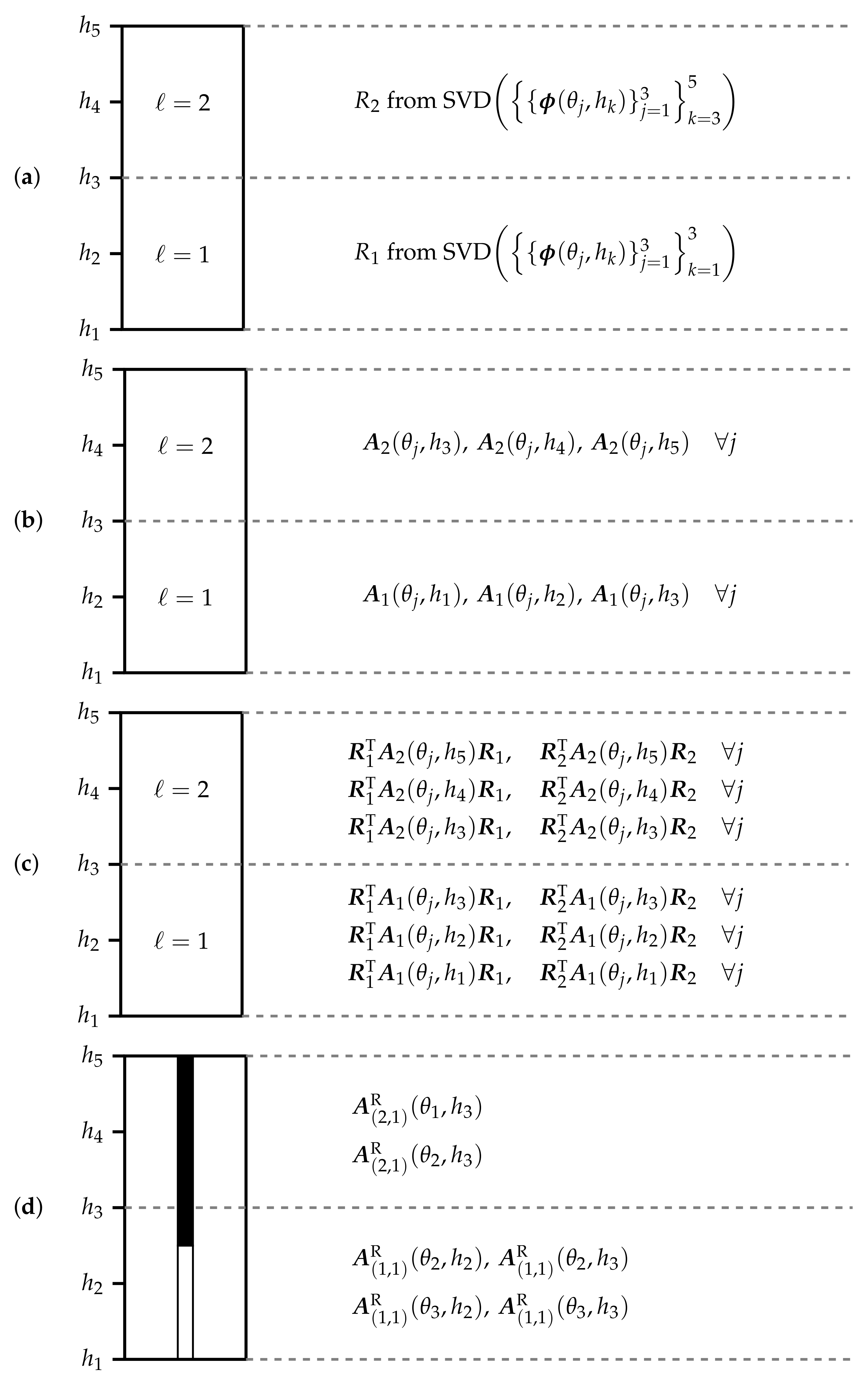
Figure 1. Suppose snapshots are taken at 5 control-rod positions { h k } k = 1 5 , at temperatures { θ j } j = 1 3 and the domain has been divided into two layers. The diagrams show (a) which snapshots are used to generate the bases at each level, (b) which full order matrices are generated, (c) which reduced-order matrices are produced by projecting the full order matrices onto the bases, (d) which reduced-order matrices are interpolated for an unseen control rod height that lies between h 2 and h 3 in layer 1 and a temperature profile whose average value for layer 1 lies in [ θ 2 , θ 3 ] , and for layer 2, in [ θ 1 , θ 2 ] . For this example, only one control rod is shown.
Energies 14 01350 g001
Figure 2. A schematic diagram of the nonlinear map. To find the weight α to be used at height h, locate h ˜ through the relationship g ( h ) = f ( h ˜ ) , where f is the piecewise linear curve passing through the ROM results and g is the (piecewise) cubic Hermitian interpolant through the high-fidelity model results.
Energies 14 01350 g002
Figure 3. (a) The array of channels in the pressurised water reactor (PWR) fuel assembly: white boxes indicate fuel regions; black boxes indicate control-rod regions. (b) The fuel region has a fuel pin (uranium, enriched 2.4 % U 235 ) of radius r = 0.4025   c m , which is surrounded by cladding (zirconium and chromium) of width 0.0725   c m and water. (c) The composition of the control-rod region. The control rod (boron and carbon) of radius r = 0.573   c m sits inside a guide tube of width r = 0.04   c m , again surrounded by water. If the rod is withdrawn, water fills the space.
Energies 14 01350 g003
Figure 4. The singular values for groups 1 and 2 associated with the scalar flux solutions (snapshots) from global proper orthogonal decomposition (GPOD). The values have been normalised by the largest singular value.
Energies 14 01350 g004
Figure 5. The first 5 Proper Orthogonal Decomposition (POD) basis functions for the group 2 scalar flux. (View of the x z plane with scaling applied in z.)
Energies 14 01350 g005
Figure 6. k eff against control-rod height. The dotted line corresponds to the reduced-order model results (GPOD) using the linear interpolation, and the solid line corresponds to the nonlinear interpolation. Two uniform temperature fields are used. For comparison, high-fidelity model results are shown, with the snapshots and midpoints (used in the nonlinear interpolation).
Energies 14 01350 g006
Figure 7. Comparison of the scalar flux (group 2) from the reduced-order model based on GPOD (left) and the high-fidelity model (centre) with the base of the control-rod at a height of 205   c m and temperature of 291 °C. The pointwise error for these group 2 solutions is shown on the right.
Energies 14 01350 g007
Figure 8. k eff against control-rod height. The dotted line corresponds to the reduced-order model results (GPOD) using the linear interpolation, and the solid line corresponds to the nonlinear interpolation. Two unseen temperature profiles are used—the first is uniform and the second sinusoidal (see Equation (48)). For comparison, high-fidelity model results are shown.
Energies 14 01350 g008
Figure 9. The singular values for groups 1 (upper) and 2 (lower) associated with the scalar flux solutions (snapshots) from local proper orthogonal decomposition. The values have been normalised by the largest singular value.
Energies 14 01350 g009
Figure 10. The first 4 POD basis functions for the group 2 scalar flux of LPOD. Leftmost plots, basis functions for layer 1 ( z [ 0 , 30 ] ) and rightmost plots, basis functions for layer 6 ( z [ 150 , 180 ] ). View of the x z plane with scaling applied in z.
Energies 14 01350 g010
Figure 11. k eff against control-rod height. The dotted line corresponds to the reduced-order model results (LPOD) using the linear interpolation, and the solid line corresponds to the nonlinear interpolation. Two uniform temperature fields are used. For comparison, high-fidelity model results are shown, with the snapshots and midpoints (used in the nonlinear interpolation).
Energies 14 01350 g011
Figure 12. k eff against control-rod height. The dotted line corresponds to the reduced-order model results (LPOD) using the linear interpolation, and the solid line corresponds to the nonlinear interpolation. Two unseen temperature profiles are used—the first is uniform and the second sinusoidal (see Equation (48)). For comparison, high-fidelity model results are shown.
Energies 14 01350 g012
Table 1. Sets of macroscopic cross-sections calculated with WIMS [43] used in the high-fidelity model.
θ = 291 °C θ = 1398 °C
Group 1Group 2Group 1Group 2
Σ a 2.771021 × 10−35.774495 × 10−22.800322 × 10−36.148412 × 10−2
Σ 1 g s 3.538874 × 10−13.651891 × 10−23.540753 × 10−13.650402 × 10−2
Fuel region Σ 2 g s 09.415292 × 10−109.378452 × 10⁻¹
Σ f 1.517885 × 10−32.457978 × 10−21.534314 × 10−32.471806 × 10−2
ν 2.756342 × 10−02.566988 × 10−02.758249 × 10−02.587363 × 10−0
χ 9.996266 × 10−13.723758 × 10−49.996268 × 10−13.723757 × 10−4
Control-rod region: Σ a 5.602478 × 10−32.930136 × 10−15.617141 × 10−32.831443 × 10−1
control rod Σ 1 g s 3.354628 × 10−13.309040 × 10−23.354471 × 10−13.306228 × 10−2
Σ 2 g s 08.465024 × 10−108.374902 × 10⁻¹
Control-rod region: Σ a 1.886419 × 10−48.843329 × 10−31.886750 × 10−48.333319 × 10−3
water Σ 1 g s 3.719904 × 10−16.081292 × 10−23.719480 × 10−16.077868 × 10−2
Σ 2 g s 01.28467501.266680
Table 2. Error in k R O M eff and scalar flux predicted by the reduced-order model (GPOD) for the known temperature profile θ = 291 °C and control-rod heights as stated. Values for both linear and nonlinear interpolation are given (see Equations (28) and (42)).
Points at Which
Norm Is Evaluated
Interpolation e 2 e e 2 ϕ
{ 0 , 10 , , 290 , 300 } ( c m ) linear5.9 × 10−59.3 × 10−59.1 × 10−3
nonlinear4.3 × 10−62.2 × 10−52.3 × 10−3
{ 0 , 5 , , 295 , 300 } ( c m ) linear2.1 × 10−39.7 × 10−34.5 × 10−2
nonlinear1.4 × 10−57.8 × 10−53.1 × 10−3
Table 3. Error in k R O M eff and scalar flux predicted by reduced-order model (GPOD) for unseen parameters as stated. Values for both linear and nonlinear interpolation are given (see Equations (28) and (42)).
Points at Which
Norm Is Evaluated
Interpolation e 2 e e 2 ϕ
h { 0 , 5 , , 295 , 300 } ( c m ) , linear2.0 × 10−39.1 × 10−35.8 × 10−2
θ = 800   C nonlinear6.7 × 10−52.7 × 10−43.4 × 10−3
h { 0 , 5 , , 295 , 300 } ( c m ) , linear2.0 × 10−39.2 × 10−36.3 × 10−2
θ = 600 + 400 sin π z 300 ( C )nonlinear7.1 × 10−51.4 × 10−42.7 × 10−3
Table 4. The number of basis functions selected for a tolerance of 0.999995.
Layer12345678910
group 15544443333
group 26544444443
n 111088887776
Table 5. Error in k R O M eff and the scalar flux predicted by reduced-order model (LPOD) for the known profile θ = 291 °C and control-rod heights as stated. Values for both the linear and nonlinear interpolation are given.
Points at Which
Norm Is Evaluated
Interpolation e 2 e e 2 ϕ
{ 0 , 10 , , 290 , 300 } ( c m ) linear1.0 × 10−41.3 × 10−48.7 × 10−3
nonlinear2.2 × 10−51.2 × 10−42.6 × 10−3
{ 0 , 5 , , 295 , 300 } ( c m ) linear2.1 × 10−39.7 × 10−33.2 × 10−2
nonlinear2.4 × 10−51.2 × 10−42.4 × 10−3
Table 6. Error in k R O M eff and the scalar flux predicted by reduced-order model (LPOD) for unseen parameters as stated. Values for both the linear and nonlinear interpolation are given.
Points at Which
Norm Is Evaluated
Interpolation e 2 e e 2 ϕ
h { 0 , 5 , , 295 , 300 } ( c m ) , linear2.0 × 10−39.0 × 10−37.6 × 10−2
θ = 800 C nonlinear1.0 × 10−42.2 × 10−42.0 × 10−3
h { 0 , 5 , , 295 , 300 } ( c m ) , linear2.0 × 10−39.1 × 10−38.1 × 10−2
θ = 600 + 400 sin π z 300 C nonlinear8.3 × 10−51.6 × 10−42.2 × 10−3
Table 7. Computing times.
GPODLPOD
offline coststime taken per snapshot499 s499 s
total time taken for all snapshots30,990 s30,990 s
total time taken for midpoint solutions14,995 s14,995 s
number of basis functions used group   1 group   2 17between 3 and 5
25between 3 and 6
online coststime taken for one ROM calculation 0.00254 s 0.00265 s
time taken to reconstruct the flux 0.00152 s 0.00051 s
speed up 120,000150,000
Publisher’s Note: MDPI stays neutral with regard to jurisdictional claims in published maps and institutional affiliations.