Abstract
The point kinetic model is a system of differential equations that enables analysis of reactor dynamics without the need to solve coupled space-time system of partial differential equations (PDEs). The random variations, especially during the startup and shutdown, may become severe and hence should be accounted for in the reactor model. There are two well-known stochastic models for the point reactor that can be used to estimate the mean and variance of the neutron and precursor populations. In this paper, we reintroduce a new stochastic model for the point reactor, which we named the Langevin point kinetic model (LPK). The new LPK model combines the advantages, accuracy, and efficiency of the available models. The derivation of the LPK model is outlined in detail, and many test cases are analyzed to investigate the new model compared with the results in the literature.
1. Introduction
Point kinetic equations (PKEs) [1] are a system of coupled ordinary differential equations (ODEs) that describes concentrations/populations of neutrons and precursors in the nuclear reactor. The PKEs are a deterministic system that provides average quantities only. However, random variation fluctuations of neutron and precursor concentrations are significant during low-power operation, e.g., the startup or the shutdown of the reactor.
To overcome these difficulties, the authors in [2] derived a model of the stochastic point kinetic (SPK) equations that can be solved for these fluctuations, which we refer to as the SPK model. This was the first model in which the space variations are neglected and hence the analysis is reduced by avoiding the need to solve a space-time of coupled partial differential equations (PDES). The model [2] requires the computing of the square root of a matrix in the diffusion term, which is computationally inefficient and could cause instabilities. To overcome these drawbacks, a second model [3] utilizes alternative modeling following a procedure developed before in [4]. This second model drives simplified stochastic point kinetic equations (SSPK) by ignoring the covariances between different components. The SSPK model was further considered in [5] by using the Wiener-Hermite expansion (WHE) spectral technique to avoid sampling of the stochastic terms and to allow for random variation of the model parameters [6].
Additionally, the authors in [7,8] proposed a space-time reactor kinetic model using the same procedure as in [2] but adding the spatial variations. For a detailed survey of the different techniques used in analyzing the reactor dynamics, the reader can refer to [5].
In this paper, we consider the second model introduced in [3] without their simplification step. We call the new modeling technique the Langevin point kinetic (LPK) model. The LPK model introduced in this paper does not require computation of the square root of the covariance matrix, as in the SPK model; hence, it is computationally efficient and stable. Moreover, we show that the LPK model has comparable efficiency with the SSPK model while being theoretically equivalent to the SPK model. Hence, the LPK model combines the accuracy of SPK and the efficiency of SSPK. In our numerical experiments, we used the Euler method to analyze the three models of the point kinetic reactors. The proposed LPK model was tested against benchmark problems and showed efficiency, accuracy, and stability. In our experiments, we used a modified code from [2,9].
The paper is structured as follows: In Section 2, we introduce the setup of the problem that we studied in this paper. In Section 3, we review a modeling procedure via stochastic differential equations (SDEs) used to build the SPK model introduced in [2], along with its resultant model. In Section 4, we review an alternative modeling procedure via SDEs used to reintroduce the LKP model, and then the alternative model LPK is derived, along with its simplified model from [3]. In Section 5, we review the numerical method used in the analysis of the three models. In Section 6, test cases are considered. The paper is concluded in Section 7.
2. The Stochastic System Setup
In this section, we consider the setup of the stochastic system which is modeled by stochastic differential equations (SDEs) in the following sections. In a small-time interval , consider the stochastic system with components and distinct possible random changes. Moreover, the probability of the jth change in is set to be ; then the average change in in is
where
and is the jth possible change in . Moreover, the covariance matrix of the random change in is computed as
where
The deterministic model that describes the evolution of the system can be written in terms of as
which is the ordinary differential equation formulation of the model.
For our study, the deterministic model is the point kinetic equations, which can be written as [2]
where is the average of the neutron (power) density, is the average of the ith precursor density, is the average of the ith neutron precursor fraction, is the average of the total neutron precursor fraction, is the decayed constant of the ith neutron precursor, is defined as , where is the total number of neutron released per fission, is the absorption cross-section, and is the average number of neutron injections per unit volume.
The model Equation (6) is the standard point kinetic equation (PKEs), but the terms are separated into births, deaths, and transformations.
On the other hand, the stochastic description can be derived by considering the possible random changes that could occur in . Then, the discrete stochastic process that describes the evolution of could be written as
where is the jth random change in , which could occur in with probability defined with an error of order . Hence, the expectation and variance of the ith component and jth random change in are given by and , respectively. In the following sections, we review two modeling procedures to build stochastic differential equation models, which approximate the process in Equation (7), along with its application to the point kinetic equations.
3. The First Modeling Procedure and the Stochastic Point Kinetic Equations (SPK)
In this section, the first stochastic modelling procedure is introduced and applied to the stochastic point reactor problem.
3.1. The First Procedure
Following [10], we review the first procedure to construct an SDE model for the point reactor. For large , the random change can be approximated by a normal random variable with mean and covariance , i.e.,
This approximation could be justified by the central limit theorem (CLT). Thus, the discrete stochastic processes in Equation (7) could be approximated by
where is a vector of independent standard normal random variables, which converges in the mean square sense [9] as , to
where is a vector of independent Wiener processes. For more details, the reader can refer to [10,11,12].
To summarize, the steps of the first procedure are as follows: Firstly, identify the possible random changes that could occur in a small-time interval , along with their associated probabilities. Secondly, compute the mean and the covariance of the changes in the small-time interval . Finally, write the SDE model as in Equation (10).
3.2. The Stochastic Point Kinetic Model
Here, the first procedure is utilized to build the stochastic point kinetic model following [2]. We consider a small-time interval ∆t where only one event could occur and proceed as follows.
Firstly, we identify the possible events that could occur in , along with their associated probabilities. The events that could occur are summarized as follows:
where the first event is due to neutron capture, the second event is due to fission, the third event is due to a precursor decay, and the fourth event is due to the injection of a neutron from the external source. Then, the probability for each event is given as follows:
where is the neutron death rate due to captures and leakage, is the neutron birth rate due to fission, and the is the probability that no event would occur.
Secondly, we compute the mean and the covariance of the changes that could occur in . Computing the mean:
defining as
Computing the covariance:
and defining as
where
Finally, the SDEs model of the system could be written as
where is a vector of independent Wiener processors.
Generalization for multi-precursors: For the —precursor case, the system in Equation (15) can be generalized as follows [2]:
where is a vector of independent Wiener processors, is defined by
and is defined by
where
and
4. Alternative Modeling Procedure and the Langevin Point Kinetic Equations (LPK)
In this section, the second alternative modeling procedure where there is no need for the square root of a covariance matrix is outlined in detail.
4.1. The Second Procedure
Following [10], we review the second procedure to construct an alternative SDE model. For large , we can approximate the Poisson random variables in Equation (7) by independent normal random variables, then the ith component of could be written as
where is a standard normal random variable. This could be justified by the normal random variable approximation of the Poisson random variable [4]. Hence, the discrete stochastic process in Equation (7) could be approximated by
where is a vector of independent standard normal random variables, and with the jth column defined as
The discrete system in Equation (20) converges in the mean square sense [10] as , to
where is a vector of independent Wiener processes. For more details, see [4,10,11,13].
Steps of the second procedure can be summarized as follows: Firstly, identify the possible random changes that could occur in a small-time interval , along with their associated probabilities. Secondly, compute the mean vector of the change in and construct the diffusion matrix . Finally, write the SDEs model as in Equation (21).
4.2. Equivalence of the Two Procedures
The above two procedures result in different models with different diffusion matrices. The two models are equivalent in critical aspects as described below. It is obvious that
e.g., . Moreover, due to having the same forward Kolmogorov equation, both Equations (10) and (21) have solutions that possess the same probability distribution, and a sample path solution to one model is a sample path solution to the other model [10].
The first procedure follows the same strategy as the one used for modeling ordinary differential equations (ODEs) systems so it can benefit from its long literature. However, the computation of the square root of a matrix in the diffusion term reduces its efficiency. On the other hand, the second procedure eliminates the computation of the square root of the diffusion matrix, so it is computationally efficient if the number of events is not much larger than the number of system components [10]. In addition, due to its simple structure, the resultant model of the second procedure can be simplified, as shown below, or analyzed by a particular class of models such as Wiener-Hermite expansion [5].
4.3. The Langevin Point Kinetic Model (LPK)
Here, the second procedure is utilized to build the Langevin point kinetic model (LPK). Again, we consider a small-time interval , where only one event could occur, and proceed as follows.
Firstly, we identify the possible events that could occur in , along with their associated probabilities. This step is the same as in the first procedure. Secondly, we compute the mean, which is also the same as in the first procedure, but instead of taking the diffusion matrix to be , we put the diffusion matrix as
Finally, the SDEs model of the system can be written as
where is a vector of independent Wiener processors.
Generalization for multi-precursors: For the case of —precursors, the model in Equation (24) could easily be generalized to give
where is a vector of independent Wiener processes, is defined as in Equation (17), and is defined as
4.4. The Simplified Stochastic Point Kinetic Model (SSPK)
To achieve more computational efficiency, the authors in [3] used a theorem related to adding normal random variables to turn the diffusion matrix of the LPK model into a diagonal matrix. Adding two independent normal variables results in a third normal random variable. This theorem behind the addition of independent normal random variables can be stated as follows:
Then, if the covariance is not of concern, the model (25) could be approximated by
where is a vector of independent Wiener processes, is defined as Equation (17), and is defined as
where
and
It is obvious that Equations (16), (25) and (28) are reduced to PKEs by setting , , and , respectively, to zero.
5. Euler Method
In this section, we review the numerical method that we use later to analyze the three SDE models of the point kinetics nuclear reactor. Equations (16), (25) and (28) could be written as
where is , , or , respectively, which are defined in Equations (18), (26) and (29), is a vector of independent Wiener processes, where its dimension is set to be the same as the number of columns of the corresponding diffusion matrix,
and
For the cases where and are slowly changing with time, we can approximate their values by
where . Then, the system in Equation (34) could be approximated by
on the interval .
Using the Ito formula, we get
which could be approximated using Euler’s method as follows:
where , and is a vector of independent standard normal random variables with matching length with . Dividing by results in
which is the recurrence relation for the numerical method.
To efficiently use the relation in Equation (40) in our experiments, we must compute the matrix exponential efficiently. This could be done by computing the eigenvalue decomposition using the method in [9]. Hence, the matrix could be efficiently decomposed to , where is a diagonal matrix of the eigenvalues, and is a matrix of the eigenvectors. Then, we have
6. Test Cases and Results
In this section, we consider five test cases. In the first three test cases, the calculations of neutron and precursor populations at a specific time were considered. However, in the last two test cases, the calculations of the mean and variance of the time needed for the reactor to reach a certain neutron (power) level were considered. The Monte Carlo (MC) results were obtained from [2]. The different numerical techniques used in the computations can be found in detail in [2,3,4,5].
6.1. First Case
As a first test case, a nonphysical nuclear reactor was considered with the following parameters [2]: , , , , . The operation started at equilibrium initial conditions, , and the neutron source was fixed at . In this experiment, the population’s mean and variance were estimated at time . For the SDE models, the time interval was divided into steps, and the number of trials was .
Table 1 summarizes the mean and variance of the neutron and precursor populations at time . The results were in good agreement using the four techniques. Table 2 shows the time consumed in seconds of the three SDE models. We can note the equivalence in higher efficiency in the case of the SSPK and LPK models compared with the SPK model.

Table 1.
Population for the first case study at t = 2 s.
Table 2.
Computational time for the first case study.
6.2. Second Case
As a second test case, an actual prompt subcritical insertion in a nuclear reactor was considered with the following parameters [2]:
,
, , , ,
. The initial conditions were specified as , and there was no external source, . In this experiment, the population’s mean and variance were estimated at time . For the SDE models, the time interval was divided into steps, and the number of trials was trials.
Figure 1 shows the evolution of the population’s mean (considering only the real parts for the SPK model) on the interval estimated using the three SDE models. Table 3 summarizes the mean and variance of the neutron and precursor populations at time . Table 4 shows the time consumed in seconds for the computation of the three SDE models.
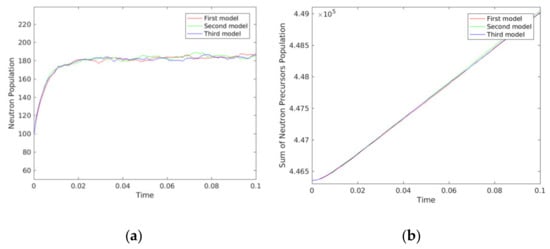
Figure 1.
Population for the second case study. (a) Neutron population. (b) Precursor population.
Table 3.
Population for the second case study at time t = 0.1 s.
Table 4.
Computational time for the second case study.
Table 3 shows instability (appearance of imaginary numbers) in the computation using the SPK model; however, Figure 1 and Table 3 show good agreement between the three SDE models, considering only the real parts for the SPK model. This instability is due to the computation of the square root in the diffusion term. Moreover, Table 4 shows the compatible efficiency of the LPK model and the SSPK model, with superiority over the SPK model.
6.3. Third Case
As a third test case, an actual prompt critical insertion in a nuclear reactor was considered with similar parameters as in the second test case [2]:
,
, ,
, , . The initial conditions were specified as
, and there was no external source, . In this experiment, the population’s mean and variance were estimated at time . For the SDE models, the time interval was divided into , and the number of trials was trials.
Figure 2 shows the evolution of the population’s mean (considering only the real parts for the SPK model) on the interval estimated using the three SDE models. Table 5 summarizes the mean and variance of the neutron and precursor populations at time . Table 6 shows the time consumed in seconds for the computations of the SDE models.
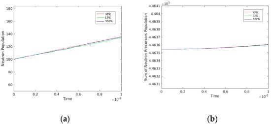
Figure 2.
Population for the third case study. (a) Neutron population. (b) Precursor population.
Table 5.
Population for the third case study at time t = 0.001 s.
Table 6.
Computational time for the third case study.
Table 5 shows instability in the computation using SPK model, due to the computation of the square root in the diffusion term; however, Figure 2 and Table 5 show a good agreement between the three SDE models, considering only the real parts for the SPK model. Moreover, Table 6 shows the compatible efficiency of the LPK model and the SSPK model, with superiority over the SPK model.
6.4. Fourth Case
As a fourth test case, a nonphysical nuclear reactor, similar to the first test case, was considered with the following parameters [2]: , , , , . The operation started at clear initial conditions, , and the external source was fixed at . In this experiment, we computed the mean and variance of the time needed of the reactor to reach the neutron population level . The step size was specified at , and the number of trials was trials.
Figure 3 shows the histogram of the required time for the neutron population to reach the density . Table 7 summarizes the mean and variance of the required time for the neutron population to reach the density . Table 8 shows the time consumed in seconds for the computation of the three SDE models.
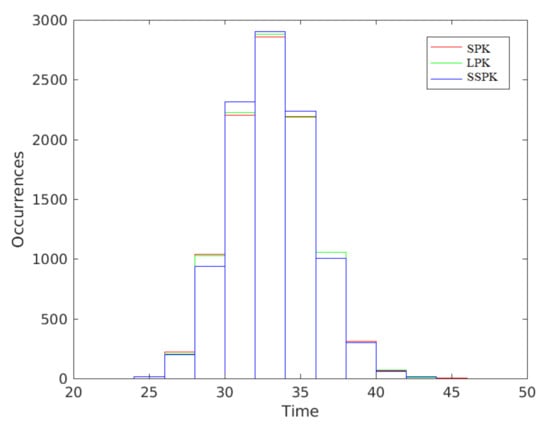
Figure 3.
Histogram of times for the fourth case study.
Table 7.
Mean and variance of times for the fourth case study.
Table 8.
Computational time for the fourth case study.
6.5. Fifth Case
As a fifth test case, we considered the Godiva reactor with the following parameters [2]: ,
, , , , . The operation started at clear initial conditions,
, and the external source was fixed at . In this experiment, we computed the mean and variance of the time needed for the reactor to reach the neutron population level . For the SDE models, the step size was specified at , and the number of trials was trials.
Figure 4 shows the histogram of the required time for the neutron population to reach the density . Table 9 summarizes the mean and variance of the required time for the neutron population to reach the density . Table 10 shows the time consumed in seconds for the computation of the three SDE models.
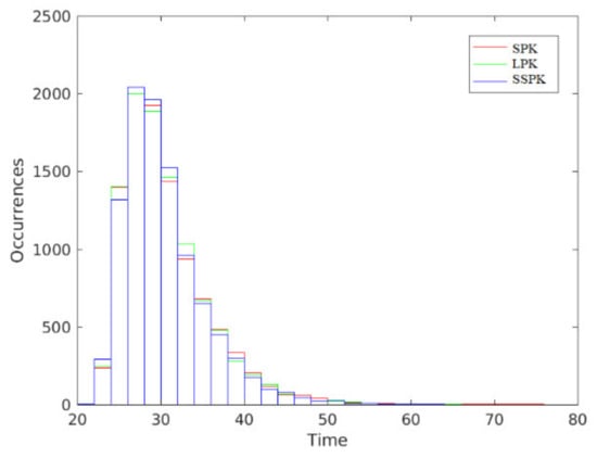
Figure 4.
Histogram of times for the fifth case study.
Table 9.
Mean and variance of times for the fifth case study.
Table 10.
Computational time for the fifth case study.
Figure 4 and Table 9 show a good agreement between the results of the three SDE models. Table 10 shows the compatible efficiency of the LPK model and the SSPK model, with superiority over the SPK model.
From the above results, we can deduce that the new LPK model combines the advantages, accuracy, and efficiency of the available models. The same technique can also be extended for other applications specially in biology and population dynamics. The model can be modified by considering the fractional derivatives instead of the integer-order derivatives. This will account for long-time and/or time-dependent correlations.
7. Conclusions
We reviewed two procedures to construct stochastic differential equation models and applied them to the point reactor. The first procedure follows the same steps as the procedure of constructing an ODE system, so we can benefit from its extensive literature. However, the second procedure has a simple method of construction. The critical benefit of the second procedure is that it does not require computations of the square root of the diffusion matrix, so it is more efficient and stable. This benefit loses its effect if the number of possible changes is much larger than the number of components, which is not the case with the point reactor. The newly developed LPK model, which is theoretically equivalent to the SPK model, achieved high performance compatible with the SSPK model and more stability than the SPK model. Another advantage is that the resultant model can be analyzed by spectral techniques such as Wiener-Hermite expansion. Many test cases are performed and the efficiency and accuracy of the newly developed LPK model are investigated.
Author Contributions
Conceptualization, A.E. and M.E.-B.; methodology, A.E. and M.E.-B.; software, A.E.; validation, M.E.-B., A.A.-J. and S.A.-Q.; formal analysis, M.E.-B.; investigation, M.E.-B., A.A.-J. and S.A.-Q.; resources, A.A.-J. and S.A.-Q.; writing—original draft preparation, A.E.; writing—review and editing, M.E.-B., A.A.-J. and S.A.-Q.; visualization, A.E. and M.E.-B.; supervision M.E.-B. and A.A.-J.; project administration, A.A.-J. All authors have read and agreed to the published version of the manuscript.
Funding
This research received no external funding.
Informed Consent Statement
Not applicable.
Data Availability Statement
Not applicable.
Conflicts of Interest
The authors declare no conflict of interest.
References
- Hetrick, D.L. Dynamics of Nuclear Reactors; University of Chicago Press: Chicago, IL, USA, 1971; pp. 1–542. [Google Scholar]
- Hayes, J.; Allen, E. Stochastic point-kinetics equations in nuclear reactor dynamics. Ann. Nucl. Energy 2005, 32, 572–587. [Google Scholar] [CrossRef]
- Ayyoubzadeh, S.M.; Vosoughi, N. An alternative stochastic formulation for the point reactor. Ann. Nucl. Energy 2014, 63, 691–695. [Google Scholar] [CrossRef]
- Gillespie, D.T. Approximate accelerated stochastic simulation of chemically reacting systems. J. Chem. Phys. 2001, 115, 1716–1733. [Google Scholar] [CrossRef]
- El-Beltagy, M.; Noor, A. Analysis of the stochastic point reactor using Wiener-Hermite expansion. Ann. Nucl. Energy 2019, 134, 250–257. [Google Scholar] [CrossRef]
- Alaskary, S.; El-Beltagy, M. Uncertainty Quantification Spectral Technique for the Stochastic Point Reactor with Random Parameters. Energies 2020, 13, 1297. [Google Scholar] [CrossRef]
- Ha, P.N.V.; Kim, J.-K. Further evaluation of a stochastic model applied to monoenergetic space-time nuclear reactor kinetics. Nucl. Eng. Technol. 2011, 43, 523–530. [Google Scholar] [CrossRef]
- Ha, P.N.V.; Kim, J.K. A stochastic approach to monoenergetic space-time nuclear reactor kinetics. J. Nucl. Sci. Technol. 2010, 47, 705–711. [Google Scholar] [CrossRef]
- Kinard, M.; Allen, E. Efficient numerical solution of the point kinetics equations in nuclear reactor dynamics. Ann. Nucl. Energy 2004, 31, 1039–1051. [Google Scholar] [CrossRef]
- Allen, E.J.; Allen, L.J.S.; Arciniega, A.; Greenwood, P.E. Construction of Equivalent Stochastic Differential Equation Models. Stoch. Anal. Appl. 2008, 26, 274–297. [Google Scholar] [CrossRef]
- Allen, E.J. Modeling with Itx Stochastic Differential Equations, 1st ed.; Springer Netherlands: Dordrecht, The Netherlands, 2007; Volume 1, pp. 1–228. [Google Scholar]
- Allen, L.J.S. An Introduction to Stochastic Processes with Applications to Biology, 2nd ed.; CRC Press: Boca Raton, FL, USA, 2010; pp. 1–496. [Google Scholar]
- Gillespie, D.T. The chemical Langevin equation. J. Chem. Phys. 2000, 113, 297–306. [Google Scholar] [CrossRef]
Publisher’s Note: MDPI stays neutral with regard to jurisdictional claims in published maps and institutional affiliations. |
© 2021 by the authors. Licensee MDPI, Basel, Switzerland. This article is an open access article distributed under the terms and conditions of the Creative Commons Attribution (CC BY) license (http://creativecommons.org/licenses/by/4.0/).