A Carbon Price Prediction Model Based on the Secondary Decomposition Algorithm and Influencing Factors

Abstract

Carbon emission reduction is now a global issue, and the prediction of carbon trading market prices is an important means of reducing emissions. This paper innovatively proposes a second decomposition carbon price prediction model based on the nuclear extreme learning machine optimized by the Sparrow search algorithm and considers the structural and nonstructural influencing factors in the model. Firstly, empirical mode decomposition (EMD) is used to decompose the carbon price data and variational mode decomposition (VMD) is used to decompose Intrinsic Mode Function 1 (IMF1), and the decomposition of carbon prices is used as part of the input of the prediction model. Then, a maximum correlation minimum redundancy algorithm (mRMR) is used to preprocess the structural and nonstructural factors as another part of the input of the prediction model. After the Sparrow search algorithm (SSA) optimizes the relevant parameters of Extreme Learning Machine with Kernel (KELM), the model is used for prediction. Finally, in the empirical study, this paper selects two typical carbon trading markets in China for analysis. In the Guangdong and Hubei markets, the EMD-VMD-SSA-KELM model is superior to other models. It shows that this model has good robustness and validity.

1. Introduction

Agriculture, fisheries, and animal husbandry are the main contributors to the development of the global economy. The increase in temperature caused by carbon dioxide emissions has a huge impact on them. Because global warming has led to reduced fishery production and threatened food security, this will affect the development of the global economy and the environment for human survival [1]. Global warming has aggravated the frequency of river drought and caused serious damage to the ecosystem [2]. In summary, carbon dioxide emissions have had an important impact on the human living environment, natural ecosystems, and the development of the global economy. Therefore, we should reduce carbon emissions as our urgent problem.

To reduce carbon emissions worldwide, the international community has adopted carbon dioxide emissions trading rights as an important economic measure to deal with global warming, which is very important for the global promotion of carbon emissions reduction. The European Union Emissions Trading Scheme (EU ETS) is an important mechanism to deal with carbon emissions. The EU ETS is the first, largest, and most prominent carbon emission regulatory system in European countries. The EU Emissions Trading Program has established European Union Permits (EUAs), and emitters have a certain number of EU permits, and emitters can freely trade EUAs. In this way, emission reduction targets can be achieved at the lowest cost, especially it is very effective in reducing industrial carbon emissions [3]. EU ETS has an important impact on the performance of enterprises. 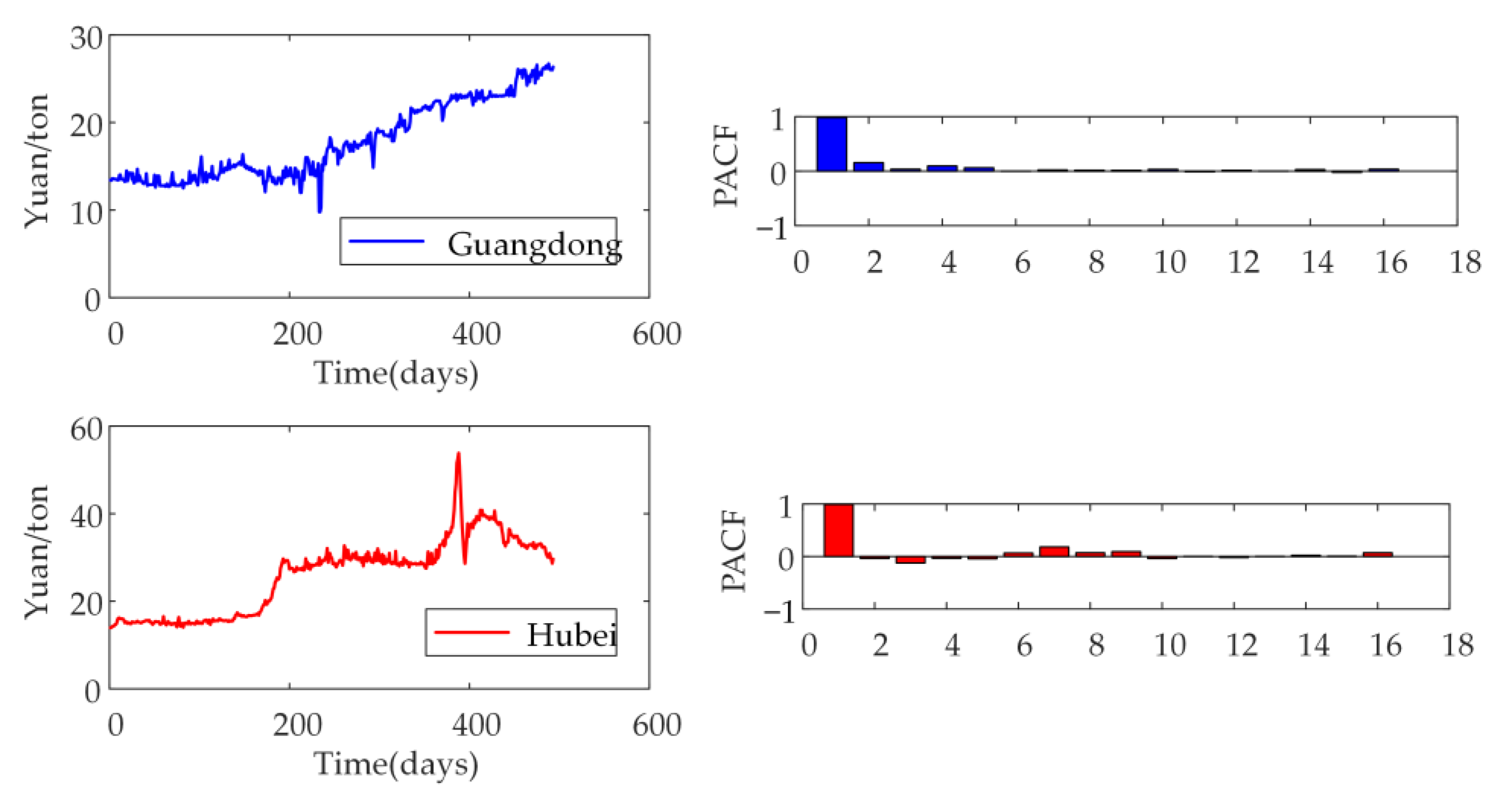The performance of enterprises with free carbon emission allowances is significantly better than that of enterprises without free carbon emission allowances [4]. At the same time, EU ETS is also a good benchmark for China. China is becoming the world’s largest carbon emitter. Since 2011, China has launched carbon trading pilot projects in 8 provinces and cities including Beijing, Tianjin, Shanghai, Chongqing, Hubei, Guangdong, Shenzhen, and Fujian. At present, China’s carbon market is making every effort to promote the construction of the carbon market, and it is expected that a unified national carbon market will be formed around 2020 [5]. According to this plan, China will have about 3 billion tons of carbon emissions trading. This scale will exceed the EU.

There are currently three main carbon price predictions. The first is a quantitative statistical model. The second is a neural network model. The third is a hybrid model.

The first is the quantitative statistical model. They are autoregressive integral moving average (ARIMA) model [6], Generalized Auto Regressive Conditional Heteroskedasticity (GARCH) model [7], and ARIMA-GARCH model [8]. However, due to the high complexity and nonlinearity of carbon prices, the prediction results of statistical models are often not ideal. With the development of neural networks and deep learning, the second is the neural network model prediction. The backpropagation neural network (BP) model [9], the least square support vector machine method (LSSVM) model [10], and the artificial neural network (MLP) model [11] are the other models.

Because carbon prices are complex and very unstable, a single model cannot fully capture them. However, with the popularization and application of digital signal technology, digital signal decomposition technology has also been applied to the field of carbon price prediction. The third type is the neural network hybrid model [12]. Zhu compared the model combining empirical mode decomposition (EMD) and genetic algorithm optimization (GA) artificial neural network (ANN) with the GA-ANN model and proved the effectiveness of EMD decomposition [13]. Li et al. proposed an EMD-GARCH model [14]. Zhu et al. used EMD and particle swarm optimization (PSO) optimized LSSVM model to predict carbon prices [15]. Sun et al. used an extreme learning machine (ELM) optimized by EMD and PSO to predict carbon prices [16]. Sun et al. used variational modal decomposition (VMD) and Spike Neural Network (SNN) models to predict carbon prices [17]. Zhu et al. proposed VMD, model reconstruction (MR), and optimal combination forecasting model (CFM) combined model to predict carbon prices [18]. Liu et al. proposed that EMD can reduce the nonlinearity and complexity of carbon price time series, but there is still room for improvement [19]. In terms of wind speed prediction, compared with the primary decomposition prediction model, the performance of the secondary decomposition prediction model is better [20,21,22]. Secondary decomposition is also used for carbon price prediction. Sun et al. proposed an EMD-VMD model to predict carbon prices, which verified that the EMD-VMD model is more effective than the EMD model [23,24].

In addition to considering the time series of carbon prices, carbon price prediction also needs to consider influencing factors. Byun et al. verified that carbon prices are also related to Brent crude oil, coal, natural gas, and electricity [25]. Zhao et al. verified that coal is the best factor for carbon price prediction [26]. Dutta used the Crude Oil Volatility Index (OVX) to study the impact of oil market uncertainty on emission price fluctuations [27]. Sun et al. used a one-time decomposition algorithm combined with influencing factor models to predict carbon prices [28,29].

In summary, the neural network hybrid forecasting model is a trend. Influencing factors are very important for carbon price prediction. EMD-VMD is a good decomposition method. Since the ELM model randomly sets the hidden layer parameters and brings about the problem of poor stability, the kernel function mapping replaces the random mapping of the hidden layer, avoiding this problem and improving the robustness of the model. Kernel Extreme Learning Machine (KELM) is a good neural network model. However, KELM also has the problem of the influence of kernel parameter settings [30]. This paper uses the latest sparrow search algorithm (SSA) to optimize the kernel parameters of KELM and obtain the optimal model. Finally, this paper proposes the EMD-VMD-SSA-KELM model. This model may have three main contributions. The first is that there is few literature on carbon price prediction models based on the secondary decomposition algorithm (Enriched models in this area). The second is that there are still gaps in the literature on the carbon price prediction model based on the combination of the secondary decomposition algorithm and multiple influencing factors. This model fills the gap in this area. The third document about KELM’s carbon price prediction model is relatively small. This paper proposed the latest SSA-KLEM model to predict carbon prices, which enriches the models in this area.

Introduce the rest of this article. The second part is the methods and models, including EMD, VMD, KELM, SSA, and the EMD-VMD-SSA-KELM model framework proposed in this paper. The third part is the collection of data including carbon price, structural influencing factors, and nonstructural influencing factors (the primary and secondary decomposition of carbon prices). The fourth part is model input and parameter setting. The fifth part is the prediction result and error analysis. The sixth part is the additional forecast, and the seventh part is the conclusion.

2. Method

2.1. Empirical Mode Decomposition

EMD is a signal decomposition algorithm [31]. EMD decomposition is to decompose a signal $f\left(t\right)$ into Intrinsic Mode Functions (IMFs) and a residual. The following prerequisites must be met by every IMF: in the whole data, the amount of local extreme points and zero points must be the same or at most one difference. At any point in the data, the sum value of the upper envelope and the lower envelope must be zero.

The decomposition principle of EMD is as below:

Step 1: find out all the local maximum and minimum points in the signal, and then combine each extreme point to construct the upper envelope and lower envelope by the curve fitting method, so that the original signal is Enveloped by the upper and lower envelopes.

Step 2: the mean curve $m\left(t\right)$ can be constructed from the upper and lower envelope lines, and then the original signal $f\left(t\right)$ is subtracted from the mean curve, so the obtained $H\left(t\right)$ is the IMF.

Step 3: since the IMF obtained in the first and second steps usually does not meet the two conditions of the IMF, the first and second steps must be repeated until the $SD$ (screening threshold, generally 0.2~0.3) is less than the threshold. It stops when the limit is reached so that the first $H\left(t\right)$ that meets the condition is the first IMF. How to find $SD$:

$$SD={\displaystyle \sum }_{t=0}^r\frac{{\left|H_{K-1}\left(t\right)-H_k\left(t\right)\right|}^2}{{{\displaystyle \sum }}_{t=0}^T{H}_{K-1}{}^2\left(t\right)}$$

(1)

Step 4: Residual:

$$r\left(t\right)=f\left(t\right)-H\left(t\right)$$

(2)

Repeat the first, second, and third steps until $r\left(t\right)$ meets the preset conditions.

2.2. Variational Mode Decomposition

VMD is an adaptive, completely non-recursive modal change and signal processing method [32]. This technique has the advantage of being able to determine the number of modal decompositions. It can achieve the best center frequency and limited bandwidth, can achieve the effective separation of the IMF, signal frequency domain division, and then obtain the effective decomposition component of a given signal. First, construct the variational problem. Assuming that the original signal $f$ is decomposed into $k$ components, each modal component must have a center frequency and a limited bandwidth, and the sum of the estimated bandwidth of each model is the smallest. The sum of all modal components is equivalent to the original signal as a constraint condition. The corresponding constraint variational expression is

$$\{\begin{array}{c}\begin{array}{c}min\\ \{u_k\}\left\{{\omega }_k\right\}\end{array}\left\{{\displaystyle \sum }_k\Vert {\partial }_t\left[\left(\sigma \left(t\right)+\frac{j}{\pi t}\right)\ast u_k\left(t\right)\right]e^{-j{w}_{k}t}{\Vert }_2^2\right\}\\ s.t.{\displaystyle \sum }_{k=1}^K{u}_k=f\end{array}$$

(3)

In the Formula (3): $K$ is the number of decomposed modes, $\left\{{\mu }_k\right\},\left\{{\omega }_k\right\}$ correspond to the K-th component and its central frequency, and $\delta \left(t\right)$ is the Dirac fir tree. * is the convolution operator.

Then, by solving Equation (3) and introducing Lagrange multiplication operator $\lambda$, the constrained variational problem is transformed into an unconstrained variational problem, and the augmented Lagrange expression is obtained.

$$L\left(\left\{u_k\right\},\left\{{\omega }_k\right\},\lambda \right)=\alpha {\displaystyle \sum }_k\Vert {\partial }_t\left[\left(\sigma \left(t\right)+\frac{j}{\pi t}\right)\ast u_k\left(t\right)\right]e^{-j{w}_{k}t}{\Vert }_2^2+\Vert f\left(t\right)-{\displaystyle \sum }_k{u}_k{\left(t\right)\Vert }_2^2+\langle \lambda \left(t\right),f\left(t\right)-{\displaystyle \sum }_k{u}_k\left(t\right)\rangle$$

(4)

In Formula (4): $\alpha$ is the secondary penalty factor, and its function is to reduce the interference of Gaussian noise. Using the Alternating Direction Multiplier (ADMM) iterative algorithm combined with Parseval, Fourier equidistant transformation, optimize the modal components and center frequency, and search for the saddle point of the augmented Lagrange function, alternately optimize $u_k,{\omega }_k,$ and $\lambda$ after iteration. These formulas are as follows.

$${\widehat{u}}_n^{k+1}\left(\omega \right)\leftarrow \frac{\widehat{f}\left(\omega \right)-{{\displaystyle \sum }}_{i\ne k}{\widehat{u}}_i\left(\omega \right)+\widehat{\lambda }\left(\omega \right)/2}{1+2\alpha {\left(\omega -{\omega }_k\right)}^2}$$

(5)

$${\omega }_k^{n+1}\leftarrow \frac{{{\displaystyle \int }}_0^{\infty }\omega {\left|{\widehat{u}}_n^{k+1}\left(\omega \right)\right|}^{2}d\omega }{{{\displaystyle \int }}_0^{\infty }{\left|{\widehat{u}}_n^{k+1}\left(\omega \right)\right|}^{2}d\omega }$$

(6)

$${\widehat{\lambda }}^{n+1}\left(\omega \right)\leftarrow {\widehat{\lambda }}^n\left(\omega \right)+\gamma (\widehat{f}\left(\omega -{\displaystyle \sum }_k{\widehat{u}}_k^{n+1}\left(\omega \right)\right)$$

(7)

In the formula: $\gamma$ is the noise tolerance, which satisfies the fidelity requirement of signal decomposition, ${\widehat{u}}_n^{k+1}\left(\omega \right),{\widehat{u}}_i\left(\omega \right)$, $\widehat{f}\left(\omega \right)$, $\widehat{\lambda }\left(\omega \right)$ correspond to $u_n^{k+1}\left(t\right)$,$u_i\left(t\right)$,$f\left(t\right)$ and Fourier transforms of $\lambda \left(t\right)$, respectively.

The main iteration requirements of VMD are as follows:

1:

Initialize $\widehat{u}{ }_k^1 ,\omega { }_k^1,{\lambda }^1$ and the maximum number of iterations N, $0\leftarrow n$.

2:

Use Formulas (5) and (6) to update ${\widehat{u}}_k$ and ${\omega }_k$.

3:

Use Formula (7) to update $\widehat{\lambda }$.

4:

Accuracy convergence judgment basis $\epsilon >0$, if not satisfied ${\displaystyle \sum }_k\Vert {\widehat{u}}_k^{n+1}-{\widehat{u}}_k^n{\Vert }_2^2<\epsilon and n<\mathrm{N}$, return to the second step, otherwise complete the iteration and output the final ${\widehat{\mu }}_k$ and ${\omega }_k$.

2.3. Sparrow Search Algorithm

SSA is a new swarm intelligence optimization algorithm [33]. Its bionic principles are as follows:

The sparrow foraging process can be abstracted as a discoverer–adder model, and a reconnaissance early warning mechanism is added. The discoverer itself is highly adaptable and has a wide search range, guiding the population to search and forage. To obtain better fitness, the joiner follows the discoverer for food. At the same time, to increase their predation rate, some joiners will monitor the discoverer to fight for food or forage around them. When the entire population faces the threat of predators or realizes the danger, it will immediately carry out anti-predation behavior.

In SSA, the solution to the optimization problem is obtained by simulating the foraging process of sparrows. Assuming that there are $N$ sparrows in a D-dimensional search space, the position of the i-th sparrow in the D-dimensional search space is $X_I=\left[x_{il},\dots ,x_{id},\dots ,x_{iD}\right]$ where $i=1,2,\dots ,N$, $x_{id}$ represents the position of the i-th sparrow in the d-th dimension.

Discoverers generally account for 10% to 20% of the population. The position update formula is as follows:

$$x_{id}^{t+1}=\{\begin{array}{c}{x}_{id}^t\ast exp\left(\frac{-i}{\alpha \ast T}\right),R_2<ST\\ x_{id}^t+Q\ast L,R_2\ge ST\end{array}$$

(8)

In Formula (8): t represents the current number of iterations. $T$ represents the maximum number of iterations. $\alpha$ is a uniform random number between $\left[0,1\right]$.$Q$ is a random digit that submits to a standard normal distribution. $L$ represents a size of 1xd, with all elements $A$ matrix of 1. $R_2\in \left[0,1\right]$ is the warning value. $ST\in \left[0.5,1\right]$ is a safe value. When $R_2<ST$, the population does not find the presence of predators or other dangers, the search environment is safe, and the discoverer can search extensively to guide the population to obtain higher fitness. When $R_2\ge ST$, the sparrows are detected and the predators are found. The danger signal was immediately released, and the population immediately performed anti-predation behavior, adjusted the search strategy, and quickly moved closer to the safe area.

Except for the discoverer, the remaining sparrows are all joiners and update their positions according to the following formula:

$$x_{id}^{t+1}=\{\begin{array}{c}Q\ast exp\left(\frac{x{w}_d^t-x_{id}^t}{i^2}\right),i>\frac{n}{2}\\ x{b}_d^{t+1}+\frac{1}{D}{\displaystyle \sum }_{d=1}^D\left(rand\left\{-1,1\right\}\ast \left|x_{id}^t-x{b}_d^{t+1}\right|\right),i\le \frac{n}{2}\end{array}$$

(9)

In the Formula (9): $x{w}_d^t$ is the worst position of the sparrow in the d dimension at the t-th iteration of the population. $x{b}_d^{t+1}$ represents the optimal position of the sparrow in the d dimension at the (t+1)-th iteration of the population position. When $I>\frac{n}{2}$, it indicates that the i-th joiner has no food, is hungry, and has low adaptability. To obtain higher energy, he needs to fly to other places for food. When $I\le \frac{n}{2}$, the i-th joiner will randomly find a location near the current optimal position $x_b$ for foraging.

Sparrows for reconnaissance and early warning generally account for 10% to 20% of the population. The location is updated as follows:

$$x_{id}^{t+1}=\{\begin{array}{c}x{b}_d^t+\beta \left(x_{id}^t-x{b}_d^t\right),f_i\ne f_g\\ x_d^{t+1}+K\left(\frac{x_{id}^t-x{w}_d^t}{\left|f_i-f_w\right|+e}\right),f_i=f_g\end{array}$$

(10)

In the Formula (10): $\beta$ is the step control parameter, which is a random digit subject to $N\left(0,1\right)$. $K$ is a random number between $\left[-1,1\right]$, indicating the direction of the sparrow’s movement, which is also a step Long control parameter, e is a minimal constant to avoid the situation where the denominator is 0. $f_i$ represents the fitness value of the i-th sparrow, $f_g$ and $f_w$ are the optimal and worst fitness values of the current sparrow population, respectively. When $f_i\ne f_g$, it makes known that the sparrow is at the margin of the whole population and is easily attacked by predators. When $f_i=f_g$, it indicates that the sparrow is in the center of the whole population because it is aware of the threat of predators to avoid being attacked by predators and get close to other sparrows in time to adjust the search strategy.

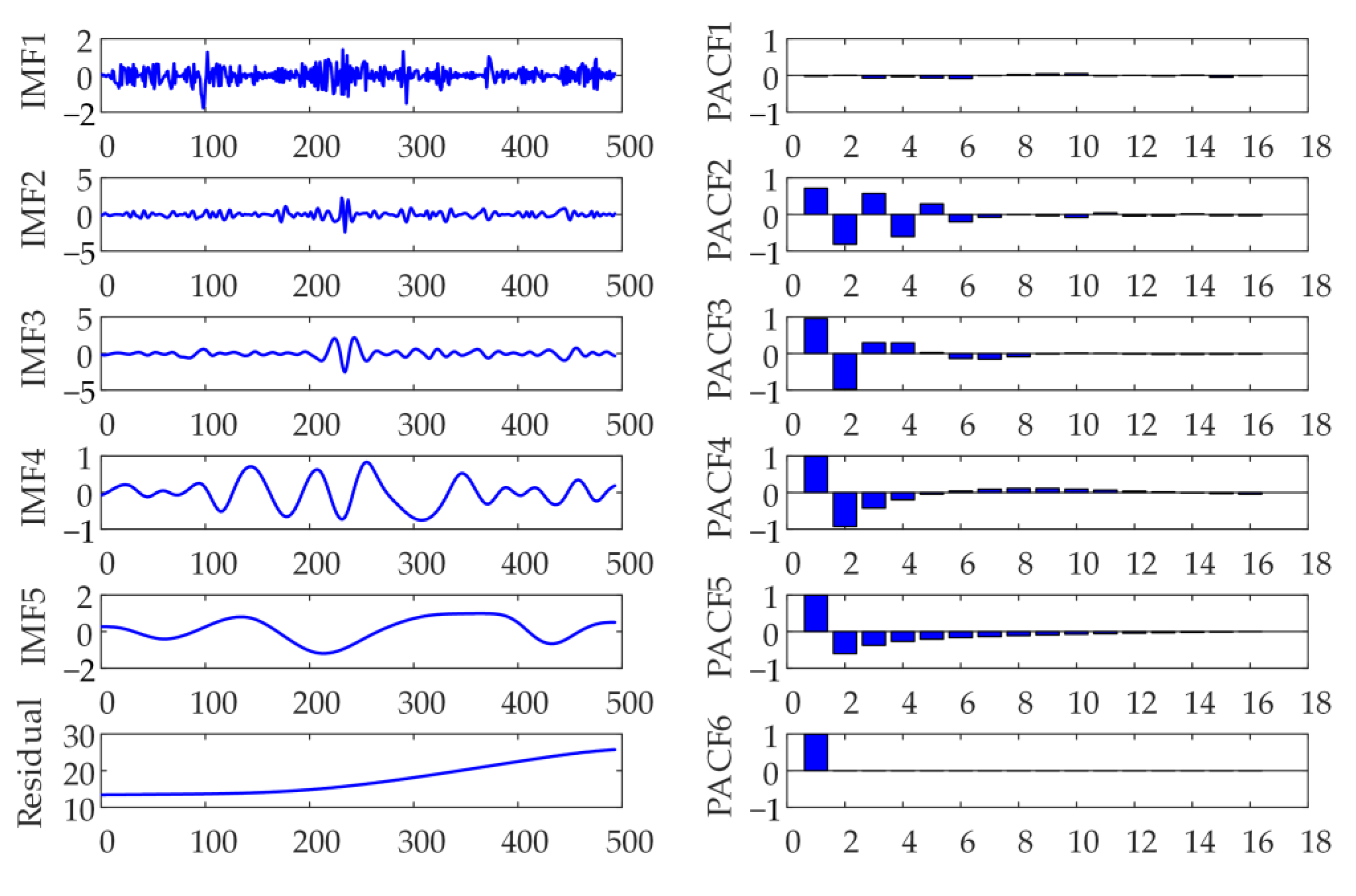
2.4. Partial Autocorrelation Function

The relationship between time series and their lags is given. Based on the lag order, the input and output variables of the neural network are determined. Given the time series $x_t$ with ${\varphi }_{kj}$ representing the autoregressive equation of $j$ and $k$ order regression coefficients, the k order autoregressive model is expressed as

$$x_t={\varphi }_{k1}{x}_{t-1}+{\varphi }_{k2}{x}_{t-2}+\dots +{\varphi }_{kk}{x}_{t-k}+{\mu }_t$$

(11)

2.5. Maximum Correlation Minimum Redundancy Algorithm

mRMR is to find the most relevant feature in the original feature set, but the least correlation with each other, and to use mutual information to express the correlation [34]. The mutual information between the two variables $X$ and $Y$ is:

$$I\left(X,Y\right)=\iint p\left(X,Y\right)\log \frac{p\left(X,Y\right)}{p\left(X\right)p\left(Y\right)}dXdY$$

(12)

The Sub-Formulas $p\left(X\right)$, $p\left(Y\right)$ are frequency functions, and $p\left(X, Y\right)$ are joint frequency functions.

Based on mutual information, the core expression of the algorithm is

$$\{\begin{array}{c}max D\left(S,p\right)\\ D=\frac{1}{n}{\displaystyle {\displaystyle \sum }_{i=1}^n}I\left(x,p\right)\end{array}$$

(13)

$$\{\begin{array}{c}minR\left(S\right)\\ R=\frac{1}{C_n^2}{\displaystyle {\displaystyle \sum }_{i=1}^{n-1}}{\displaystyle {\displaystyle \sum }_{j=i+1}^n}I\left(x_i,x_j\right)\end{array}$$

(14)

In the formula, Formula (13) represents the maximum correlation, Formula (14) represents the minimum redundancy. $S$ is the feature subset. n shows the number of features. $I\left(x,p\right)$ shows the mutual information between the feature and the target feature. $P$ represents the target feature. $I\left(x_i,x_j\right)$ represents the mutual information between the features.

Generally, through the wig integration Formulas (13) and (14), the final maximum correlation and minimum redundancy judgment conditions are obtained:

$$\{\begin{array}{c}max\varphi \left(D,R\right)\\ \varphi \left(D,R\right)=D-R\end{array}$$

(15)

2.6. Extreme Learning Machine with Kernel

KELM is an extension of ELM by Huang et al. [35]. The kernel function mapping is used to replace the random mapping of the hidden layer, which avoids the problem of poor stability caused by randomly given hidden layer parameters by ELM, and improves the robustness of the model. Because of its fast calculation speed and strong generalization ability, KELM’s basic principles are as follows:

Assuming that the number of hidden layer nodes is L, the hidden layer output function is $h\left(x\right)=\left[h_1\left(x\right),\dots ,h_l\left(x\right)\right]$, the hidden layer output weight $\beta =\left[{\beta }_1,\dots ,{\beta }_l\right]$, training sample set $\left\{\left(x_i,t_i)|x_i\in R^d,t_i\in R^m,i=1,\dots ,l\right)\right\},$ the ELM model can be shown as:

$$f\left(x\right)={{\displaystyle \sum }}_{i=1}^L{\beta }_i{h}_i\left(x\right)=h\left(x\right)\beta$$

(16)

The goal of ELM is to minimize the training error and the output weight $\beta$ of the hidden layer. Based on the principle of minimum structural risk, a quadratic programming problem is constructed as follows:

$$\{\begin{array}{c}\min L_P=\frac{1}{2}\Vert {\beta }^2\Vert +\frac{C}{2}{\displaystyle {\displaystyle \sum }_{I=1}^L}\Vert {\xi }_i\Vert {}^2\\ s.t.h\left(x_i\right)\beta =t_i^T-{\xi }_i^T,i=1,\dots ,l\end{array}$$

(17)

In the formula, C is the penalty factor;${\xi }_i$ is the i-th error variable.

Introducing the Lagrange multiplier ${\alpha }_i$, the quadratic programming problem of Equation (17) is transformed into:

$$L=\frac{1}{2}\Vert {\beta }^2\Vert +\frac{C}{2}{\displaystyle \sum }_{I=1}^L\Vert {\xi }_i\Vert {}^2-{\displaystyle \sum }_{i=1}^l{\alpha }_i\ast \left(h\left(x_i\right)\beta -t_i^T+{\xi }_i^T\right)$$

(18)

According to the KKT condition, the derivatives of $\beta , {\xi }_i$, and ${\alpha }_i$ are obtained, respectively. Finally, get the output weight of the ELM model:

$$\beta =H^T{\left(\frac{I}{C}+H{H}^T\right)}^{-1}T$$

(19)

In the Formula (19): $H$ is the hidden layer matrix, $T$ is the target value matrix, $I$ is the identity matrix.

To improve the prediction accuracy and stability of the model, the kernel matrix is introduced to replace the hidden layer matrix $H$ of ELM, and the training samples are mapped to high-dimensional space through the kernel function. Define the kernel matrix as ${\mathsf{\Omega }}_{ELM}$, and the elements ${\mathsf{\Omega }}_{ELM}\left(i,j\right)$, construct the KELM model as follows:

$$\{\begin{array}{c}{\mathsf{\Omega }}_{ELM,}=H{H}^T\\ {\mathsf{\Omega }}_{ELM}\left(i,j\right)=K\left(x_i,x_j\right)\end{array}$$

(20)

$$f\left(x\right)=h\left(x\right)\beta =H^T{\left(\frac{I}{C}+H{H}^T\right)}^{-1}T=\left[\begin{array}{c}K\left(x,x\right)\\ \dots \\ K\left(x,x\right)\end{array}\right]{\left(\frac{I}{C}+{\mathsf{\Omega }}_{ELM,}\right)}^{-1}T$$

(21)

In the Formula (20), $K\left(x_i,x_j\right)$ usually chooses radial basis kernel function and linear kernel function, and the expressions are shown in Formulas (22) and (23):

$$K\left(x_i,x_j\right)=exp\left(\frac{-\Vert x_{i-}{x}_j\Vert }{{\sigma }^2}\right)$$

(22)

In the Formula (22), ${\sigma }^2$ is the width parameter of the kernel function.

$$K\left(x_i,x_j\right)=x_i{x}_j{}^T$$

(23)

Although the introduction of the kernel function increases the stability of the prediction model, $C$ and ${\sigma }^2$ affect the two important parameters of the KELM prediction accuracy during the training process. If $C$ is too small, a larger training error will occur, and if $C$ is too large, overfitting will occur. Moreover, ${\sigma }^2$ affects the generalization performance of the model.

2.7. The Proposed Model

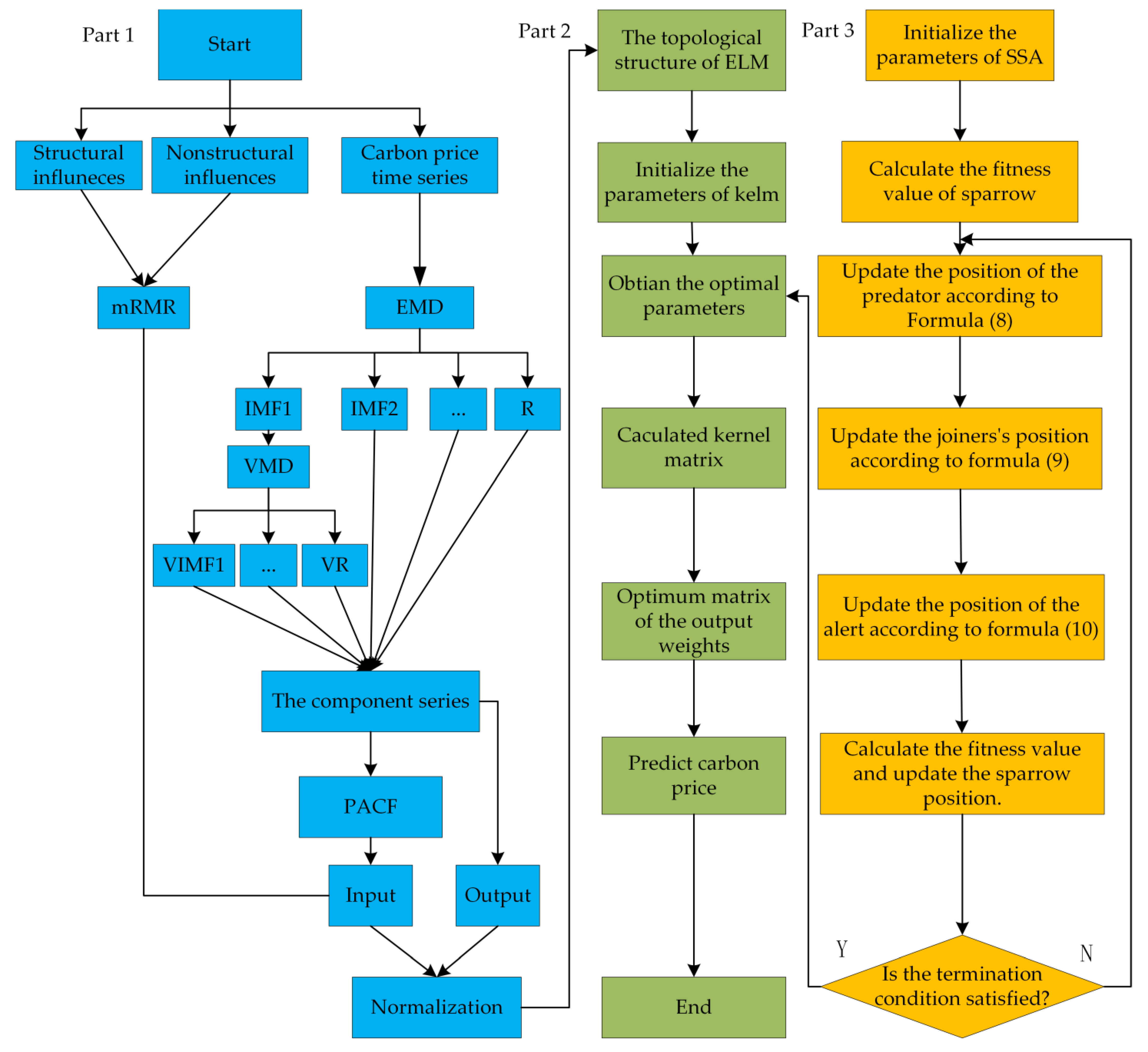
This structural model is based on a new carbon price prediction model proposed by data preprocessing technology, structural influencing factors, nonstructural influencing factors, feature selection technology, sparrow search algorithm, and secondary decomposition algorithm. Figure 1 shows the flow chart of the EMD-VMD-SSA-KLEM model.

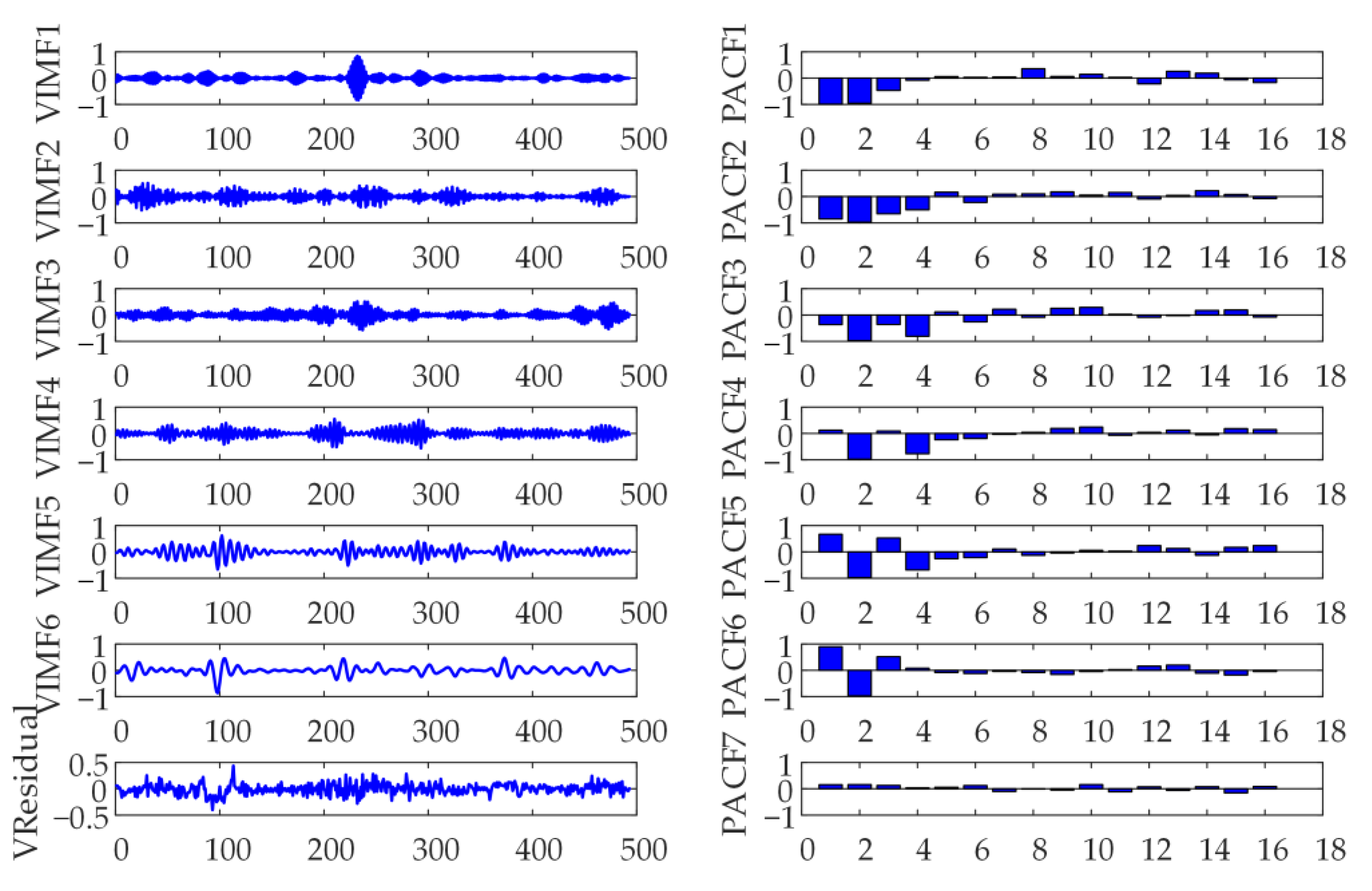
(1)

Part 1 is the flow chart of carbon price prediction. EMD is used to decompose the initial carbon price to obtain a decomposed IMF. Then, use variational modal decomposition to decompose IMF1 to get the VIMF of secondary decomposition. VIMF is the inherent mode function generated by VMD decomposition of IMF1.This is the output of the model.

(2)

Partial autocorrelation function (PACF) is used to select the features of the decomposed components, and then as part of the input of the model. Considering the structural and nonstructural factors, mRMR is used to reduce the dimension of the influencing factors, and the best feature of the influencing input is selected as the other part of the input of the model.

(3)

Part 2 is the flow chart of the KELM model. Part 3 is the SSA flow chart. Since in the KELM algorithm, system performance is mainly affected by the selection of γ and C, cross-validation is generally used for parameter confirmation. To avoid the influence caused by parameter selection, on this basis, the searchability of the sparrow search algorithm is combined with the fast-learning ability of KELM, and the γ and C of the model are optimized and evolved to obtain the optimal SSA-KELM prediction model.

(4)

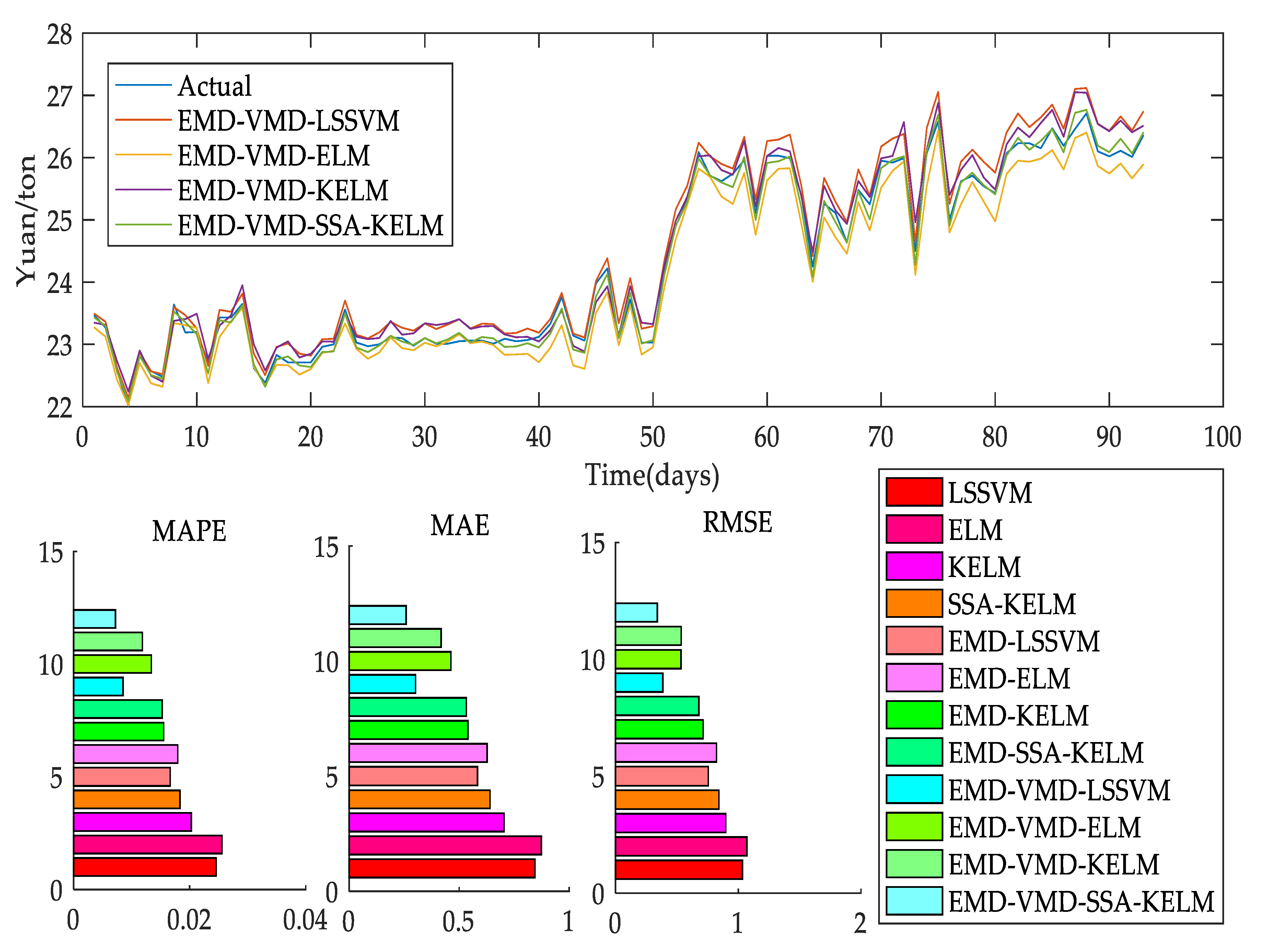
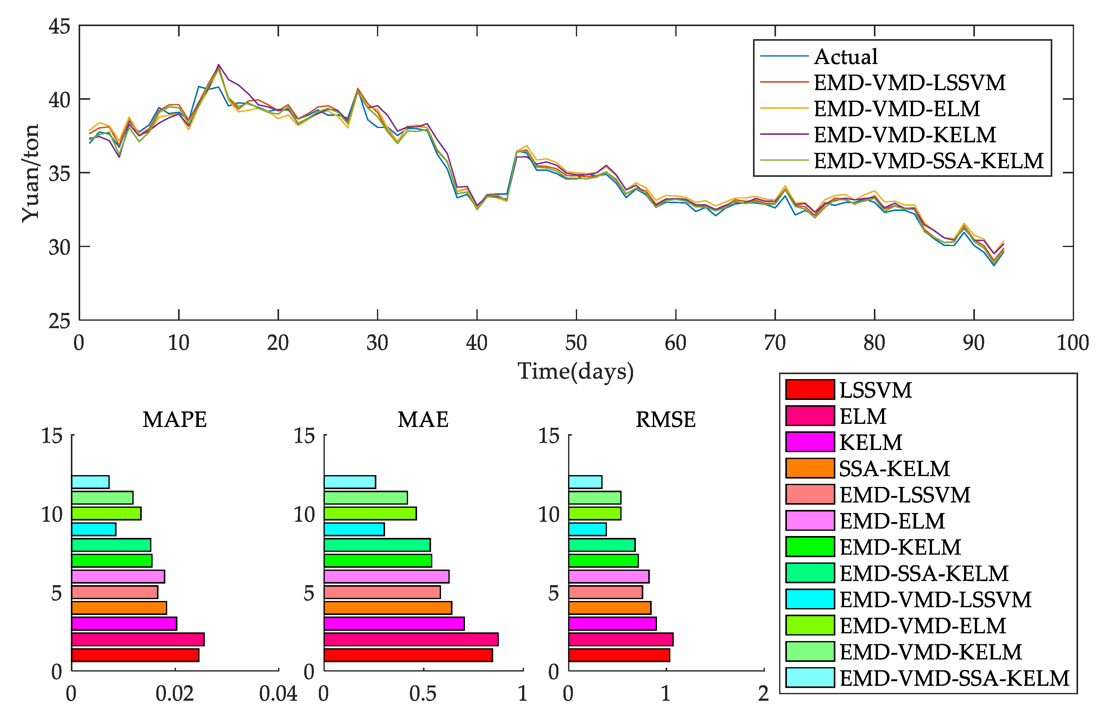
Establish undecomposed models, EMD models, EMD-VMD models, and other multiple models as Figure 2 to verify the superiority of the EMD-VMD-SSA-KELM model.

3. Data Preprocessing

3.1. Data Collection

China is one of the largest carbon emitters in the world and is facing increasing pressure to reduce emissions. Carbon price forecasting is of great significance to grasp the dynamic changes of prices in China’s carbon trading market. Therefore, this paper studies the daily carbon price data in China to prove the robustness and accuracy of the prediction model framework proposed in this paper. According to the carbon market investment index recommendation of the China Carbon Emissions Trading Network, we have selected the first two typical carbon trading markets, Guangdong and Hubei, respectively, and the daily carbon prices of these two markets are used as the main research data of this article. These data come from China Carbon Emissions Trading Network. Besides, we consider that carbon prices may be affected by a variety of factors and have complex features such as uncertainty. Therefore, the various influencing factors we consider have an important impact on carbon price forecasts. The factors we consider include the structural influencing factors on the supply side and the demand side, and the nonstructural influencing factors on the Baidu index.

3.1.1. Carbon Price

The carbon price selected in this paper takes into account the differences in public holidays and trading hours at home and abroad, as well as the impact of variable missing values. This paper selects public time. The Guangdong dataset selects the carbon price from 31 October 2017 to 4 November 2019, and the Hubei dataset selects the carbon price from 31 October 2017 to 7 November 2019 and their training datasets. There are a total of 493 data. Generally, the ratio of the experimental training set to the testing set is about 8:2. It is shown in

Table 1. The carbon price in Guangdong and Hubei.

Market	Size	Training Set	Testing Set	Training Set Data	Test Set Data	Date
Guangdong	493	400	93	2017/10/31–2019/6/18	2019/6/19–2019/11/4	2017/10/31–2019/11/4
Hubei	493	400	93	2017//10/31–2019/6/21	2019/6/22–2019/11/7	2017/10/31–2019/11/7

.

3.1.2. Structural Influence Factors

Domestic carbon prices are affected by supply and demand factors. First, carbon emission allowances are the largest supply-side influencing factor of the carbon market transaction price. At the same time, the EU carbon emission allowance (EUA) price is the benchmark of the global carbon trading market, which has an important impact on carbon emission allowances. Taking into account the market linkage, this paper selects the EUA Futures and Certified Emission Reduction (CER) Futures carbon prices as the international carbon prices. Then, the use of fossil energy is the main reason for carbon emissions. The price of coal is the settlement price of Rotterdam coal futures, the price of crude oil is the settlement price of Brent crude oil, and the price of natural gas comes from the New York Mercantile Exchange. Besides, carbon prices are also vulnerable to other factors in the market. This article also considers the impact of the RMB exchange rate against the US dollar on the domestic carbon market price. The data comes from the Wind database.

3.1.3. Nonstructural Influence Factors

With the development of the Internet, the search index provides useful data for carbon price prediction. Google and Baidu are currently the most used search engines. Baidu index is used more in mainland China, and the Google index is more used abroad. Therefore, the Baidu index is more reliable in this paper. Specifically, this article selects 13 Baidu indexes including Paris Agreement, Low Carbon, Kyoto Agreement, Energy, Clean Energy, Global Warming, Carbon Sink, Carbon Trading, Carbon Emission, Carbon Neutrality, Carbon Footprint, Greenhouse Gas, and Greenhouse Effect. Search index keywords, and get search index data by Formula (24).

$$SI={\displaystyle \sum }_{i=1}^{13}B{I}_i$$

(24)

$SI$ is unstructured data, and $BI$ is each search keyword after normalization.

3.2. Primary Decomposition

EMD decomposes Guangdong carbon prices and Hubei carbon prices. The decomposition results and PACF results are illustrated in Figure 3. As shown in Figure 4, the carbon price is decomposed into 5 IMFs and 1 R, and the decomposition results and PACF results are obtained. The price of carbon becomes more regular after the decomposition of EMD.

3.3. Secondary Decomposition

IMF1 is decomposed by VMD. Figure 5 shows the decomposition results and PACF results of IMF1 in the Guangdong market. The sub-sequence after VMD decomposition is more regular.

3.4. mRMR Algorithm

According to the mRMR algorithm to reduce the dimensionality of structured data and unstructured data, it can be seen from

Table 2. The order of the influencing factors.

	Ranking Order
External Factors	Guangdong	Hubei
EUA	5	3
CER	3	2
Coal price	1	1
Crude price	4	6
Gas price	2	5
Exchange rate	7	7
SI	6	4

that the influencing factors of carbon prices in Guangdong and Hubei are in order.

4. Input and Evaluation Indicators

4.1. Input

PACF determines the lag order of each sequence.

Table 3. The input of the forecasting models.

	Lag
Series	Guangdong	Hubei
Raw data	1, 2,4,5	1,3,6,7
IMF1	1,2,3,4,5,6,7	3,5,6
IMF2	1,2,3,4,7	1,2,3,4,5,6,7
IMF3	1,2,3,4,5,6,7	1,2,3,4,6,7
IMF4	1,2,3,4,5,6,7	1,2,3,4,7
IMF5	1	1,2,3,4,5,6,7
Residual	1	1
VIMF1	1,2,3,4,5,6,7	1,2,3,4,5
VIMF2	1,2,3,4,6,7	1,2,3,4,5,6,7
VIMF3	1,2,3,4,5,6,7	1,2,3,4,5,6,7
VIMF4	1,2,3,4,5,6,7	1,2,3,4,5,6
VIMF5	1,2,3,4,7	1,2,3,4,5,6,7
VIMF6	1,2,3,4,6,7	1,2,3,4,5,6
VResidual	1,2,3,4,5,6	1,2,3,5,6,7

shows the lag order of each sequence. The order of lag is part of the model input. For example, the lag order of Raw data in Guangdong is 1, 2, 4, and 5, so part of the raw data prediction model input is the raw data lags 1, 2, 4, and 5 data. Table 2 shows the ranking of influencing factors according to mRMR. The more variables input to the prediction model, the lower the accuracy of the prediction. Therefore, this paper selects the first two influencing factors that have the greatest correlation with Guangdong’s carbon price and the least redundancy. The other part of the input to the Guangdong carbon price prediction model is the price of coal and natural gas. Similarly, this article chooses coal prices and CER as the other part of the input to the Hubei carbon price prediction model. Different settings of the parameters of the prediction model may produce different prediction results. The parameter settings are always listed as shown in

Table 4. Model parameter setting.

Model	Parameters
LSSVM	$\mathsf{\gamma }=50,{\sigma }^2=2,‘li{n}_{kernel}’$
ELM	$N=10$$,g\left(x\right)=‘sig’$
KELM	$C=1,Kerne{l}_{para}=1000,‘li{n}_{kernel}’$
SSA-KELM	$pop=20,‘li{n}_{kernel}’,Maximum numbef of iterations=100$
	$\mathrm{Mutation} \mathrm{probability}=0.3,\mathrm{The} \mathrm{search} \mathrm{range} \mathrm{of} \mathrm{C} \mathrm{and} \mathsf{\gamma }=\left[0.001,1000\right]$

.

4.2. Evaluation Index

This article uses three commonly used indicators as shown in

Table 5. The evaluation indexes.

Metric	Definition	Equation
MAE	Mean absolute error	$MAE=\frac{1}{N}{\displaystyle {\displaystyle \sum }_{n=1}^N}\left|R_n-P_n\right|$
RMSE	Root mean square error	$RMSE=\sqrt{\frac{1}{N}{\displaystyle {\displaystyle \sum }_{n=1}^N}{\left|R_n-P_n\right|}^2}$
MAPE	Mean absolute percentage error	$MAPE=\frac{1}{N}{\displaystyle {\displaystyle \sum }_{n=1}^N}\left|(R_n-P_n)/R_n\right|\times 100\%$

. The smaller the mean absolute error (MAE), mean absolute percentage error (MAPE), and root mean square error (RMSE), the better the predictive performance of the model.

5. Empirical Analysis

5.1. Simulation Experiment One

The carbon price data of Guangdong are the simulation experiment one. The results of the undecomposed models, EMD models, and EMD-VMD models are shown in Figure 6.

Table 6. The predictive performance of different forecasting models in the Guangdong market.

Guangdong Carbon Price	MAPE (%)	MAE	RMSE
LSSVM	1.9304	0.4750	0.6538
ELM	3.0494	0.7667	0.9831
KELM	1.9093	0.4689	0.6417
SSA-KELM	1.8957	0.4649	0.6341
EMD-LSSVM	1.2976	0.3163	0.3867
EMD-ELM	1.3557	0.3337	0.4309
EMD-KELM	1.2398	0.3021	0.3798
EMD-SSA-KELM	1.0422	0.2546	0.3287
EMD-VMD-LSSVM	0.9297	0.2304	0.2680
EMD-VMD-ELM	0.8866	0.2181	0.2589
EMD-VMD-KELM	0.7941	0.1939	0.2353
EMD-VMD-SSA-KELM	0.3368	0.0818	0.1033

gives the evaluation of their predictive results.

Table 7. The comparative performance of different forecasting models in the Guangdong market.

Model Contrast	MAPE	MAE	RMSE
EMD-LSSVM VS LSSVM	32.78%	33.40%	40.85%
EMD-VMD-LSSVM VS EMD-LSSVM	62.44%	62.15%	64.77%
EMD-ELM VS ELM	55.54%	56.48%	56.17%
EMD-VMD-ELM VS EMD-ELM	65.11%	65.16%	67.46%
EMD-KELM VS KELM	35.07%	35.57%	40.82%
EMD-VMD-KLEM VS EMD-KELM	35.95%	35.82%	38.04%
EMD-SSA-KELM VS SSA-KELM	45.02%	45.23%	48.16%
EMD-VMD-SSA-KELM VS EMD-SSA-KLEM	67.53%	67.70%	74.99%

gives the evaluation and comparison results of their prediction results.

Table 8. The performance of the KELM model was optimized by SSA in the Guangdong market.

Model Contrast	MAPE (%)	MAE (%)	RMSE (%)
SSA-KELM VS KELM	0.71	0.85	1.19
EMD-SSA-KELM VS EMD-KELM	15.94	15.73	13.44
EMD-VMD-SSA-KELM VS EMD-VMD-KELM	57.59	57.80	56.11

shows the improvement effect of the SSA optimized KELM model in the Guangdong market.

(A)

The EMD-VMD-SSA-KELM can execute other models according to any evaluation standard. The model in this paper has a MAPE of 0.3368%, MAE of 0.0818, and RMSE of 0.1033. Among multiple comparative models, its predictive performance is the best.

(B)

In these undecomposed models, the KELM model is better. The model has a MAPE of 1.9093%, MAE of 0.4689, RMSE of 0.6417. When the SSA-KELM is in contrast with the KELM model, the SSA-KELM model is better. The model has a MAPE of 1.8957%, MAE of 0.4649, RMSE of 0.6341. Compared with the former model, the MAPE, MAE, and RMSE of the latter model are improved by 0.71%, 0.85%, and 1.19%, respectively. The prediction performance of the EMD-KELM model is better in EMD models. The EMD-SSA-KELM is better when the EMD-SSA-KELM is in contrast with the EMD-KELM. The value of MAPE, MAE, and RMSE of the EMD-SSA-KELM model is increased by 15.94%, 15.73%, and 13.44%, respectively. The prediction performance of EMD-VMD-KELM is better in the EMD-VMD models. The prediction performance of the EMD-VMD-SSA-KELM is better when the EMD-VMD-SSA-KELM is in contrast with the EMD-VMD-KELM. Its MAPE, MAE, and RMSE are increased by 57.59%, 57.80%, and 56.11%, respectively.

(C)

When the EMD models are in contrast with the undecomposed models, their performance is significantly better. The EMD-SSA-KELM has a MAPE of 1.0422%, MAE of 0.2546 RMSE of 0.3287. The SSA-KELM has a MAPE of 1.8957%, MAE of 0.4649 RMSE of 0.6341. The EMD-SSA-KELM is better. Three evaluation indexes of this model increased by 45.02%, 45.23%, and 48.16%, respectively. Comparing the KELM and the EMD-KELM, the three indicators of this model increased by 35.07%, 35.57%, and 40.82%, respectively. Comparing the LSSVM with the EMD-LSSVM, the three indicators of this model increased by 32.78%, 33.40%, and 40.85%, respectively. Comparing the ELM with the EMD-ELM, the three indicators of this model increased by 55.54%, 56.48%, and 56.17%, respectively.

(D)

When EMD-VMD models are contrasted with EMD models, the former models are better. The EMD-SSA-KELM has a MAPE of 1.0422%, MAE of 0.2546, and RMSE of 0.3287. The EMD-VMD-SSA-KELM has a MAPE of 0.3368%, MAE of 0.0818, and RMSE of 0.1033 and the percentages of improvement of the three indicators are 67.53%, 67.70%, and 74.99%, respectively. In the same way, the three indicators of the EMD-VMD-LSSVM are improved by 62.44%, 62.15%, and 64.77% when EMD-VMD-LSSVM is in contrast with EMD-LSSVM. The three indicators of the EMD-VMD-ELM are improved by 65.11%, 65.16%, and 67.46 when EMD-VMD-ELM is in contrast with EMD-ELM. The three indicators of the EMD-VMD-KELM are increased by 35.95%, 35.82%, and 38.04% when EMD-VMD-KELM is in contrast with EMD-KELM.

5.2. Simulation Experiment Two

Taking the carbon price data of Hubei as the simulation experiment two, the results of the undecomposed models, EMD models, and EMD-VMD models are shown in Figure 7.

Table 9. The predictive performance of different forecasting models in the Hubei market.

Hubei Carbon Price	MAPE (%)	MAE	RMSE
LSSVM	2.4577	0.8447	1.0337
ELM	2.5555	0.8737	1.0693
KELM	2.0270	0.7032	0.8978
SSA-KELM	1.8333	0.6406	0.8420
EMD-LSSVM	1.6630	0.5836	0.7554
EMD-ELM	1.7949	0.6273	0.8222
EMD-KELM	1.5514	0.5401	0.7134
EMD-SSA-KELM	1.5260	0.5326	0.6792
EMD-VMD-LSSVM	0.8503	0.3021	0.3858
EMD-VMD-ELM	1.3390	0.4626	0.5340
EMD-VMD-KELM	1.1850	0.4185	0.5343
EMD-VMD-SSA-KELM	0.7211	0.2587	0.3402

gives the evaluation of their predictive results.

Table 10. The comparative performance of different forecasting models in the Hubei market.

Model Contrast	MAPE	MAE	RMSE
EMD-LSSVM VS LSSVM	32.34%	30.91%	26.92%
EMD-VMD-LSSVM VS EMD-LSSVM	48.87%	48.24%	48.93%
EMD-ELM VS ELM	29.76%	28.20%	23.11%
EMD-VMD-ELM VS EMD-ELM	25.40%	26.25%	35.05%
EMD-KELM VS KELM	23.46%	23.20%	20.54%
EMD-VMD-KLEM VS EMD-KELM	23.62%	22.51%	25.11%
EMD-SSA-KELM VS SSA-KELM	16.76%	16.86%	19.34%
EMD-VMD-SSA-KELM VS EMD-SSA-KLEM	48.87%	48.24%	48.93%

gives the evaluation and comparison results of their prediction results.

Table 11. The performance of the KELM model optimized by SSA in the Hubei market.

Model Contrast	MAPE (%)	MAE (%)	RMSE (%)
SSA-KELM VS KELM	9.56	8.90	6.21
EMD-SSA-KELM VS EMD-KELM	1.64	1.39	4.80
EMD-VMD-SSA-KELM VS EMD-VMD-KELM	39.15	38.18	36.31

shows the improvement effect of the SSA-optimized KELM model in the Hubei market. The result analysis is similar to the simulation experiment one.

Through the simulation experiments of the above two markets, several results analysis can be obtained.

(A)

In the simulation experiments of two typical markets in China, the EMD-VMD-SSA-KELM is the best. According to the evaluation criteria, the EMD-VMD-SSA-KELM performs best in two typical markets. This result shows that the EMD-VMD-SSA-KLEM is optimal.

(B)

In the result analysis of two market cases, KELM is superior to LSSVM and ELM in most results. EMD-KELM is superior to EMD-LSSVM and EMD-ELM. EMD-VMD-KELM is superior to EMD-VMD-LSSVM and EMD-VMD-ELM. However, in the Hubei market, EMD-LSSVM is superior to EMD-KELM, possibly because EMD-KELM has the influence of kernel parameter settings. Finally, EMD-SSA-KELM is superior to EMD-LSSVM. This still indicates that the KELM model has better global search capabilities and is a good model. KELM models optimized by SSA have better predictive performance than KELM models and other similar comparable models. The possible reason is that SSA optimizes C and γ of the KELM model to improve global search capability. Therefore, the KELM models need to be optimized by SSA.

(C)

In the analysis of two market cases, in the comparison between the undecomposed models and the EMD models, the prediction of carbon price after decomposition of EMD can obviously improve the predictive performance of the models. The most likely reason is that carbon price is highly non-linear and highly complex. Using EMD can decompose carbon price into multiple relatively regular components, so it is necessary to perform EMD decomposition of the carbon price.

(D)

In the analysis of two market cases, in the comparison between the undecomposed models, the EMD models and the EMD-VMD models, VMD further decomposes the IMF1 generated by EMD decomposition, which can obviously improve the predictive performance of the models. The main reason is that IMF1 is irregular. By further decomposing VMD to generate more regular sub-sequences, this defect can be solved, so the predictive performance of EMD-VMD models is better.

6. Additional Forecasting Cases

For the sake of further proof of the model’s superiority proposed in this paper, the predictive model of EMD-VMD-SSA-KELM combined with influencing factors and the predictive model of EMD-VMD-SSA-KELM without influencing factors are compared.

Table 12. The evaluation indicators of the EMD-VMD-SSA-KELM with and without influencing factors.

Guangdong	MAPE (%)	MAE	RMSE
The model with influencing factors	0.3381	0.0822	0.1031
The model without influencing factors	0.4251	0.1025	0.1238

shows their performance comparison results. In the Guangdong market, The EMD-VMD-SSA-KELM with influencing factors has a MAPE of 0.3381%, MAE of 0.0822, and RMSE of 0.1031. The EMD-VMD-SSA-KELM without influencing factors has a MAPE of 0.4251%, MAE of 0.1025, and RMSE of 0.1238.

7. Conclusions

This paper proposes a model of EMD-VMD-SSA-KELM combined with influencing factors. Through the experimental studies of the Guangdong and Hubei market, we have a few following conclusions.

(1)

The model predictive results of EMD-VMD-SSA-KELM combined with influencing factors are the best. It shows that influencing factors can improve the predictive ability of the EMD-VMD model.

(2)

Influencing factors combined with the EMD-VMD-SSA-KELM model has opened up a new carbon price prediction model.

(3)

KELM models optimized by SSA have better predictive performance than KELM models and other similar comparable models. SSA optimizes C and gamma of the KELM model to improve global search capability, so the predictive effect of the model is the best.

(4)

In the comparison between the undecomposed models, the EMD models, and the EMD-VMD models, the predictive results of the EMD-VMD models are the best. EMD-VMD’s processing of carbon price is helpful to improve the predictive performance of the models.

According to our forecast results, it has important practical significance: (1) Provide investment advice for investors to refer to. (2) Provide policymakers with more considerations, formulate reasonable policies, and reduce carbon emissions. (3) Researchers provide new ideas for predicting carbon prices.

References

1. Gomez-Zavaglia, A.; Mejuto, J.C.; Simal-Gandara, J. Mitigation of emerging implications of climate change on food production systems. Food Res. Int. 2020, 134. [Google Scholar] [CrossRef] [PubMed]
2. Park, S.Y.; Sur, C.; Lee, J.H.; Kim, J.S. Ecological drought monitoring through fish habitat-based flow assessment in the Gam river basin of Korea. Ecol. Indic. 2020, 109. [Google Scholar] [CrossRef]
3. Martin, R.; Muûls, M.; Wagner, U.J. The Impact of the European Union Emissions Trading Scheme on Regulated Firms: What Is the Evidence after Ten Years? Rev. Environ. Econ. Policy 2016, 10, 129–148. [Google Scholar] [CrossRef] [Green Version]
4. Oestreich, A.M.; Tsiakas, I. Carbon emissions and stock returns: Evidence from the EU Emissions Trading Scheme. J. Bank. Financ. 2015, 58, 294–308. [Google Scholar] [CrossRef]
5. Zhou, K.L.; Li, Y.W. Carbon finance and carbon market in China: Progress and challenges. J. Clean. Prod. 2019, 214, 536–549. [Google Scholar] [CrossRef]
6. Wang, S.; E, J.W.; Li, S.G. A Novel Hybrid Carbon Price Forecasting Model Based on Radial Basis Function Neural Network. Acta Phys. Pol. A 2019, 135, 368–374. [Google Scholar] [CrossRef]
7. Zeitlberger, A.C.M.; Brauneis, A. Modeling carbon spot and futures price returns with GARCH and Markov switching GARCH models Evidence from the first commitment period (2008–2012). Cent. Eur. J. Oper. Res. 2016, 24, 149–176. [Google Scholar] [CrossRef]
8. Wang, J.Q.; Gu, F.; Liu, Y.P.; Fan, Y.; Guo, J.F. Bidirectional interactions between trading behaviors and carbon prices in European Union emission trading scheme. J. Clean. Prod. 2019, 224, 435–443. [Google Scholar] [CrossRef]
9. Han, M.; Ding, L.L.; Zhao, X.; Kang, W.L. Forecasting carbon prices in the Shenzhen market, China: The role of mixed-frequency factors. Energy 2019, 171, 69–76. [Google Scholar] [CrossRef]
10. Zhu, B.Z.; Wei, Y.M. Carbon price forecasting with a novel hybrid ARIMA and least squares support vector machines methodology. Omega-Int. J. Manag. Sci. 2013, 41, 517–524. [Google Scholar] [CrossRef]
11. Fan, X.; Li, S.; Tian, L. Chaotic characteristic identification for carbon price and an multi-layer perceptron network prediction model. Expert Syst. Appl. 2015, 42, 3945–3952. [Google Scholar] [CrossRef]
12. Seifert, J.; Uhrig-Homburg, M.; Wagner, M. Dynamic behavior of CO2 spot prices. J. Environ. Econ. Manag. 2008, 56, 180–194. [Google Scholar] [CrossRef]
13. Zhu, B.Z. A Novel Multiscale Ensemble Carbon Price Prediction Model Integrating Empirical Mode Decomposition, Genetic Algorithm and Artificial Neural Network. Energies 2012, 5, 355–370. [Google Scholar] [CrossRef]
14. Li, W.; Lu, C. The research on setting a unified interval of carbon price benchmark in the national carbon trading market of China. Appl. Energy 2015, 155, 728–739. [Google Scholar] [CrossRef]
15. Zhu, B.Z.; Han, D.; Wang, P.; Wu, Z.C.; Zhang, T.; Wei, Y.M. Forecasting carbon price using empirical mode decomposition and evolutionary least squares support vector regression. Appl. Energy 2017, 191, 521–530. [Google Scholar] [CrossRef] [Green Version]
16. Sun, W.; Duan, M. Analysis and Forecasting of the Carbon Price in China’s Regional Carbon Markets Based on Fast Ensemble Empirical Mode Decomposition, Phase Space Reconstruction, and an Improved Extreme Learning Machine. Energies 2019, 12, 277. [Google Scholar] [CrossRef] [Green Version]
17. Sun, G.Q.; Chen, T.; Wei, Z.N.; Sun, Y.H.; Zang, H.X.; Chen, S. A Carbon Price Forecasting Model Based on Variational Mode Decomposition and Spiking Neural Networks. Energies 2016, 9, 54. [Google Scholar] [CrossRef] [Green Version]
18. Zhu, J.M.; Wu, P.; Chen, H.Y.; Liu, J.P.; Zhou, L.G. Carbon price forecasting with variational mode decomposition and optimal combined model. Phys. A-Stat. Mech. Its Appl. 2019, 519, 140–158. [Google Scholar] [CrossRef]
19. Liu, Z.G.; Sun, W.L.; Zeng, J.J. A new short-term load forecasting method of power system based on EEMD and SS-PSO. Neural Comput. Appl. 2014, 24, 973–983. [Google Scholar] [CrossRef]
20. Liu, H.; Duan, Z.; Han, F.Z.; Li, Y.F. Big multi-step wind speed forecasting model based on secondary decomposition, ensemble method and error correction algorithm. Energy Convers. Manag. 2018, 156, 525–541. [Google Scholar] [CrossRef]
21. Liu, H.; Duan, Z.; Wu, H.P.; Li, Y.F.; Dong, S.Y. Wind speed forecasting models based on data decomposition, feature selection and group method of data handling network. Measurement 2019, 148. [Google Scholar] [CrossRef]
22. Sun, N.; Zhou, J.Z.; Chen, L.; Jia, B.J.; Tayyab, M.; Peng, T. An adaptive dynamic short-term wind speed forecasting model using secondary decomposition and an improved regularized extreme learning machine. Energy 2018, 165, 939–957. [Google Scholar] [CrossRef]
23. Sun, W.; Huang, C.C. A novel carbon price prediction model combines the secondary decomposition algorithm and the long short-term memory network. Energy 2020, 207. [Google Scholar] [CrossRef]
24. Sun, W.; Huang, C.C. A carbon price prediction model based on secondary decomposition algorithm and optimized back propagation neural network. J. Clean. Prod. 2020, 243. [Google Scholar] [CrossRef]
25. Byun, S.J.; Cho, H. Forecasting carbon futures volatility using GARCH models with energy volatilities. Energy Econ. 2013, 40, 207–221. [Google Scholar] [CrossRef]
26. Zhao, X.; Han, M.; Ding, L.L.; Kang, W.L. Usefulness of economic and energy data at different frequencies for carbon price forecasting in the EU ETS. Appl. Energy 2018, 216, 132–141. [Google Scholar] [CrossRef]
27. Dutta, A. Modeling and forecasting the volatility of carbon emission market: The role of outliers, time-varying jumps and oil price risk. J. Clean. Prod. 2018, 172, 2773–2781. [Google Scholar] [CrossRef]
28. Sun, W.; Sun, C.P.; Li, Z.Q. A Hybrid Carbon Price Forecasting Model with External and Internal Influencing Factors Considered Comprehensively: A Case Study from China. Pol. J. Environ. Stud. 2020, 29, 3305–3316. [Google Scholar] [CrossRef]
29. Sun, W.; Zhang, J.J. Carbon Price Prediction Based on Ensemble Empirical Mode Decomposition and Extreme Learning Machine Optimized by Improved Bat Algorithm Considering Energy Price Factors. Energies 2020, 13, 3471. [Google Scholar] [CrossRef]
30. Wei, S.; Chongchong, Z.; Cuiping, S. Carbon pricing prediction based on wavelet transform and K-ELM optimized by bat optimization algorithm in China ETS: The case of Shanghai and Hubei carbon markets. Carbon Manag. 2019, 9, 605–617. [Google Scholar] [CrossRef]
31. Huang, N.E.; Shen, Z.; Long, S.R.; Wu, M.C.; Shih, H.H.; Zheng, Q.; Yen, N.-C.; Tung, C.C.; Liu, H.H. The empirical mode decomposition and the Hilbert spectrum for nonlinear and non-stationary time series analysis. Proceedings of the Royal Society of London. Ser. A Math. Phys. Eng. Sci. 1998, 454, 903–995. [Google Scholar] [CrossRef]
32. Dragomiretskiy, K.; Zosso, D. Variational Mode Decomposition. IEEE Trans. Signal Process. 2014, 62, 531–544. [Google Scholar] [CrossRef]
33. Xue, J.; Shen, B. A novel swarm intelligence optimization approach: Sparrow search algorithm. Syst. Sci. Control Eng. 2020, 8, 22–34. [Google Scholar] [CrossRef]
34. Peng, H.; Long, F.; Ding, C. Feature selection based on mutual information: Criteria of max-dependency, max-relevance, and min-redundancy. IEEE Trans. Pattern Anal. Mach. Intell. 2005, 27, 1226–1238. [Google Scholar] [CrossRef] [PubMed]
35. Huang, G.B.; Zhou, H.; Ding, X.; Zhang, R. Extreme learning machine for regression and multiclass classification. IEEE Trans Syst. Man Cybern. Part B Cybern. 2012, 42, 513–529. [Google Scholar] [CrossRef] [PubMed] [Green Version]
Figure 1. Empirical mode decomposition (EMD)-variational mode decomposition (VMD)-sparrow search algorithm (SSA)-Kernel Extreme Learning Machine (KELM) model structure.
Energies 14 01328 g001
Figure 2. Comparison of multiple models.
Energies 14 01328 g002
Figure 3. Raw data and partial autocorrelation function (PACF) results of the carbon price.
Energies 14 01328 g003
Figure 4. The decomposition of the carbon price in Guangdong using the EMD; PACF analysis of intrinsic mode functions (IMFs).
Energies 14 01328 g004
Figure 5. The decomposition of IMF1 in Guangdong using the VMD; PACF analysis of VIMFs.
Energies 14 01328 g005
Figure 6. The predictive results of different forecasting models in the Guangdong market.
Energies 14 01328 g006
Figure 7. The predictive results of different forecasting models in the Hubei market.
Energies 14 01328 g007