1. Introduction
From an engineering perspective, all those actions aimed to reduce the energy demand from construction in the building sector are welcomed. Energy-efficient design strategies save energy and money in the long run. Once the demand is adjusted, it is the appropriate time to go over the energy systems to meet the building energy requirements. In this sense, a well-designed home first reduces heating and cooling loads through energy-efficiency strategies and then meets those reduced loads in whole or part with renewable energy sources. Especially in southern European regions with high isolation rates, these resources are expected to come from the sun.
The International Energy Agency (IEA) states that about 80% of the energy consumption in the residential sector is used to heat water and spaces [
1]. Therefore, it makes sense to consider the vast possibilities of solar thermal technologies capable of taking advantage of those isolation rates with high efficiency. Solar use is called upon to play an essential role in meeting the requirements of Directives 2010/31/EU and 2012/27/EU to reduce energy consumption in buildings and greater penetration of renewable energy systems in buildings and, significantly, in the residential sector.
The main difficulty for implementing solar systems lies in the gap between the production and demand periods. This scenario happens daily and seasonally, due to the months with lower solar radiation and those months demanding more space heating. Water tanks are a crucial element within the solar system to meet both domestic hot water (DHW) and heating demands. Its right size may mean the success of the installation, and its main features are clearly identified in European and National legislation [
2]. The publications regarding the analysis of storage heat tanks are comprehensive [
3,
4]. This daily energy storage dampens the lag and allows for high solar coverage of the DHW demand. However, the situation to be faced when space heating demands are included in the solar system and sizing is a more complicated issue. Seasonal energy storage is the answer to further developing solar systems to efficiently meet all the thermal energy demands in the residential sector. Task 32 of the Solar Heating and Cooling (SHC) program of the International Energy Agency (IEA) studied the available storage mechanism and presented the sensible mechanisms as the most common and economical technology to store energy nowadays [
5]. Lanahan and Tabares-Velasco [
6] made exhaustive and critical research of the existing seasonal thermal energy storages. Kalder et al. [
7] studied the growth potential of solar energy usage by employing insulated water storage tanks.
Solar energy storage solves the remaining number of panels installed on the roof when only the DHW demand is considered. In that case, the solar field’s right tilt and the expected working temperatures in summer must be carefully observed. Seasonal storage avoids potential overheating in the summer period and means a massive increase in solar contribution. On average, in Spanish homes, thermal demands are distributed between 30% for hot DHW and 70% for heating [
8]. When a part of this energy has a solar origin, the use is, as already mentioned, generally limited to DHW with approximately 70% coverage [
9]. Consequently, only 14% of the thermal energy consumed comes from the sun. When the seasonal storage is included in the solar system, that percentage may reach values close to 90%, thereby presenting economic competitiveness [
10].
Once thermal energy is stored, commonly in a buried tank [
11], there are different alternatives for taking advantage of that heat. It could be directly used by preheating the input flow to a boiler, but a waste of potential is undoubtedly found. A more profitable configuration is the use of the seasonal storage tank as the cold side of a heat pump feeding the buildings’ radiant heating floor and the DHW. The solar-based energy system absorbs heat in a liquid, which often is a mix of glycol and water, and the energy is stored in the seasonal storage. Then, with the heat pump as the primary mover, heat is distributed throughout the house with radiant floor heat with a water piping system. On the whole, the system heats the home and provides domestic hot water. This configuration optimizes the heat pump’s coefficient of performance (COP) because it allows the heat pump to work with higher temperatures on its cold side. Consequently, the electricity demand of the compressor is lower.
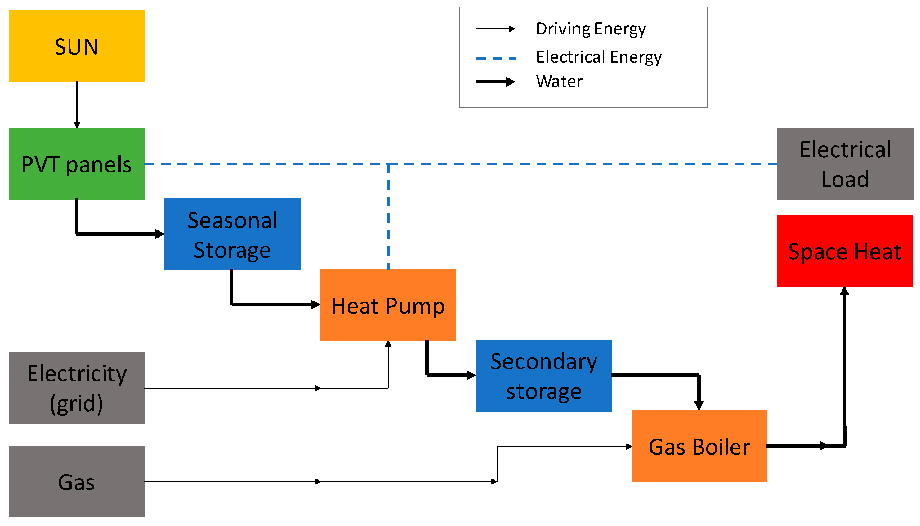
Additionally, since the heat pump is run by electricity, an interesting proposal is substituting the conventional solar thermal panel with hybrid solar PVT panels. Photovoltaic-thermal (PVT) collectors integrate both electricity and hot water production, improving the overall efficiency. In the frame of Task 60 of the IEA [
12], applications of PVT panels are being studied to improve their competitivity over installations that include solar thermal collectors and PV panels. The conceptual scheme is shown in
Figure 1 and has already been implemented in residential and service sectors [
10,
13]. Along with this paper, the hybrid solar system is understood as being a solar energy system based on hybrid photovoltaic-thermal (PVT) collectors. It is understood as a hybrid because it is a solar cogeneration with two independent systems: thermal and electrical, with their corresponding auxiliary devices.
The adequacy of the solar-assisted heat pump (SAHP) for the residential sector and the alignment of these schemes with Task 44 of the Solar Heating and Cooling (SHC) program of the International Energy Agency (IEA) is clear. Different studies face the energy analysis of these systems and indicate positive results both from technical and economic perspectives [
15]. During the last years, numerous studies have been developed in the field of applications of SAHP. Bukert [
16] carried out a full review of SAHP for low temperatures applications. Huan et al. [
17] studied the coupling possibilities of both systems, solar and heat pumps, to optimize energy production. Yang et al. [
18] showed the viability of providing space heating for a residential building by implementing the SAHP system. The difference between community-scale and building-scale when considering long-term storage is pointed out by [
19]. The losses are reduced due to the proximity between solar generation and seasonal storage. Most papers refer to conventional solar collectors [
20,
21], and PVT panels have also been considered in the most recent literature [
22,
23,
24].
However, there exists a gap in the literature when exergy analysis is considered. Different authors have gone through the exergy analysis of PVT panels. Still, there is not much research about the coupling of solar plus heat pumps and seasonal storage. Exergy analysis allows detecting, identifying, and quantifying where and when irreversibility happens [
25]. Therefore, it is useful for improving the design and operation of energy systems. A key point within the exergy analysis is its capacity to measure different nature streams in the same units. In this sense, it is highly recommended to assess the solar cogeneration system studied here.
On the one hand, some works can be found in the literature with the exergy simulation of PVT systems. They usually conduct studies of the performance of the systemd under different climate conditions, and the comparison between single PV and PVT operations is commonly presented as well. In particular, exergy analysis of PV and PVT was developed by Saloux et al. [
26]. Kallio and Siroux [
27] conducted an energy and exergy analysis of the PVT performance in different European weather conditions. The dynamic model of the water-cooled PVT collector was implemented in Matlab/Simulink.
On the other hand, the exergy analysis of solar energy storage (SES) has been analyzed as well. Rezaie et al. [
28] designed an SES to complement and to increase the effectiveness of the solar panels included in a district energy system. Shabgard et al. [
29] considered a residential building in a hot zone and presented an in-depth analysis of a heating, cooling, and hot water system with evacuated tube collectors, a latent heat thermal energy storage unit, and related heat exchangers, and an absorption chiller/heat pump. The inclusion of a phase change material (PCM) layer of a solar heating system has been introduced to analyze the viability analysis of the solar systems with seasonal storage [
30].
Energy and exergy analyses have also been widely applied to deeply analyze energy systems based on other renewable sources and the combination of conventional and renewable technologies [
31,
32]. Different works evaluating the biomass gasification-based multigeneration system’s performance can be found in the literature [
33,
34]. Furthermore, Wu J. et al. [
35] studied the viability of a combined cooling, heating, and power system based on solar thermal biomass gasification throw exergy and exergoeconomic analysis. Beretta presented a detailed allocation of resources and products in a hybrid system [
36]. The thermoeconomic cost of renewable-based hybrid trigeneration (heat, electricity, and desalinated water) has been studied by Calisse et al. [
37]. Some other polygeneration configurations are found in [
38,
39,
40,
41], with the application of exergy cost theory. Different water technologies and desalination techniques can also be found in literature associated with exergy analysis and renewable sources [
41,
42].
After considering the primary mass and energy balances, exergy and exergy cost analyses are proposed in this paper as methods for the complementary assessment and better understanding of the efficiency of a solar-assisted heat pump (SAHP) system combined with seasonal storage. The solar field is composed of hybrid solar panels, which means a step further in the utility’s conception and engineering. Many authors present solar systems considering either thermal solar or photovoltaics. With the same solar field surface, this proposal allows combining the advantages of both thermal advantage and electricity support to the projected heat pump. Through the exergy-based analysis, the profit obtained by storing thermal energy in summer and consuming it in winter is quantified. The study is performed month by month and for the whole year for a system that supplies heating in a social housing building situated in Zaragoza, Spain. In addition to the presented simulation and second principle-based analysis shown in this work, essential support to the study presented in this paper is the SAHP system with seasonal storage, which is currently under construction at the University’s San Francisco Campus of Zaragoza, Spain. The monitoring of the system will provide valuable information to validate the model and reinforce the results of this paper.
2. Materials and Methods
Although the exergy and exergy cost analysis is the final target of the research work presented in this paper, the previous steps in the global analysis are briefly explained to provide the complete framework. Details can be found in [
43].
The work started with meetings in the city court to get precise information from the original project to simulate the building under consideration. Design Builder [
44] is an integrated set of in-depth, high-productivity tools to assist in the simulation of buildings. It allows getting the yearly demand for construction after introducing all constructive features of the building and its expected use. In this way, the original construction project was used to define the building’s enclosures and differentiate the zones according to their use. The thermal and electricity demands are defined by introducing specific average data records from the consumption habits of the end-users. Thermal demand includes both DHW and heating. Electricity requirements were also obtained. The schedule of heating and the setting temperatures at different periods were also considered in the simulation.
The characterization, study, and dynamic analysis of the building and its demands (electricity, heat, and DHW) were the key starting points for the dynamic simulation of the proposed SAHP plus seasonal storage. The system was modeled and analyzed in TRNSYS [
45], a specific software used to obtain detailed information about the energy system performance along the year. It is a flexible graphically based software widely used to simulate the behavior of transient systems, especially systems run by solar [
46,
47]. The energy system was organized into five parts to get a structure able to reproduce its performance accurately. The main components are the solar field, the seasonal storage water tank, the heat pump, and the water tank of the hot side of the HP that supports the heating demand of the building (secondary tank). Many other auxiliary devices, both mechanic and electrical, are included.
Finally, a socio-economic and environmental global analysis was carried out to provide broad and multi-perspective information to compare the proposed system with other alternatives. Fundamental performance ratios and exergy and exergy cost indicators were calculated every year.
Since the project is located in Spain, legal and technical requirements defined by the Technical Building Code (Código Técnico de la Edificación—CTE) [
48] were observed. Technical specifications of the project relating to heating and cooling installations are reflected in the regulation of thermal installations in buildings (Reglamento de Instalaciones Térmicas en los Edificios—RITE) [
49].
TRNSYS output files were organized to be manageable in the exergy and exergy cost analysis. An independent Excel sheet was used for this purpose.
2.1. Components and Energy Balances
Six specific subsystems were defined to explain in detail the components and the operating mode of the energy system. They are depicted in
Figure 2: (i) Solar field: PVT + solar pump + pipes; (ii) seasonal storage: cold tank; (iii) heat pump + cold loop + pump 1 + hot loop + pump 2; (iv) buffer: hot tank + pump demand; (v) boiler; and (vi) grid (electricity from/to the grid).
The solar loop comprises the solar field, the impulsion and return pipes, the solar pump, and the additional small devices required to operate the system, such as valves and security elements. This subsystem’s primary input is the irradiance of the sun, and the outputs are the heat and the electricity produced by the solar field (QPVT and WPVT, respectively).
The seasonal storage tank stores the heat collected in the solar loop throughout the year and constitutes the cold side of the heat pump (
QCF). The input in the seasonal storages is determined after subtracting the losses of the solar loop (
Qloss_solarloop) from the heat obtained in the solar field (
QPVT):
The block of the heat pump is composed of the cold loop (the circuit that takes heat from the seasonal storage (
QCF) and drives it to the evaporator of the heat pump) the heat pump body, and the hot loop that connects the condenser of the heat pump with the buffer. This buffer is secondary storage that allows for a backup to provide the heat demand properly. The heat from the HP into the buffer is
QHP and constitutes the hot side of the heat pump. The buffer provides heat to the heating circuit (
Q).
QHP is the input to the buffer, and
Qdem_HP is the output from the buffer. The boiler is activated (
Qaux) when the heat provided by the heat pump (
Qdem_HP) is not sufficient to meet the demand (
Qdem). The energy system is, therefore, connected to the gas network.
The interaction of the system with the grid is relevant since the electrical demand of the heat pump (WHP) may not coincide with the electricity production in the solar field (
WPVT). The following balances apply both instantly and for the yearly values. The values with the “grid” subscript mean electricity consumption/demand is different from the heat pump. They are always lower than the total of the building.
The performance of the heat pump is determined by its coefficient of performance (COP), defined as the ratio between the
QHP and the electricity consumed by the compressor (Equation (5)).
2.2. Exergy Analysis
The simulation model described above is based on the first law of thermodynamics. However, several authors already started using the second law approach [
50,
51] to complete their analyses. The second law can be included in the analysis using the concept of exergy, which quantifies the maximum work that a given flow or amount of matter or energy could produce while interacting with the environment. In other words, exergy indicates the quality of energy and matter flows. For instance, electric energy is pure exergy. However, to obtain thermal exergy, the temperature at which it is delivered concerning the environment must be considered.
Accordingly, the output files from TRNSYS were used to determine the exergy flows according to the literature regarding exergy calculation. Exergy of sun radiation is obtained by applying the well-known approach proposed by Petela [
52,
53], as indicated in Equation (6).
where
I is the solar intensity, A is the surface area, and
To and
Ts are temperatures of reference and of surface-emitting radiation (both in K). The author assimilated extra-atmospheric solar radiation with undiluted blackbody radiation. A bunch of studies deeply analyzing the exergy of solar radiation can be found in literature, both from a general perspective [
54,
55] and for the application of specific locations [
56,
57]. The use of Petela’s approach has been discussed by some authors [
58]. It should be noted that the reference temperature for exergy calculations in this energy system has been made equal to the soil temperature, taking in mind that the piping system of the municipal water supply network is buried. The value slightly varies along the year.
The exergy of water flow is defined by its mass flow and six parameter measurements that characterize the physical conditions of water: temperature, pressure, composition, concentration, velocity, and altitude. The exergy method associates each parameter with its exergy components: thermal, mechanical, chemical, kinetic, and potential [
59]. In the studied case, the only relevant component is the physical exergy of water and water-glycol streams, since no chemical reactions and kinetic and potential energies are negligible. Furthermore, the dynamic simulation does not explicitly consider pressure drops. It is possible to assume incompressible flow with constant specific heat. Accordingly, the exergy of water and water-glycol streams can be calculated as (Equation (7)).
where m is the mass flow rate,
c is the specific heat, and
T and
T0 are temperatures of the flows and reference, both in K. Finally, the exergy of natural gas is assumed equal to its lower heating value [
60].
In this paper, exergy analysis (and also thermoeconomic analysis) were applied during given periods (one month or the whole year). For this reason, the exergy mentioned above flows (in kW) must be integrated along these periods:
Besides exergy flows, exergy accumulated in tanks has to be taken into account. This can be done by considering incompressible substance and neglecting variation of pressure as indicated in Equation (9):
In the previous equation, the summation of terms included stratification, leading to temperature variation and the tank.
Mi and
Ti are the mass and temperature of each layer. This is a critical point in the study since, as it is well-known, it improves the performance of stratified sensible thermal energy storage. To obtain precise and useful distinctions between stratified and non-stratified storages and storages at different stratification states, analyses that incorporate second law considerations should be included. A detailed review of studies in which stratification contributes to such storage performance was assessed by [
61] based on energy and exergy analyses. Fertahi [
62] published a review of experimental and numerical studies on stratified storage tanks for individual and collective solar hot water production applications. They face two different approaches: the three-dimensional CFD approach and the two-dimensional formulation based on introducing the vorticity stream function equation. A set of thermal performance indicators commonly used by the scientific community was taken to assess its thermal yield. Haller et al. [
63] presented an exciting review focused on the methods used to determine storage ability to promote and maintain stratification during charging, storing, and discharging. They represented this ability with a single numerical value in terms of a stratification efficiency for a given experiment or under given boundary conditions. They pointed out the difficulty of the existing methods to allocate the entropy production caused by mixing and the entropy changes due to heat losses. Some other authors have devoted their attention to consider specific applications such as the building sector [
64], the relevance of the geometry of the thermal storage, or the search for the best sustainability indicators to make solar heat, including storage, a cost-effective method to meet the increasing energy demand of the industrial sector [
65].
Given a component within a system, flows entering, and leaving the system (and also exergy terms related to accumulation) can be classified into fuel (
F) and product (
P). The product includes the flows associated with the purpose of the system, whereas fuel(s) are the flows consumed to obtain that purpose. It should be highlighted that this classification goes beyond exergy analysis by introducing the idea of the purpose process [
66]. Difference between fuel and product corresponds to irreversibility (
I), or the exergy destroyed;
Besides exergy efficiency, the parameter that computes the effectiveness of a system relative to its performance in reversible conditions is the quotient between product and fuel (Equation (11)):
Due to the second law of thermodynamics, some exergy is destroyed in every real process. Accordingly, irreversibility is positive, and exergy efficiency is lower than 1. The lower the irreversibility and the higher the efficiency, the better the process from a thermodynamic point of view.
Attending to the specific process may occur, where the product sometimes (and, accordingly, the efficiency) is equal to the summation of several terms. This is the case with PVT panels, which coproduce heat and electricity (the increase of the exergy of water-glycol flow and electricity). Additionally, fuel and products of components with accumulation also include terms related to this stored exergy.
2.3. Exergy Cost Analysis
As explained previously, in every process the exergy of the product is lower than the exergy of fuel. In other words, exergy is not conserved. This idea leads to the concept of exergy cost, which is the amount of exergy resources consumed by a system needed for producing a flow of this system. Analyzing the cost formation process along a system can provide valuable information about its efficiency and components.
Symbolic thermoeconomics are applied in this paper to proceed with the exergy cost calculations. It constitutes a methodology for analyzing energy systems based on exergy cost theory and a compact formulation by matrix operators [
66,
67]. It has the advantage of providing the value of exergy cost and analyzing its process formation. In particular, cost formation is analyzed in two complementary ways: (i) according to irreversibility taking place along the productive chain and (ii) according to consumed resources. A short review of the background and main points of the methodology is presented here.
The system under analysis is represented by a productive structure that describes the purpose of the different components. This structure comprises components, and an additional component noted as 0 is included as the environment. Each component consumes resources (fuel, F) from other components or the environment to produce useful effects (product, P). Eij represents a flow that is part of the product of component i and becomes part of the fuel of component j. A table containing elements Eij is the fuel–product table, and its definition is the first step for building a thermoeconomic model.
The amount of exergy resources used to produce this flow is defined as the exergy cost of a flow Eij and is noted as The exergy flow of fuel and product is represented by F* and P*, respectively. The unit exergy cost of a flow is the quotient between its exergy cost and its exergy, and it is represented as k*.
A key point to continue with the methodological framework is the definition of distribution coefficients
yij. They support the thermoeconomic model by quantifying the part of the product of the
jth component that becomes the fuel of the
ith component (Equation (12)). A matrix containing elements
yij is called
.
In [
66], a formulation of cost decomposition of a stream into terms, considering the irreversibility of different components, was developed. It was demonstrated that in a system without wastes, the vector containing exergy cost of the product of all plant components can be calculated as:
where
P* is a vector containing the cost of the product of all components,
P is a vector with the exergy of those products,
UD is the identity matrix,
is the matrix of elements
yij,, and
I is a vector containing the irreversibility of all components. The previous equation indicates that the cost of the products is equal to its exergy plus additional terms due to irreversibility appearing in the different components. In an ideal process without irreversibility, the cost of all products would be equal to their exergy. However, since processes are real, the cost of the product increases. Once exergy cost decomposition is calculated using Equation (13), unit cost decomposition is straightforward by dividing exergy cost into exergy. In this case, unit exergy cost is equal to 1 plus other terms caused by the irreversibility of plant components located upstream in the cost formation process.
In [
68], a different approach to the decomposition of cost is proposed. It is based on the origin of resources consumed by the system. This method is interesting, as in the example analyzed in the paper it includes solar energy, natural gas, and primary energy to generate electricity from the grid.
The first step is to decompose the vector of fuel consumed by the plant (
Fe) into a summation of
nf terms (
kFe), each one corresponding to a different kind of energy (Equation (14)):
With this fuel decomposition, it was shown in [
68] that the cost of the product of all plant components could also be decomposed, as shown in Equations (15) and (16):
where:
where
kP*is the cost of the products due to fuel k,
UD is the identity matrix,
is the matrix of elements
yij, and
kFe is the vector of inputs of a given type of plant fuel. Similar to the decomposition of exergy cost presented in Equation (13), unit exergy cost decomposition can be obtained by dividing exergy cost into exergy.
In the development of this research, the presented equations were introduced in an Excel spreadsheet to go further with the calculation separately. Although exergy calculations could have been introduced in TRNSYS as well, Excel allows for easy implementation of the formulae used for both exergy and exergy cost calculations, as explained next (step by step):
Value of variables needed for exergy calculations (temperatures, flow rates, electricity flows, etc.) provided by TRNSYS for each hour along a year are pasted in an Excel spreadsheet.
The exergy rate of flows (in kW) is calculated in different columns of the same sheet using Equations (6) and (7). Exergy accumulated in tanks (in GJ) is also calculated by applying Equation (9).
The exergy of flows (in GJ) for months and the whole year is calculated by summation, taking into account the time step of 1 h (see Equation (8)).
Fuel and product for each month and the whole year are calculated according to the fuel and product definitions. For the present case study, these definitions appear in
Table 1.
Irreversibility and efficiency are obtained using Equations (10) and (11), respectively.
In order to perform exergy cost calculations, fuel–product tables are required. In the present case, the fuel–product table for the whole year (i.e., without the effect of accumulation) can be seen in
Table 2, whereas the table definition for months (taking into account the effect of accumulation) appears in
Table 3.
matrices are calculated by applying Equation (12).
Product exergy cost formation according to irreversibility is obtained by using Equation (13) and matrix operators of Excel.
Product exergy cost formation according to resources is calculated by Equation (16) and matrix operators of Excel.
Unit exergy cost of products is calculated by dividing the exergy cost of products into their exergy.
Finally, it should be noted that the presented methodology has been developed for the steady-state analysis of systems, that is, without accumulation terms. However, in this paper, the method is being extended to consider the effect of exergy accumulated in tanks. This was done by applying virtual components and an extended fuel–product table, as detailed in
Section 3.3.
3. Case Study
The building considered in this work is a block of social apartments under construction located in Zaragoza, Spain. The council owns it through the municipal institution “Municipal Society Zaragoza Housing” (Sociedad Municipal Zaragoza Vivienda, SMZV), which is devoted to finance and operates the construction within a framework of high efficiency and the Agenda 2030 [
69].
The schema proposed for the energy system (SAHP plus seasonal storage) is especially convenient in this social project because the radiation potential in Spain and Zaragoza is much higher in the summer months than in winter. Obviously, the thermal demand is lower. Therefore, it is necessary to consider taking advantage of that available energy during the summer months by proposing a larger solar installation that stores the energy captured in a large hot water tank (seasonal storage). This stored energy will then be used in winter as the cold source of a heat pump that will provide heating to the building.
This alternative may involve a higher initial cost in the construction of the home than conventional heating alternatives. Still, it means a very significant saving in the home heating system’s operation throughout its useful life. Thus, that solution is an exciting option for social housing in Zaragoza since it is a sector affected by energy poverty. It is fundamental to propose efficient and cheap heating solutions for users.
The building has five floors, and the total constructed surface area is about 7317 m2. The project states that the ground floor houses the common areas (catering, entertainment, offices, etc.), while 80 apartments are planned on the upper floors. There are three different kinds of apartments, depending on the size. Some standard services are also available on each floor (laundry and storage rooms). Each floor will have common areas, a cleaning room, storage, and corridors in addition to the social flats. The roof is the place for the HVAC installation and other equipment.
The dynamic simulation in TRNSYS can be seen in
Figure 3, where demand profiles and specific tap water data were implemented [
70,
71]. The six previously described subsystems were carefully designed and implemented in the software to account for any of the energy facility’s specificities. Special attention was devoted to regulating the heat pump. The operation ranges in both cold and hot sides and is critical to obtaining accurate results. As indicated, the demand profiles obtained from the software Design Builder and tested with previous calculations were introduced in the dynamic simulation as well.
3.1. Energy Analysis
The energy balances explained in
Section 2.1 lead to determining the main energy ratios of the case study. They are developed, presented, and analyzed in [
43]. For the sake of completeness, a short summary of the main outputs is shown here. These figures constitute the exergy analysis background and, consequently, the exergy cost analysis presented in this paper.
The solar potential in Zaragoza on the 90 PVT panels is about 1800 kWh/m
2/yr (south faced and with a slope of 37°). The hybrid solar system takes advantage of its free resource with a thermal utilization ratio of about 25% and an electrical utilization ratio of 18% (raw production). The storage tank volume is 100 m
3, and the heating power of the heat pump is 50 kW. After including the system’s losses and performance, a complete set of energy, economic, and environmental KPI were calculated [
43]. The space heating coverage is 26.7%, and the payback period is about eight years.
3.2. Exergy Analysis
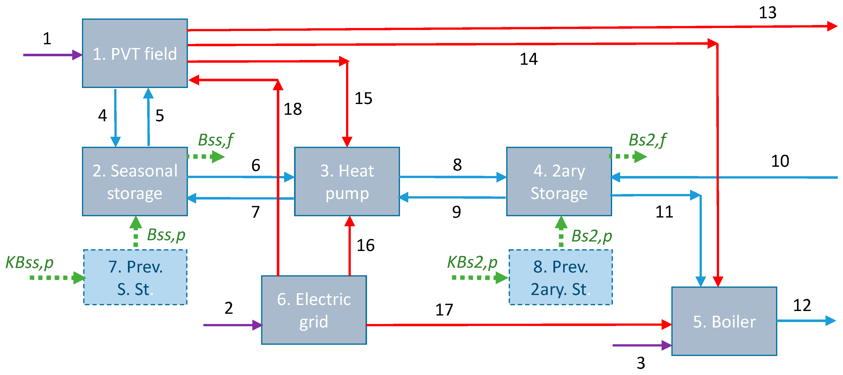
Figure 4 represents a simplified scheme of the system where the components and flows are numbered to enable the application of exergy and exergy cost analyses. Components 1 to 5 represent actual devices or groups present in the plant: PVT field, heat pump, ancillaries (e.g., pumps), storage (seasonal and secondary), and gas boiler. Component 6 is devoted to the electric grid. Finally, 7 and 8 are virtual blocks used in exergy cost analysis to consider the cost of exergy stored at the beginning of each analysis period; their role will be explained later. Flow 1 corresponds to solar radiation; flow 2 is the primary energy needed for producing electricity imported from the grid, and flow 3 is natural gas consumed by the boiler. Flows 4 to 12 are water or water-glycol streams used to transport thermal energy from one component to another. Electric flows are numbered from 13 to 18 and connect electricity sources with demands. In the current configuration, a standard electric node provides electricity for all demands from PVT panels and, when the previous source is not available, from the electric grid. However, for simplifying exergy cost analysis, this common point has been avoided and replaced by direct links between sources and demands. In this situation, electricity produced by PVT panels not consumed within the plant is exported to the building (flow 13). Dotted arrows are related to storage in components 2 and 4: Bss,p and Bs2,p refer to the exergy stored at the beginning of the period (previous situation), whereas Bss,f and Bs2,f are related to the final situation.
The fuel and product of each of the fundamental components presented in
Figure 4 (1 to 6) and the whole plant are defined in
Table 1 using the same nomenclature for the flows. In the table, both fuel and products are classified into four types: heat, electricity, other, and storage. It should be noted that “heat” is actually pairs of flows that allow transferring thermal energy from one component to another. “Storage” flows refer to exergy stored in the seasonal and secondary storage (components 2 and 4). Finally, “others” include solar radiation, primary energy consumed by the electric grid, and natural gas. For instance, PVT consumes solar radiation (B
1) and electricity from the grid (B
18, only in some periods when pumps are in operation, and no solar radiation is present) and produces heat (B
4 − B
5) and electricity (B
13, B
14,, and B
15). The fuel of the seasonal storage includes heat from PVT (B
4 − B
5) and exergy stored at the beginning of the period (B
ss,p).
In contrast, its product is the heat delivered to the heat pump (B6 − B7) and exergy stored at the beginning of the period (Bss,f). Fuel and secondary storage products also include heat (from the heat pump and boiler) and stored exergy (at the beginning and end). The heat pump consumes heat and electricity (from either PVT or grid) and produces heat for secondary storage. The boiler consumes heat from secondary storage, electricity, and natural gas and produces heat, which is a plant product. The electric grid consumes primary energy to produce electricity to be used when PVT generation is not enough. When the whole system is considered, fuel includes sun radiation (B1), primary energy (B2), natural gas (B3), and the initial situation of storage (both seasonal and secondary). The complete system produces electricity (B13), heat (B12 − B10), and exergy stored at the end of the analyzed period.
3.3. Exergy Cost Analysis
The starting point for performing exergy cost analysis is the fuel–product Table, which contains elements E
ij. The methodology is developed for analyzing steady-state systems (in other words, processes without accumulation). The system of this example can be considered as without accumulation if an entire year is analyzed: in this situation, exergy stored at the end of the period would be equal to that of the beginning and, thus, accumulation exergy can be neglected. This can be done by using the fuel–product table defined in
Table 2, where the 6 fundamental components appearing in
Figure 4 are included as well as the environment (component 0). Each row of the table shows how the product of each component becomes part of the fuel of other devices. For instance, PVT (component 1) provides heat for seasonal storage (component 2) and electricity for heat pump (component 3), boiler (component 5), and final plant product.
On the other hand, each column explains how the fuel of each component is made from flows coming from other components or the environment. For example, the heat pump (component 3), consumes heat from seasonal storage (component 2) and electricity from PVT (component 1) and from the electric grid (component 6). It can be seen how total fuel and the product of the different components agree with the definition of fuel and product made in
Table 1, except for terms related to storage, which were removed as explained above.
Due to the transient nature of the analyzed system, it is interesting to also include storage terms in the analysis. The approach is also applied to computable periods where a stationary state is assumed. This can be done by applying a new procedure that is explained below. It is based on the use of an extended fuel–product table (
Table 3), which is based on the previous table (
Table 2) but includes two additional components (7 and 8), which are related to the situation of storage devices in the stage previous to the one being analyzed. Furthermore, additional flows are needed (those represented by dotted arrows in
Figure 4); it can be seen how the table corresponds precisely to the diagram presented in
Figure 4.
The approach can be explained by considering seasonal storage (component 2). When the cost balance of this component is made, exergy stored in the component at the end of the period must have the same unit exergy cost as the other products. This can be done by adding a term to the products of the component, which is flow Bss,f leaving the plant. Besides, the exergy cost balance has to consider that the exergy stored in the seasonal storage at the beginning of the analyzed period is Bss,p. It has the unit exergy cost corresponding to the previous period analyzed (k*ss,p): this can be done by adding component 7, which produces Bss,p and consumes an exergy flow equal to k*ss,p Bss,p. A similar approach is made for secondary storage (component 4) where the additional component 8 has been added.
The methodology consists of applying conventional analysis but using the extended fuel–product table sequentially, starting from the first period (e.g., January), followed by the second, etc. In each period, the value of k*ss,p, and k*s2,p is known from the results of the previous period. The problem appears when the periods are repeated cyclically, such as the 12 months repeated year after year. This can be solved by applying an iterative procedure, considering the initial values for January equal to 1, calculating the whole year and, then repeating the calculation considering the previous values for January equal to those obtained for December. After two or three iterations, values obtained at the end of December are almost equal to those estimated.
4. Results and Discussion
In this section, applying the presented exergy-based analyses to the system under study is presented. First, exergy analysis is tackled. Afterward, exergy cost and its formation are discussed—first for the whole year and, later, monthly.
4.1. Exergy Analysis
This analysis incorporates fuel, product, and irreversibility every month for the whole plant and each component. For the whole plant, fuel, product, and irreversibility are represented in different graphs. When components are analyzed independently, two graphs are usually depicted for each one of them: one including the fuel and the other comprising irreversibility and product. Since fuel is equal to irreversibility plus product, the length of the bars appearing in each pair of graphs would be the same.
Figure 5 shows the fuel of the complete system during the year. It can be seen how, as expected, input due to solar radiation higher increases till July and then decreases. Contributions of natural gas and primary energy for electricity are also very relevant during the cold months. The storage role is smaller because it has low exergy despite its relatively high energy content; it can be seen how exergy is stored in seasonal storage from June to November.
The product of the plant is depicted in
Figure 6. It can be seen how heat for covering the demand is produced during the heating season. During hot months, electricity produced by PVT is high. Its demand is low; accordingly, the plant produces an appropriate amount of electricity. Besides, exergy stored in the seasonal storage appears from April to October. In contrast, the exergy contribution in the secondary storage is much smaller.
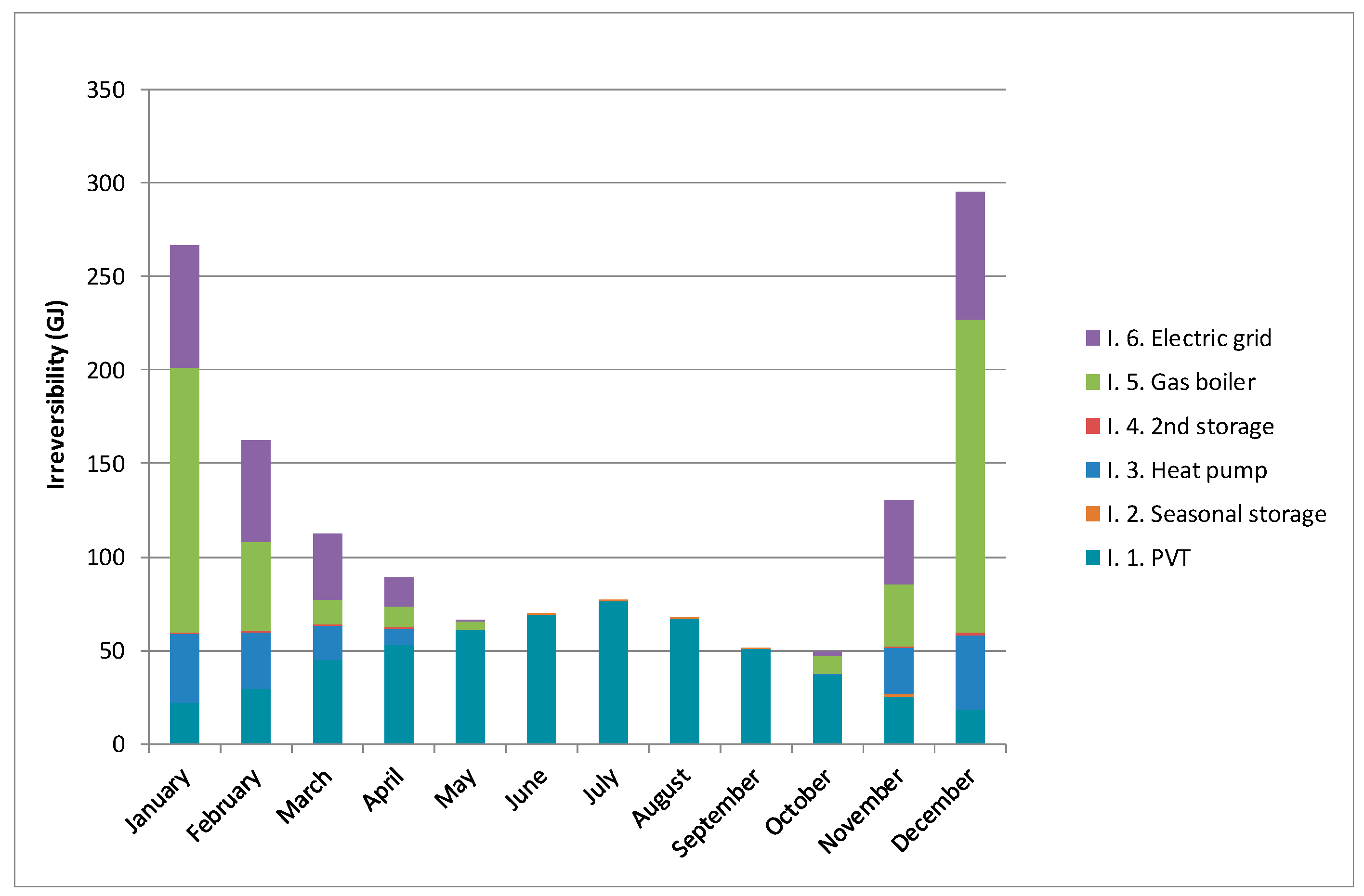
Irreversibility of the complete system appears in
Figure 7. Irreversibility in PVT is higher in sunny months where radiation is also elevated, and this component produces more. Besides, during the heating season, irreversibility appears in components aimed at covering heat demand, such as heat pump and boiler and electric grid, to provide electricity when PVT production is not enough. The contribution of both storage devices is much smaller.
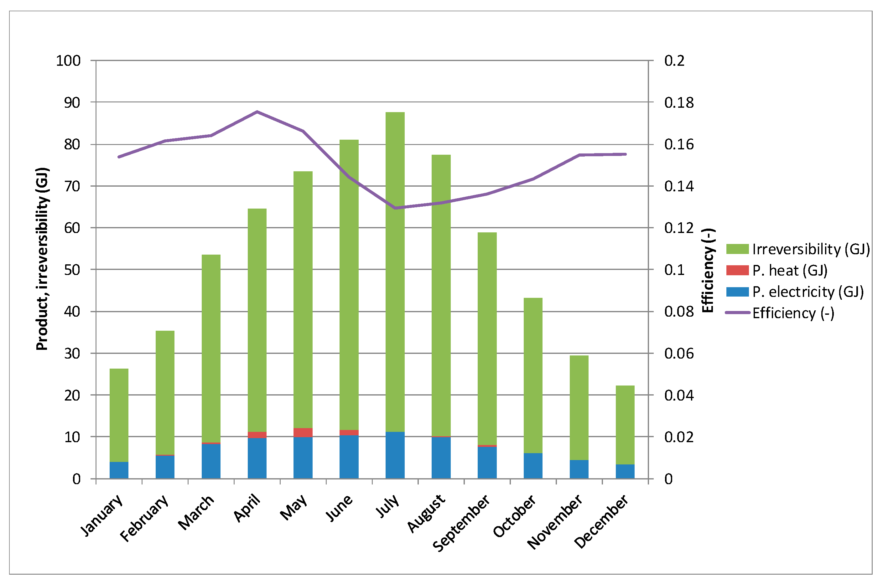
The product and irreversibility of PVT appear in
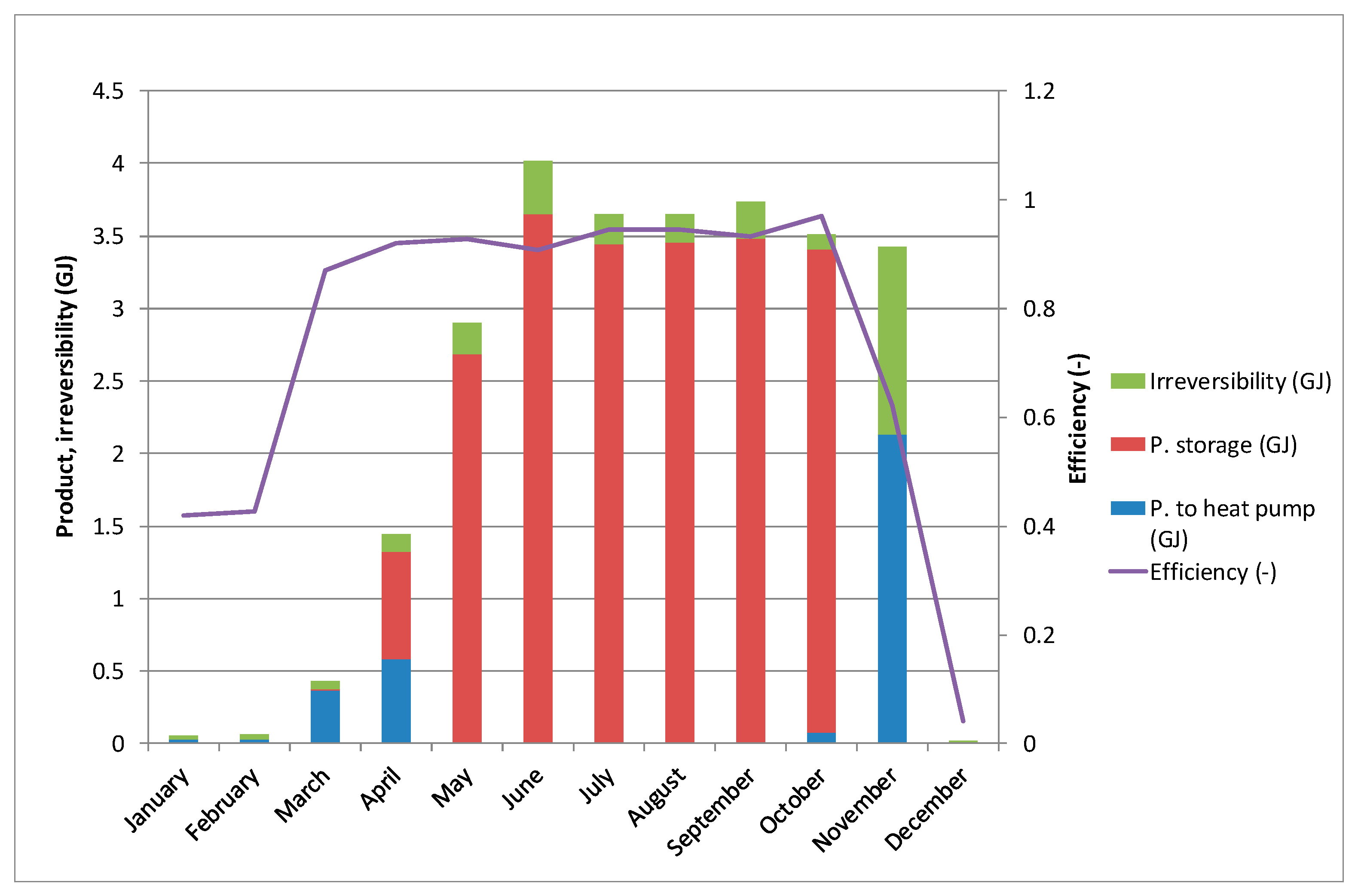
Figure 8. It can be seen that both are higher in sunny months, with higher radiation. Focusing on product, the contribution of electricity is higher than the contribution of heat due to the low temperature of heat, which leads to a low exergy/energy ratio. It may be surprising that the exergy of heat is much lower in July and August than in June, whereas both radiation and electricity produced are similar. This effect appears because once storage has reached a given temperature, the control system acts, and heat produced by PVT is not stored but rejected to the environment. This suggests that it would be interesting to increase the size of that storage in order to be able to accumulate some heat, which with the current design is lost. Besides, the efficiency of PVT is plotted on the same graph. Finally, since in this component almost all fuel corresponds to solar radiation (contribution of electricity from the grid is negligible), it is not needed to plot the bar chart of fuel.
The fuel of seasonal storage is plotted in
Figure 9. In
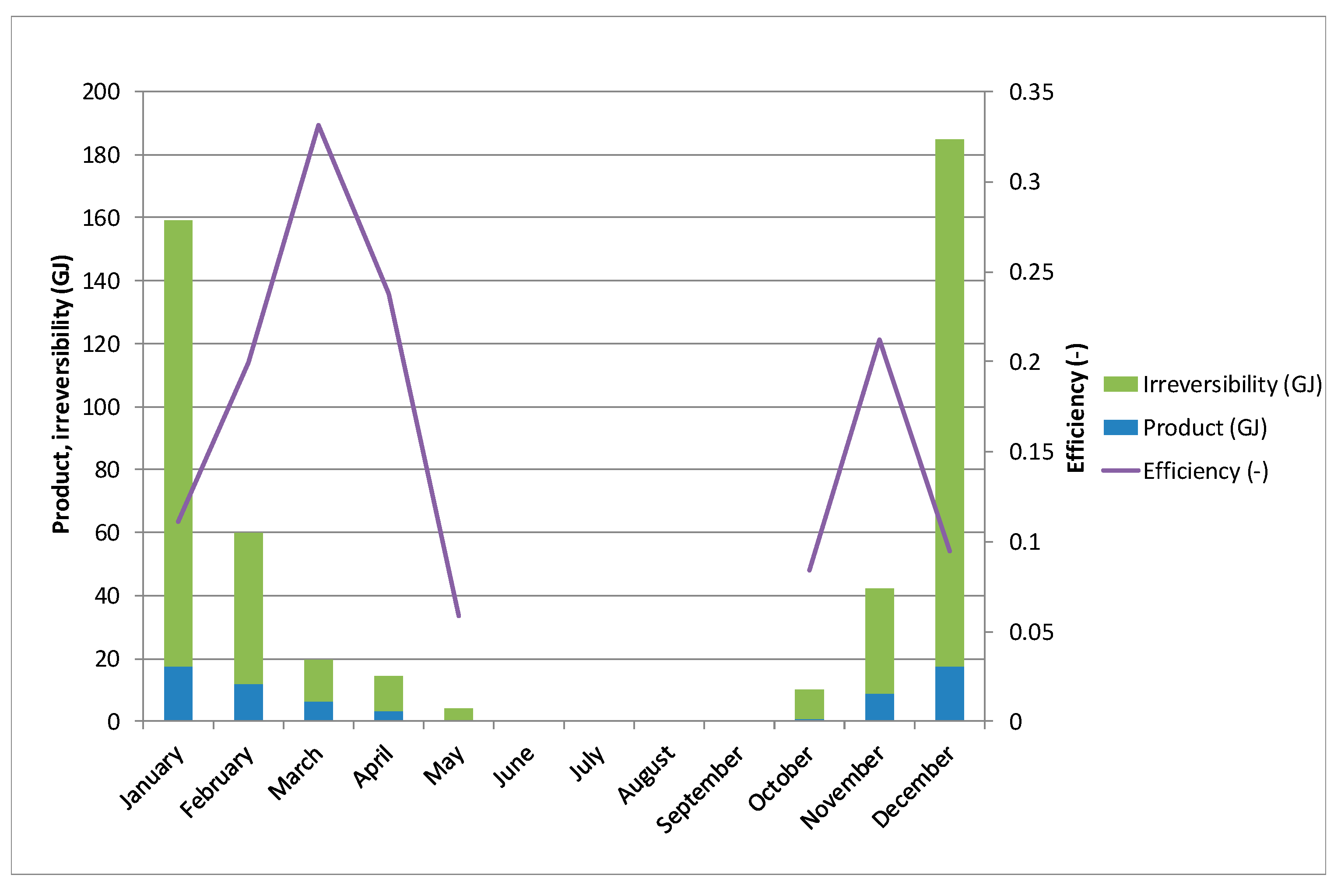
Figure 10, it can be seen when heat is received from PVT (mainly in spring and summer), how the main input is the exergy already stored from previous months, and how this fuel is used as a product or destroyed as irreversibility. When the heat pump is in operation, it consumes resources from the seasonal storage, whereas in summer, the only product is energy stored for later use. The efficiency of this storage is high, except for when the energy stored tends to zero, which means that the temperature in the tank is close to the reference temperature and, thus, exergy is very low.
Figure 11 shows the fuel of the heat pump. It can be seen how the main contribution of this fuel is electricity, because heat from seasonal storage is relevant from an energy point of view but has a low exergy content. The main contribution of heat appears in March and April and, above all, in November. The only product, which is heat to secondary storage and irreversibility and efficiency, is represented in
Figure 12. It can be seen how efficiency is higher in those months when the fuel contribution to heat is more relevant.
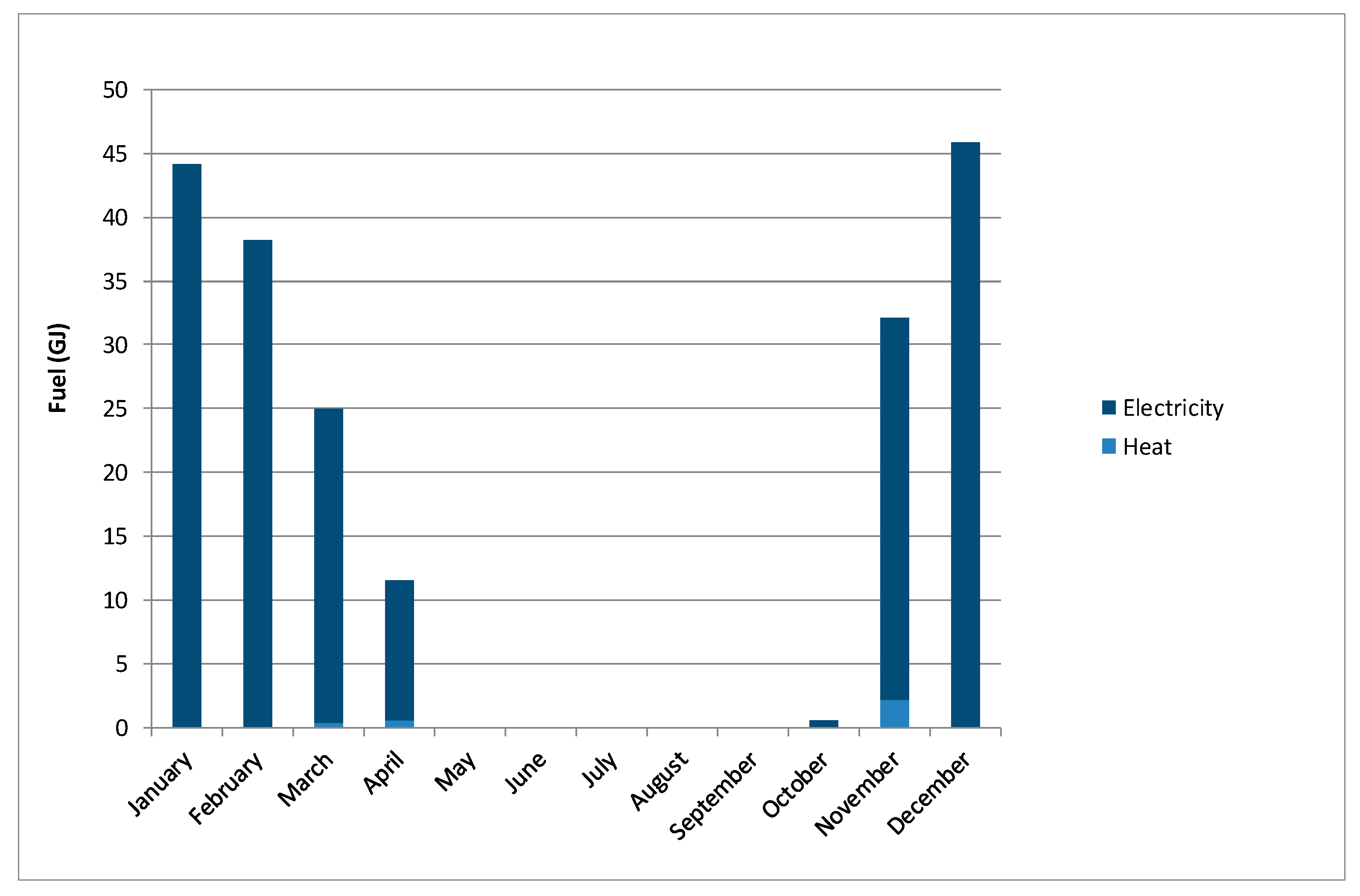
Figure 13 shows the fuel of the gas boiler. It can be seen that the main source is natural gas consumed. This appears because exergy due to the flow heating in the secondary storage is very low compared to its energy. After all, the temperature is low. Besides, some fuel is related to the electricity needed for driving the pumps (it should be noted that this input is included in the boiler, although it also affects secondary storage).
Figure 14 shows how the efficiency of the component increases when the contribution of heat from secondary storage is higher (which reduces the use of natural gas for heating at low temperatures, which is inefficient).
Results of secondary storage and electric grid can be seen in Annex A. In secondary storage, the accumulation contribution is smaller than that of seasonal storage because of its smaller size. The electric grid has a constant efficiency of 0.4.
4.2. Cost Analysis on a Yearly Basis
Unit exergy cost of the products of all components has been first calculated by considering a whole year, which has made it possible to avoid terms related to storage. As presented in the methodology, it is possible to estimate cost decomposition by using two criteria: by cost formation, according to irreversibility taking place along its formation path, and by the origin of resources.
Figure 15 shows the unit exergy cost formation, according to irreversibility for all plant components. It should be noted that these costs would be equal to 1 if only ideal devices (with no irreversibility) were used; this is represented by the label ‘ideal’. The cost of PVT is slightly higher than 6. Its formation is affected only by its own irreversibility because it is located at the beginning of the production chain. The cost of the product of seasonal storage is high, and its formation is affected not only by its own irreversibility but also by the irreversibility of PVT, which is located upstream. The cost of the heat pump product is even higher. It is affected not only by PVT, seasonal storage (slightly), and itself, but also by electricity generation (because sometimes it consumes electricity from the grid). The secondary storage product has a distribution similar to that of the heat pump but a higher value due to irreversibility taking place in the own secondary storage. The boiler product includes heat produced by gas burning and heat produced in the heat pump (this heat was considered fuel for the boiler); accordingly, all plant components present contribution. Finally, the cost of the product of the electric grid is only affected by its own irreversibility.
Since the plant consumes several resources, it is also interesting to see how the components’ cost is formed by the contributions of these components, which can be seen in
Figure 16. Of course, the value of the cost is the same as that presented in the previous figure. The product of PVT and seasonal storage is formed almost solely by solar radiation. In the heat pump and secondary storage, primary energy for electricity also plays a key role. The product of the gas boiler includes the three sources. Finally, the product of the electric grid only is made from primary energy used for producing electricity.
4.3. Cost Analysis on a Monthly Basis
After the cost calculation of the operation of the system during a whole year, this section aims to present unit exergy cost for each month of the year. To achieve this goal, the methodology developed in this paper dealing with storage requires using the extended fuel–product table.
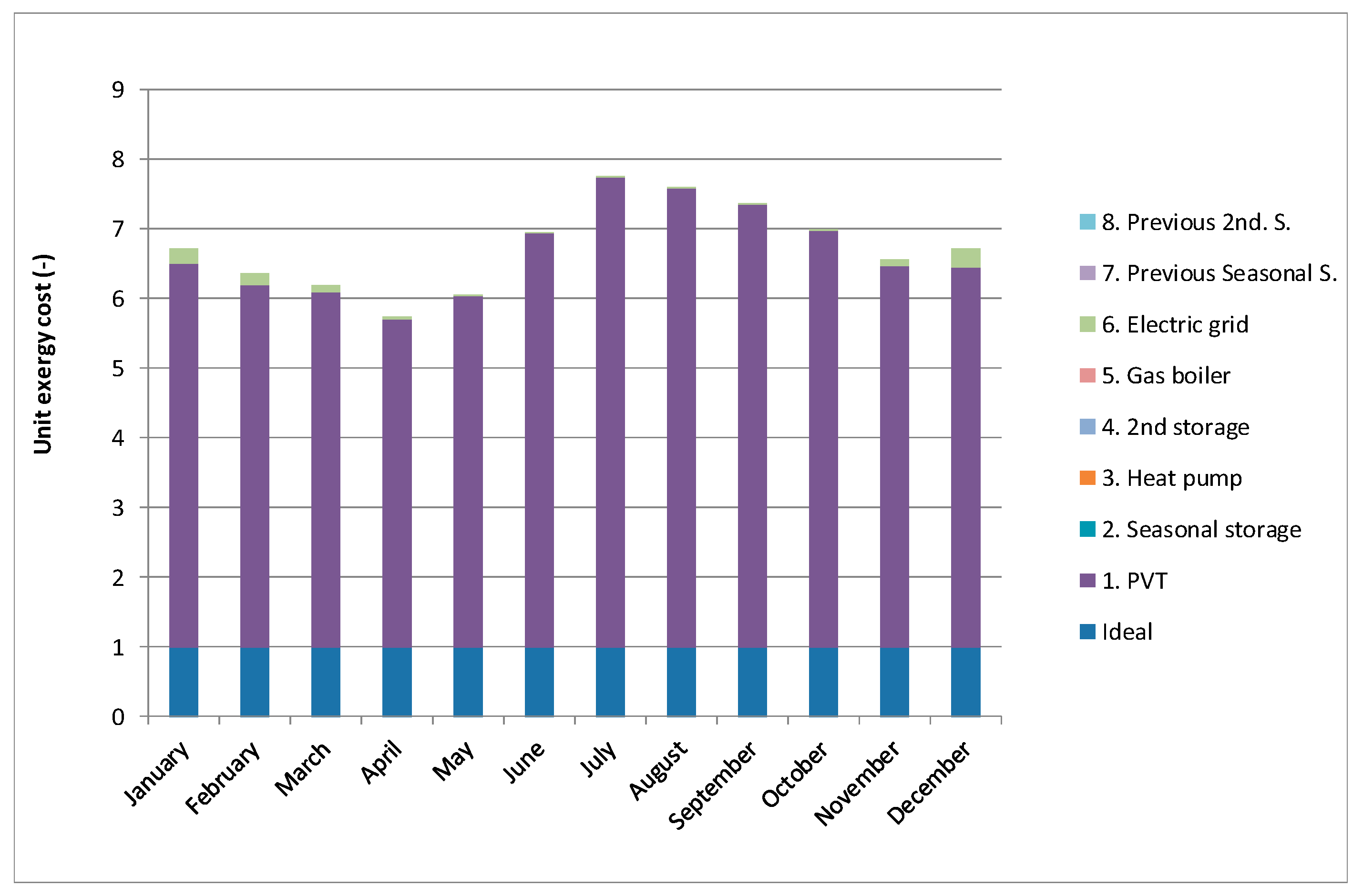
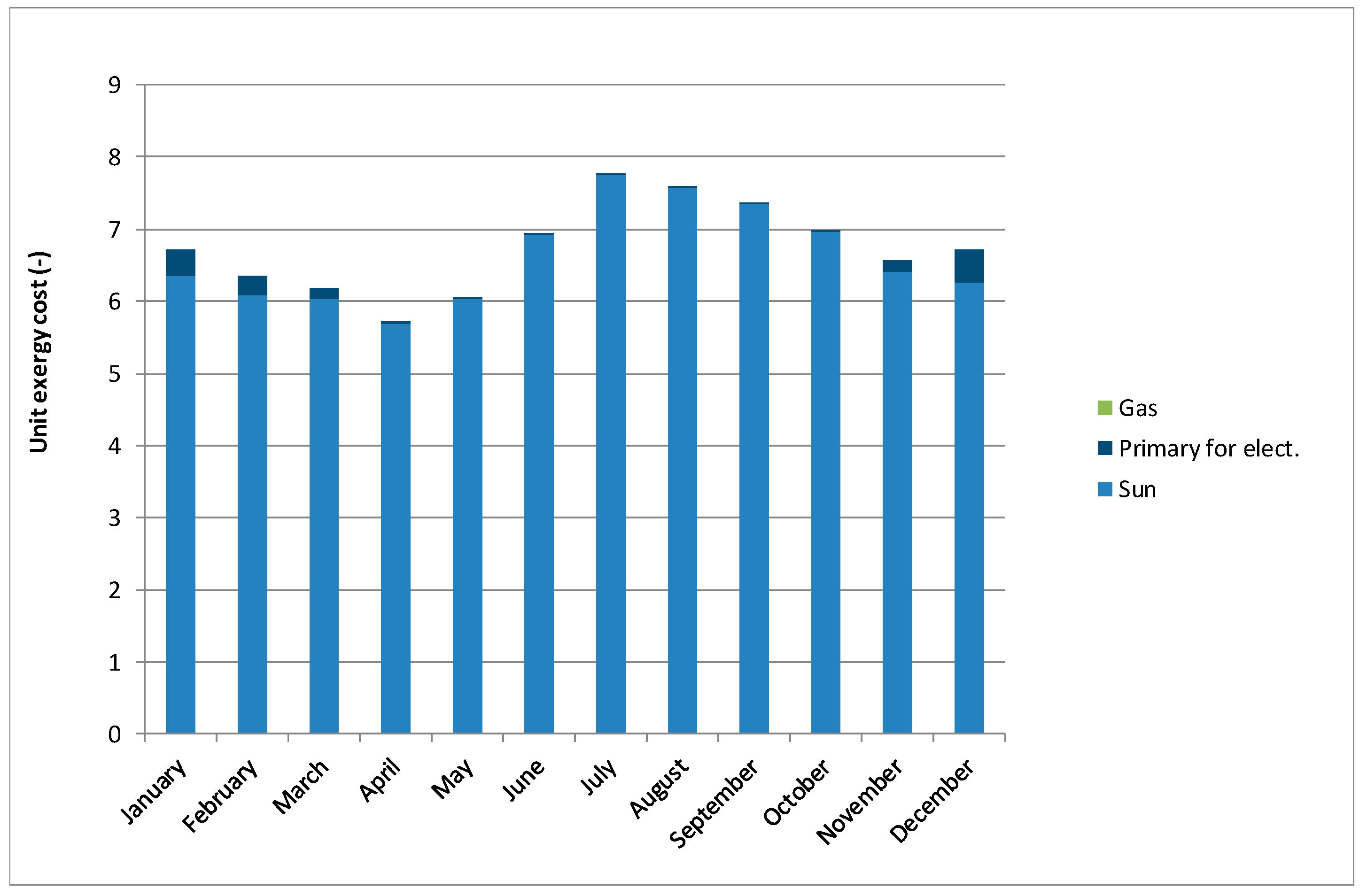
Figure 17 shows the evolution during the 12 months of the unit exergy cost of PVT product according to irreversibility. It can be seen how this cost varies along the year and how it is affected by the irreversibility of the PVT itself and the irreversibility of the electric grid during the months with lower solar irradiation. In those months, sometimes PVT requires electricity from the grid for driving electric pumps. The evolution of the same cost but taking into account the origin of resources is plotted in
Figure 18. The contribution is only solar in all months except for in the colder ones where some electricity from the grid is consumed, as previously mentioned, which is what causes the consumption of primary resources needed for producing this electricity.
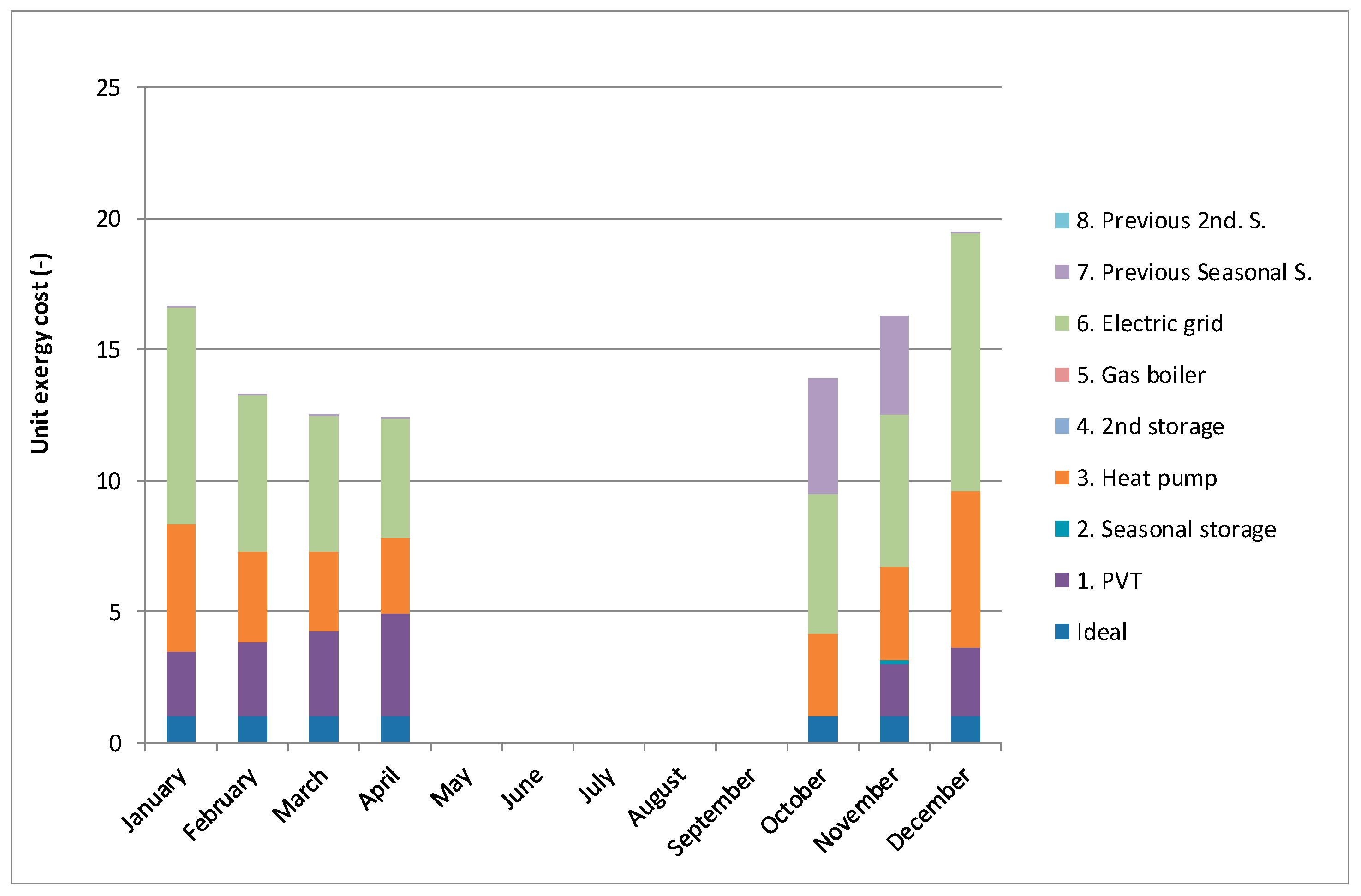
Unit exergy cost of the product of seasonal storage, according to irreversibility, can be seen in
Figure 19. During the first months, the product comes mainly directly from PVT (without relevant storage). Thus, the irreversibility of PVT is the leading cause of cost. However, in summer and autumn, most exergy comes from exergy previously stored (which is represented by component 7, previous seasonal storage). The high value of December’s cost may be surprising; this fact appears because both exergies in the seasonal storage and exergy delivered to heat pump are very low (and, thus, the product is low). Therefore, it makes the cost increase sharply (remember that cost is the amount of resources consumed divided into the exergy of the product).
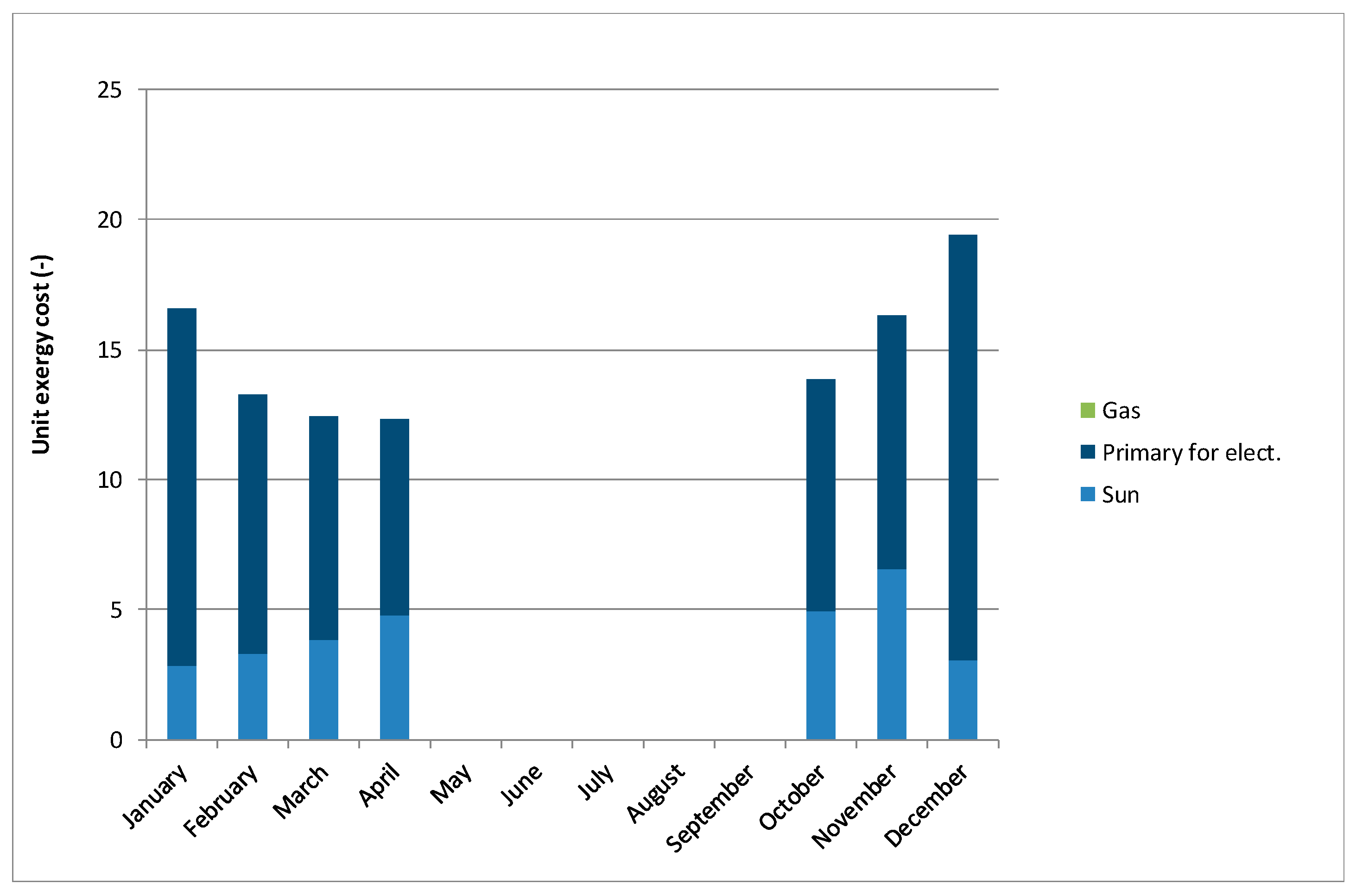
Figure 20 shows how the origin of this cost is almost wholly sun, except for some small contributions of primary energy that appear in cold months (for the same reason explained in the case of PVT). It should be noted that in
Figure 19 and
Figure 20, unit exergy cost for December is represented by using a secondary axis (right side) whereas the main axis (left side) is used for the months from January to November.
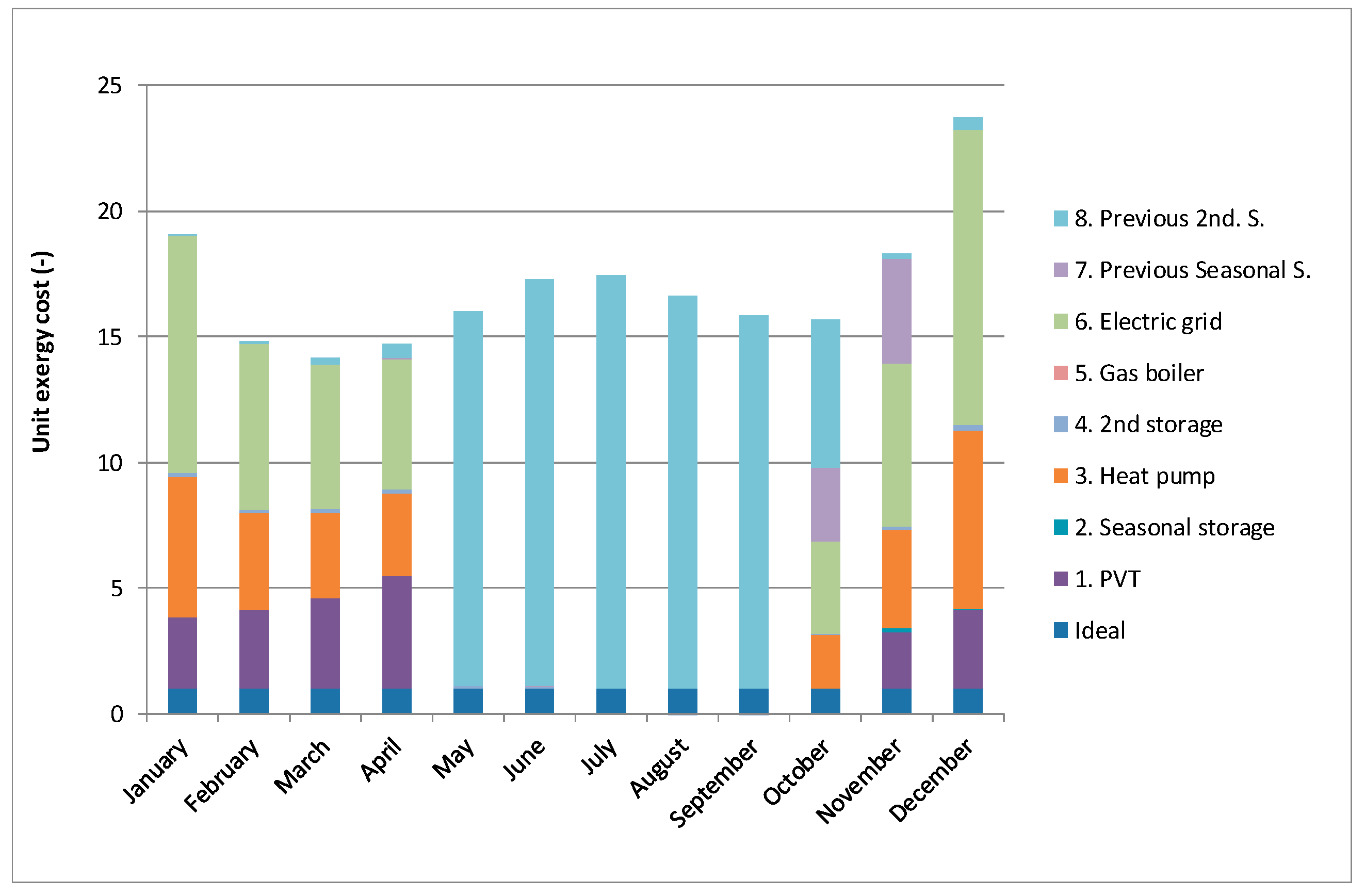
Cost formation of the heat pump, according to irreversibility, is depicted in
Figure 21. First of all, it can be seen that there are no bars during the months in which the heat pump is not in operation. The cost is affected by its own irreversibility, by the irreversibility of the electric grid where part of electricity that consumes is produced and the irreversibility of PVT provides both electricity and heat. In October and November, most heat is consumed from the seasonal storage tank. Thus, the effect of this storage process’s irreversibility also appears.
Figure 22 shows how the cost source is shared between the sun and primary energy for producing electricity; it can be seen how during October and November, the fraction of solar contribution is higher because of the use of thermal energy from the seasonal storage.
The gas boiler is located at the end of the productive process; for this reason, the cost of this product includes the irreversibility of all devices (as can be seen in
Figure 23). This cost is formed from the three resources consumed by the plant (
Figure 24). When the fraction of energy provided by natural gas increases, the relative weight of irreversibility of the boiler also does, and, thus, the contribution of the other components decreases. In November, the previous months’ seasonal storage contribution appears because heat is provided from this storage through the heat pump. The high value of May’s cost may be surprising; this effect occurs because the heating system only works for a few hours and has low efficiency.
The electric grid has a constant efficiency of 40%, and thus, the cost of its product is equal to 2.5. Besides, this cost is only formed by primary resources, which is the only fuel consumed by the component. Finally, cost analysis of the secondary storage can be seen in detail in
Appendix A.
4.4. Main Outcomes
A method for the detailed analysis of exergy cost formation according to resources and irreversibilities for integrated systems with storage has been presented in the present paper. The method is based on the extension of the productive structure by using ‘virtual components’, which represent the situation of devices with storage in the previous step of the analysis. This methodology for including storage is a crucial contribution from both the methodological and application points of view. This method can be easily linked to conventional economic analysis. Thus, it can improve the design of systems that combine different sources of energy and storage to provide heat and electricity for housing. The application of the method has provided detailed information about exergy, exergy cost, and its formation, as has been shown in this section.
It is also interesting to point out some practical results that can be concluded from the study:
It has been seen that in July and August, exergy provided by PVT to seasonal storage is very low. This is because the temperature of the storage tank is high. Thus, the control system releases heat to the atmosphere instead of storing it. This result advises increasing the size of the storage tank to improve efficiency. It should be noted that this modification can also be limited by economic reasons or due to the room available in the building.
The analysis of the cost formation by the source of the product of the boiler (
Figure 24) shows that the contribution of natural gas in May and October is relatively high. In these months, heating demand is low, but the control system switches on the gas boiler quite often. For this reason, it would be interesting to analyze in detail how this control works to increase the contribution of the heat pump, which is more efficient.
Cost formation by the source on a year basis shows that the primary energy for electricity has a relevant contribution to the gas boiler product (which is one of the products of the plant). This contribution depends on the efficiency assumed for the electric grid.
Despite the issues above that need to be improved, results show how the proposed combination of PVT, heat storage, and heat pump allows covering a relevant fraction of the heating demand by using solar energy and, furthermore, during some months, it provides additional electricity for being used in the building.
Finally, it should be noted that results depend not only on the location of the building but also on its characteristics (as well as on the size of the PVT field, heat pump, and storage tank). For this reason, the number of combinations that could potentially be analyzed is very high. Fortunately, the methodology proposed in the paper can easily be translated to any building in any location.
5. Conclusions
The search for the diversification of generation sources and the increase in the percentage of participation of renewable energies in the final energy consumption of homes, together with the saving and rational use of energy, is the energy planning axis for a decarbonized future in cities. This paper presents the exergy and exergy cost analysis of a solar-assisted heat pump with seasonal storage in this research line. The chosen solar technology are hybrid solar photovoltaic-thermal panels, and the building of the case study is currently under construction in Zaragoza, Spain. The analysis carried out in this work means a further step in the comprehensive analysis of the energy system.
From the presented results, it can be concluded that, in exergy terms, the role of the storage is low because of the low storage temperature. Exergy is stored from June to November. Each component of the energy system has detailed the cost formation by source. The higher unit exergy cost is found for the second storage, the gas boiler, the heat pump, and the seasonal storage. The contribution of cost formation of seasonal storage mainly comes from the PVT, as expected, and reaches about 13. Furthermore, the analysis has provided some guidelines for improving the system design, such as using a bigger tank for seasonal storage or an improvement of the control strategy related to the gas boiler.
The nature of the presented system required considers the effect of storage. The methodology has been extended to include this effect through the use of virtual components and an extended fuel–product table. A novel contribution to the cost analysis procedure has been included to account for the transient with coherent results. It has been applied to a real case study of SAHP with seasonal storage and heat pump. The simulation with three integrated software (Desing Builder for energy demands, TRNSYS for dynamic analysis, and Excel for exergy and exergy cost) resulted in monthly and yearly cost figures. In the monthly analysis, terms of accumulation appear. However, on a yearly basis, net accumulation is negligible because the situation at the end of the year is almost the same as that initially. For this reason, no accumulation terms appear when the whole year picture is considered.


