
Improvement of Self-Predictive Incremental Conductance Algorithm with the Ability to Detect Dynamic Conditions


Abstract
1. Introduction
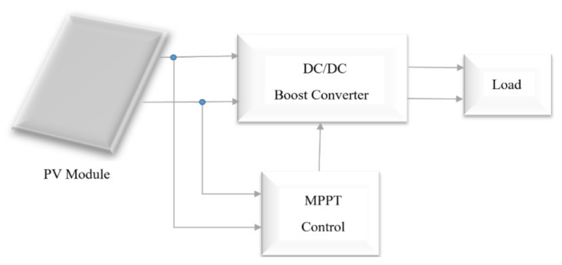
2. PV system Configuration
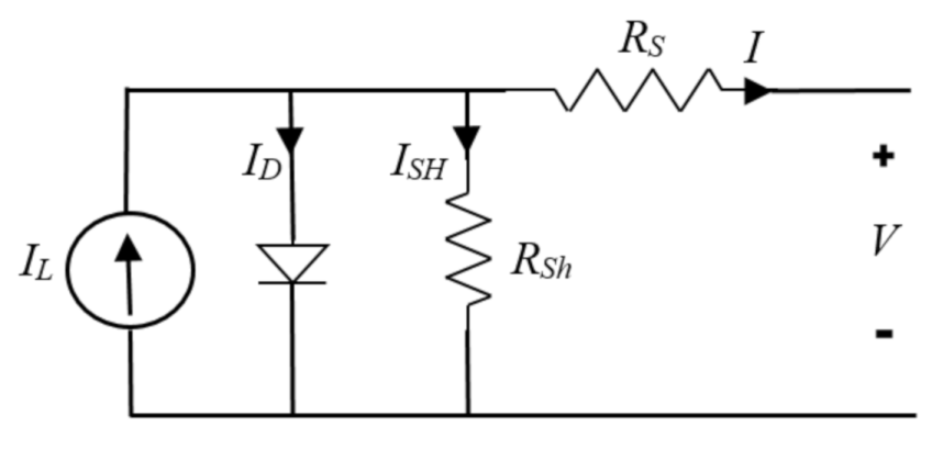
2.1. PV Modeling
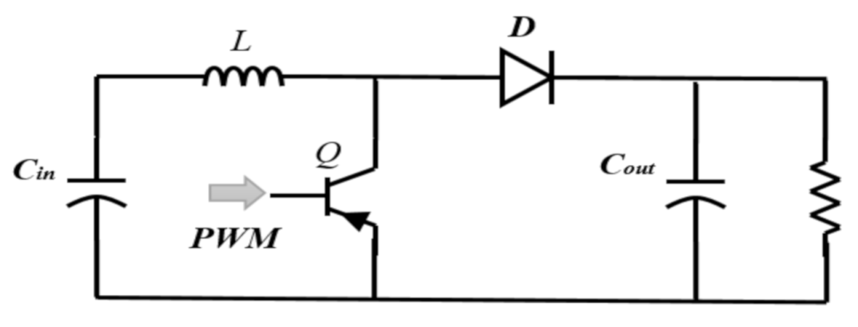
2.2. Boost Converter
3. MPPT
3.1. Conventional InC Algorithm
3.2. Free-Division InC Algorithm
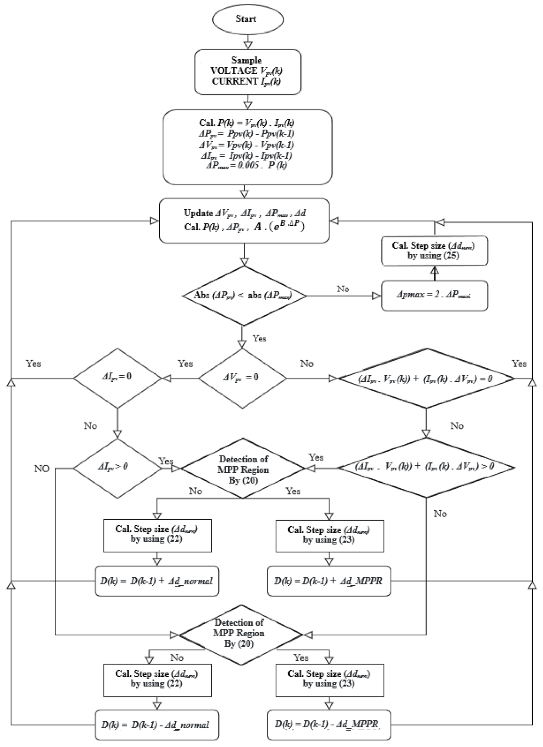
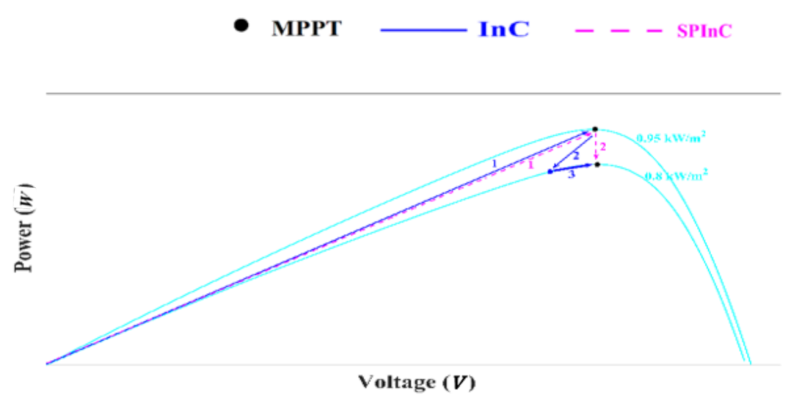
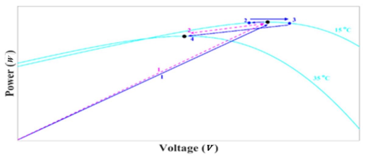
4. Improved Self-Predictive InC
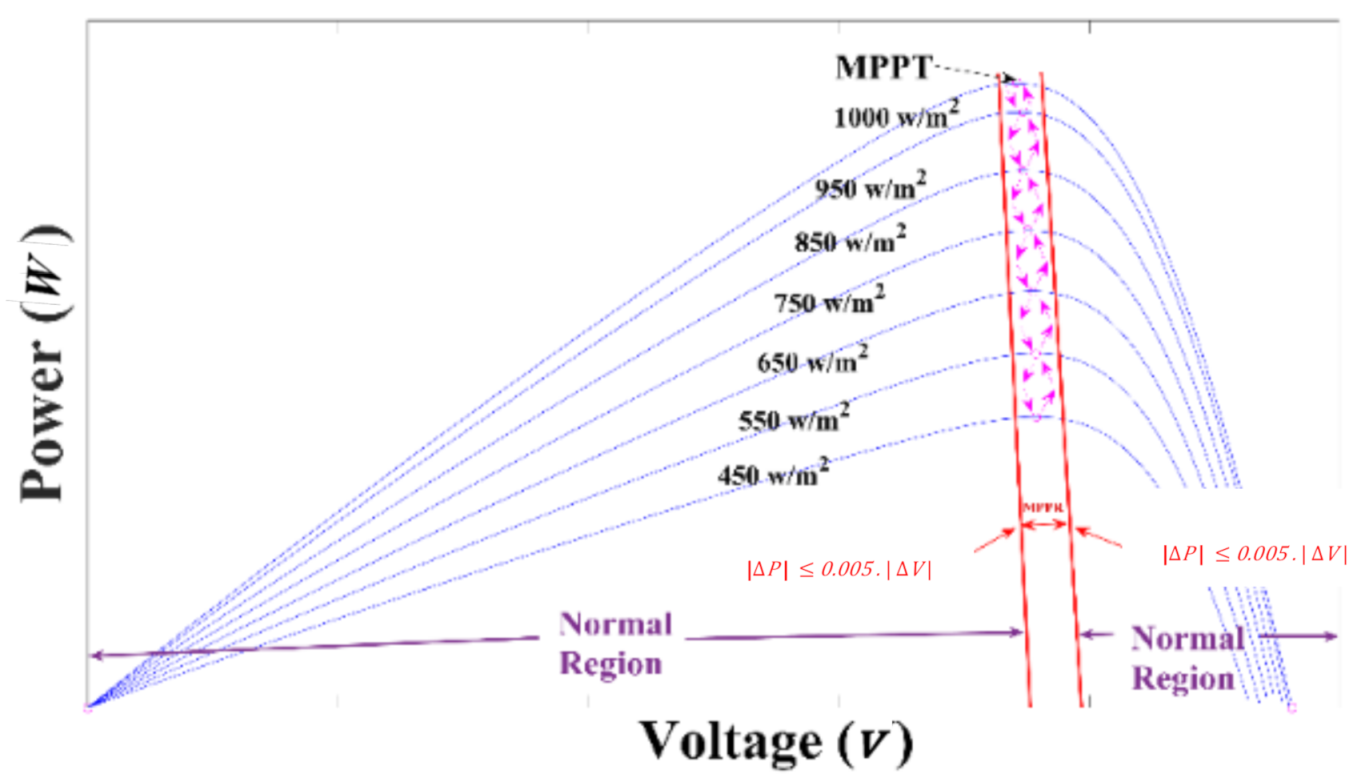
4.1. Detection of MPP Region (MPPR)
4.2. Step Size Determination
4.3. Detection of Dynamic Conditions
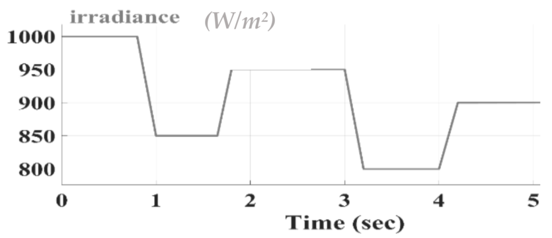
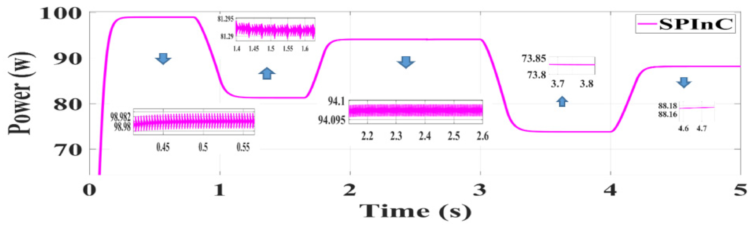
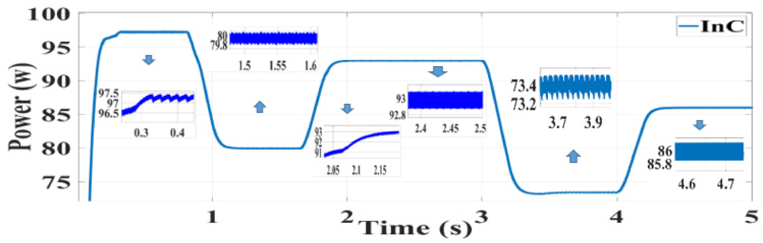
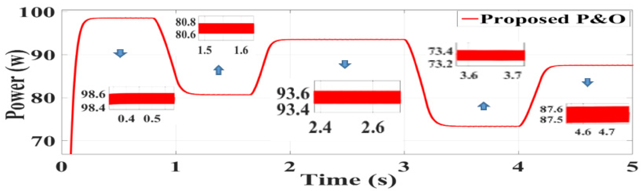
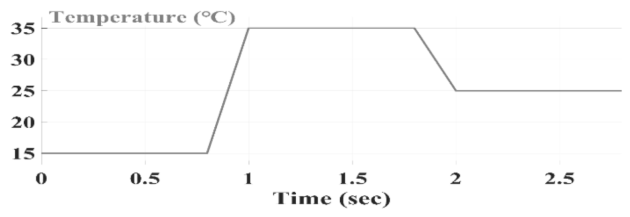
5. Simulation Results
6. Conclusions
Author Contributions
Funding
Institutional Review Board Statement
Informed Consent Statement
Data Availability Statement
Conflicts of Interest
References
- Breeze, P. Power Generation Technologies; Newnes: Oxford, UK, 2019. [Google Scholar]
- Gross, M.; Rüdiger, M. Renewable Energies; Routledge: Abingdon, UK, 2014. [Google Scholar]
- Oncel, S.S. Green energy engineering: Opening a green way for the future. J. Clean. Prod. 2017, 142, 3095–3100. [Google Scholar] [CrossRef]
- Zadeh, M.J.Z.; Fathi, S.H. A new approach for photovoltaic arrays modeling and maximum power point estimation in real operating conditions. IEEE Trans. Ind. Electron. 2017, 64, 9334–9343. [Google Scholar] [CrossRef]
- Kollimalla, S.K.; Mishra, M.K. Variable perturbation size adaptive P&O MPPT algorithm for sudden changes in irradiance. IEEE Trans. Sustain. Energy 2014, 5, 718–728. [Google Scholar]
- Moon, S.; Yoon, S.G.; Park, J.H. A new low-cost centralized MPPT controller system for multiply distributed photovoltaic power conditioning modules. IEEE Trans. Smart Grid 2015, 6, 2649–2658. [Google Scholar] [CrossRef]
- Mohanty, S.; Subudhi, B.; Ray, P.K. A new MPPT design using grey wolf optimization technique for photovoltaic system under partial shading conditions. IEEE Trans. Sustain. Energy 2015, 7, 181–188. [Google Scholar] [CrossRef]
- Liu, C.; Wu, B.; Cheung, R. Advanced algorithm for MPPT control of photovoltaic systems. In Proceedings of the Canadian Solar Buildings Conference, Montreal, QC, Canada, 20–24 August 2004; Volume 8, pp. 20–24. [Google Scholar]
- Faranda, R.; Leva, S. Energy comparison of MPPT techniques for PV Systems. Wseas Trans. Power Syst. 2008, 3, 446–455. [Google Scholar]
- Bahari, M.I.; Tarassodi, P.; Naeini, Y.M.; Khalilabad, A.K.; Shirazi, P. Modeling and simulation of hill climbing MPPT algorithm for photovoltaic application. In Proceedings of the 2016 International Symposium on Power Electronics, Electrical Drives, Automation and Motion, Capri, Italy, 22–24 June 2016; pp. 1041–1044. [Google Scholar]
- Kjær, S.B. Evaluation of the “hill climbing” and the “incremental conductance” maximum power point trackers for photovoltaic power systems. IEEE Trans. Energy Convers. 2012, 27, 922–929. [Google Scholar] [CrossRef]
- Ahmed, J.; Salam, Z. An enhanced adaptive P&O MPPT for fast and efficient tracking under varying environmental conditions. IEEE Trans. Sustain. Energy 2018, 9, 1487–1496. [Google Scholar]
- Ahmed, J.; Salam, Z. A modified P&O maximum power point tracking method with reduced steady-state oscillation and improved tracking efficiency. IEEE Trans. Sustain. Energy 2016, 7, 1506–1515. [Google Scholar]
- Sera, D.; Mathe, L.; Kerekes, T.; Spataru, S.V.; Teodorescu, R. On the perturb-and-observe and incremental conductance MPPT methods for PV systems. IEEE J. Photovolt. 2013, 3, 1070–1078. [Google Scholar] [CrossRef]
- Mei, Q.; Shan, M.; Liu, L.; Guerrero, J.M. A novel improved variable step-size incremental-resistance MPPT method for PV systems. IEEE Trans. Ind. Electron. 2010, 58, 2427–2434. [Google Scholar] [CrossRef]
- Necaibia, S.; Kelaiaia, M.S.; Labar, H.; Necaibia, A.; Castronuovo, E.D. Enhanced auto-scaling incremental conductance MPPT method, implemented on low-cost microcontroller and SEPIC converter. Sol. Energy 2019, 180, 152–168. [Google Scholar] [CrossRef]
- Zakzouk, N.E.; Elsaharty, M.A.; Abdelsalam, A.K.; Helal, A.A.; Williams, B.W. Improved performance low-cost incremental conductance PV MPPT technique. IET Renew. Power Gener. 2016, 10, 561–574. [Google Scholar] [CrossRef]
- Tey, K.S.; Mekhilef, S. Modified incremental conductance algorithm for photovoltaic system under partial shading conditions and load variation. IEEE Trans. Ind. Electron. 2014, 61, 5384–5392. [Google Scholar]
- Guo, Y.; Sun, H.; Zhang, Y.; Liu, Y.; Li, X.; Xue, Y. Duty-Cycle Predictive Control of Quasi-Z-Source Modular Cascaded Converter Based Photovoltaic Power System. IEEE Access 2020, 8, 172734–172746. [Google Scholar] [CrossRef]
- Thangavelu, A.; Vairakannu, S.; Parvathyshankar, D. Linear open circuit voltage-variable step-size-incremental conductance strategy-based hybrid MPPT controller for remote power applications. IET Power Electron. 2017, 10, 1363–1376. [Google Scholar] [CrossRef]
- Elbaset, A.A.; Ali, H.; Abd-El Sattar, M.; Khaled, M. Implementation of a modified perturb and observe maximum power point tracking algorithm for photovoltaic system using an embedded microcontroller. IET Renew. Power Gener. 2016, 10, 551–560. [Google Scholar] [CrossRef]
- Sokolov, M.; Shmilovitz, D. A modified MPPT scheme for accelerated convergence. IEEE Trans. Energy Convers. 2008, 23, 1105–1107. [Google Scholar] [CrossRef]
- Kumar, N.; Hussain, I.; Singh, B.; Panigrahi, B.K. Self-adaptive incremental conductance algorithm for swift and ripple-free maximum power harvesting from PV array. IEEE Trans. Ind. Inform. 2017, 14, 2031–2041. [Google Scholar] [CrossRef]
- Rezk, H.; Aly, M.; Al-Dhaifallah, M.; Shoyama, M. Design and Hardware Implementation of New Adaptive Fuzzy Logic-Based MPPT Control Method for Photovoltaic Applications. IEEE Access 2019, 7, 106427–106438. [Google Scholar] [CrossRef]
- Behera, T.K.; Behera, M.K.; Nayak, N. Spider monkey based improve P&O MPPT controller for photovoltaic generation system. In Proceedings of the 2018 Technologies for Smart-City Energy Security and Power, Bhubaneswar, India, 28–30 March 2018; pp. 1–6. [Google Scholar]
- Hsieh, G.C.; Hsieh, H.I.; Tsai, C.Y.; Wang, C.H. Photovoltaic power-increment-aided incremental-conductance MPPT with two-phased tracking. IEEE Trans. Power Electron. 2012, 28, 2895–2911. [Google Scholar] [CrossRef]
- Belkaid, A.; Colak, I.; Isik, O. Photovoltaic maximum power point tracking under fast varying of solar radiation. Appl. Energy 2016, 179, 523–530. [Google Scholar] [CrossRef]
- De Brito, M.A.G.; Galotto, L.; Sampaio, L.P.; e Melo, G.D.A.; Canesin, C.A. Evaluation of the main MPPT techniques for photovoltaic applications. IEEE Trans. Ind. Electron. 2012, 60, 1156–1167. [Google Scholar] [CrossRef]
- Sekhar, P.C.; Mishra, S. Takagi–Sugeno fuzzy-basedincremental conductance algorithm for maximum powerpoint tracking of a photovoltaic generating system. IET Renew. Power Gener. 2014, 8, 900–914. [Google Scholar] [CrossRef]
- Motahhir, S.; El Ghzizal, A.; Sebti, S.; Derouich, A. Modeling of Photovoltaic System with Modified Incremental Conductance Algorithm for Fast Changes of Irradiance. Int. J. Photoenergy 2018, 2018, 1–13. [Google Scholar] [CrossRef]
- Fesharaki, V.J.; Sheikholeslam, F.; Jahed Motlagh, M.R. Maximum power point tracking with constraint feedback linearization controller and modified incremental conductance algorithm. Trans. Inst. Meas. Control 2018, 40, 2322–2331. [Google Scholar] [CrossRef]
- Jiang, Y.; Qahouq, J.A.A.; Haskew, T.A. Adaptive step size with adaptive-perturbation-frequency digital MPPT controller for a single-sensor photovoltaic solar system. IEEE Trans. Power Electron. 2012, 28, 3195–3205. [Google Scholar] [CrossRef]
- Nasiri, M.; Mobayen, S.; Zhu, Q.M. Super-Twisting Sliding Mode Control for Gearless PMSG-Based Wind Turbine. Complex 2019, 2019, 1–15. [Google Scholar] [CrossRef]
- Bingöl, O.; Burçin, Ö. Analysis and comparison of different PV array configurations under partial shading conditions. Sol. Energy 2018, 160, 336–343. [Google Scholar] [CrossRef]
- Ammar, H.H.; Azar, A.T.; Shalaby, R.; Mahmoud, M.I. Metaheuristic Optimization of Fractional Order Incremental Conductance (FO-INC) Maximum Power Point Tracking (MPPT). Complex 2019, 2019, 1–13. [Google Scholar] [CrossRef]
- Ali, A.I.; Sayed, M.A.; Mohamed, E.E. Modified efficient perturb and observe maximum power point tracking technique for grid-tied PV system. Int. J. Electr. Power Energy Syst. 2018, 99, 192–202. [Google Scholar] [CrossRef]


| Parameters | Label | Value |
|---|---|---|
| Short circuit current | ISC | 1.62 A |
| Open circuit voltage | VOC | 96.2 V |
| Current at Pmax | IMPP | 1.35 A |
| Voltage at Pmax | VMPP | 74.2 V |
| Maximum power | PMPP | 100.17 W |
| VOC coef. of temperature | KV | −0.39 V/°C |
| ISC coef. of temperature | KI | 0.11 A/°C |
| Cells per module | Ncell | 106 |
| Irradiance | 1000 | (W/m2) | 950 | (W/m2) | 850 | (W/m2) | |||
|---|---|---|---|---|---|---|---|---|---|
| Performance Parameters | SPInC | InC | [36] | SPInC | InC | [36] | SPInC | InC | [36] |
| Output power (W) | 98.981 | 97.22 | 98.5 | 94.097 | 93 | 93.5 | 81.292 | 80 | 80.7 |
| Output power ripple (W) | 0.005 | 0.4 | 0.15 | 00.004 | 0.021 | 0.14 | 0.0003 | 0.25 | 0.12 |
| MPPT efficiency % | 98.81 | 97.05 | 98.33 | 98.53 | 97.38 | 97.9 | 94.39 | 92.89 | 93.7 |
| MPPT Technique | Value |
|---|---|
| SPInC | 417.199 J |
| InC | 411.22 J |
| [36] | 415 J |
| Temperature | 15 | °C | 25 | °C | 35 | °C | |||
|---|---|---|---|---|---|---|---|---|---|
| Performance Parameters | SPInC | InC | [36] | SPInC | InC | [36] | SPInC | InC | [36] |
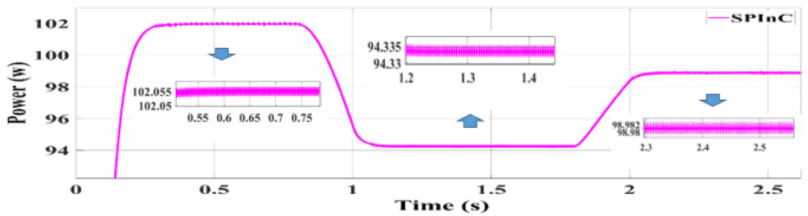
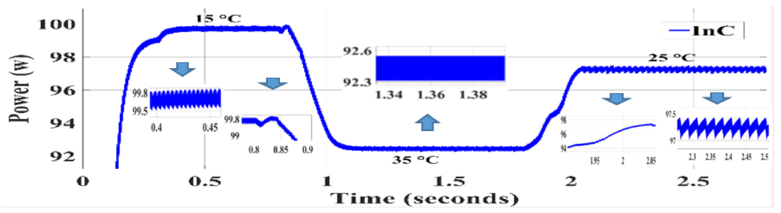
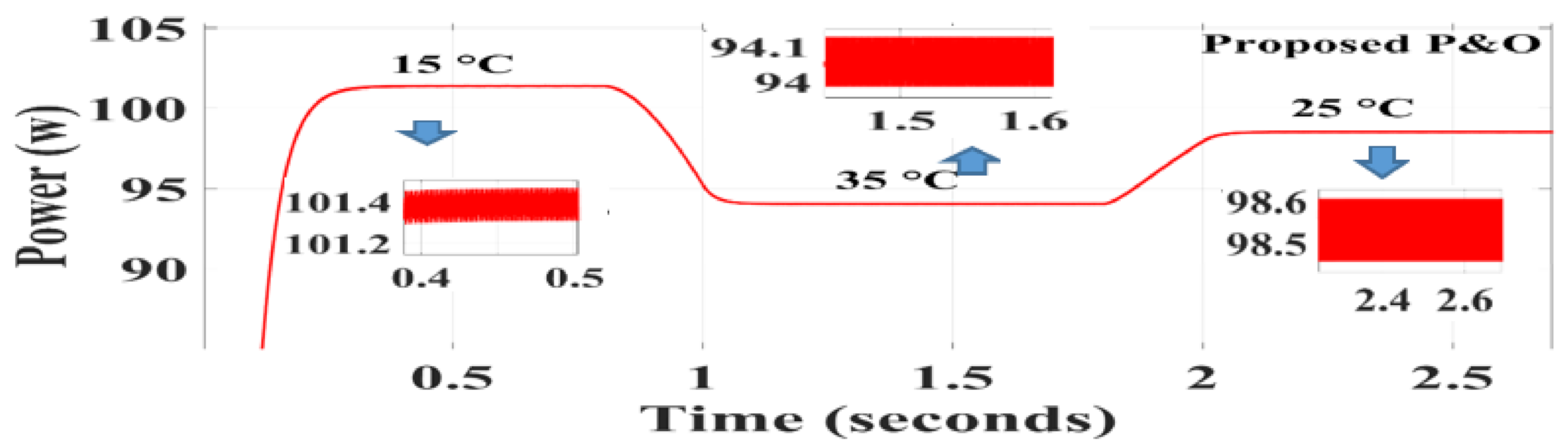
| Output power (W) | 102.05 | 98.7 | 101.4 | 98.981 | 97.22 | 98.55 | 094.33 | 92.43 | 94.05 |
| Output power ripple (W) | 0.005 | 0.35 | 0.16 | 0.005 | 0.4 | 0.15 | 00.003 | 0.25 | 0.14 |
| MPPT efficiency % | 98.3 | 95 | 97.68 | 98.81 | 97 | 98.38 | 98 | 96 | 97.71 |
| MPPT Technique | Value |
|---|---|
| SPInC | 276.503 J |
| InC | 271.38 J |
| [36] | 275.28 J |
| Work | Power Rating | Converter Type | Fsw | MPPT Technique | Power Oscillations | Efficiency |
|---|---|---|---|---|---|---|
| Inc | 100 W | Boost | 5 kHz | Traditional InC | 0.4 W (0.4%) | 97% |
| [27] | 210 W | Boost | ----------- | Adaptive P&O–fuzzy MPPT | 1 W (0.5%) | 95.20% |
| [28] | 250 W | flyback | 40 kHz | PI InC | 14 W (5.6%) | 97.20% |
| [17] | 120 W | Boost | 15 kHz | Modified step-size division-free InC | 4 W (3.33%) | 98.33% |
| [28] | 60 W | Boost | 10 kHz | Modified InC | 1 W (1.67%) | 96.40% |
| [29] | 200 W | Boost | 50 kHz | PI InC | 1.5 W (0.75%) | 98.50% |
| [30] | 30 W | Voltage source converter | 10 kHz | Fuzzy-based InC | 1 W (3.33%) | 97.50% |
| [33] | 10 W | Buck | 100 kHz | Load current based MPPT | 0.04 W (0.4%) | 97% |
| [32] | 5 W | Boost | 20 kHz | Modified InC | … | 98% |
| [31] | 60 W | Boost | 10 kHz | Modified InC | 0.25 W (0.41 %) | 98.80% |
| SPInC | 100 W | Boost | 5 kHz | Self-predictive | 0.005 W (0.005%) | 98.81% |
| division-free InC |
Publisher’s Note: MDPI stays neutral with regard to jurisdictional claims in published maps and institutional affiliations. |
© 2021 by the authors. Licensee MDPI, Basel, Switzerland. This article is an open access article distributed under the terms and conditions of the Creative Commons Attribution (CC BY) license (http://creativecommons.org/licenses/by/4.0/).
Share and Cite
Jalali Zand, S.; Hsia, K.-H.; Eskandarian, N.; Mobayen, S. Improvement of Self-Predictive Incremental Conductance Algorithm with the Ability to Detect Dynamic Conditions. Energies 2021, 14, 1234. https://doi.org/10.3390/en14051234
Jalali Zand S, Hsia K-H, Eskandarian N, Mobayen S. Improvement of Self-Predictive Incremental Conductance Algorithm with the Ability to Detect Dynamic Conditions. Energies. 2021; 14(5):1234. https://doi.org/10.3390/en14051234
Chicago/Turabian StyleJalali Zand, Sanaz, Kuo-Hsien Hsia, Naser Eskandarian, and Saleh Mobayen. 2021. "Improvement of Self-Predictive Incremental Conductance Algorithm with the Ability to Detect Dynamic Conditions" Energies 14, no. 5: 1234. https://doi.org/10.3390/en14051234
APA StyleJalali Zand, S., Hsia, K.-H., Eskandarian, N., & Mobayen, S. (2021). Improvement of Self-Predictive Incremental Conductance Algorithm with the Ability to Detect Dynamic Conditions. Energies, 14(5), 1234. https://doi.org/10.3390/en14051234