Model for Predicting the Operating Temperature of Stratospheric Airship Solar Cells with a Support Vector Machine

Abstract

The stratospheric airship is a kind of aircraft that completely relies on the cycle of photovoltaic energy systems to achieve long duration flight. The accurate estimation of the operating temperature of solar cell modules on stratospheric airship is extremely important for the design of photovoltaics system (PV system), the output power calculation of PV system, and the calculation of energy balance. However, the related study has been rarely reported. A support vector machine prediction method based on particle swarm optimization algorithm (PSO-SVM) was established to predict the operating temperature of solar cell modules on stratospheric airship. The PSO algorithm was used to dynamically optimize the SVM’s parameters between the operating temperature of the solar cell modules and the measured data such as atmospheric pressure, solar radiation intensity, flight speed, and ambient temperature. The operating temperature data of the two sets of solar cell modules measured in the flight test were used to verify the accuracy of the temperature prediction model, and the prediction results were compared with a back propagation neural network (BPNN) method and the simulation results calculated by COMSOL Multiphysics of COMSOL, Inc., Columbus, MA, USA. The results shown that the PSO-SVM model realized the accurate prediction of the operating temperature of solar cell modules on stratospheric airship, which can guide the design of PV system, the output power calculation of PV system, and the calculation of energy balance.

1. Introduction

A stratospheric airship is a flight vehicle that carries a stand-alone photovoltaic power system for long-term steady flight. The energy consumed during a steady flight is harvested using a solar cell array [1,2,3,4]. Therefore, the operating features of the solar cell array directly determine the power that can be harvested with a stratospheric airship. The operating temperature of a solar cell is one of the key factors that affect its power conversion efficiency [5,6]. Predicting the temperature of the solar cell of the stratospheric airship accurately is extremely important for the accurate calculation of the output power of the PV system, and the related energy system design and energy balance calculation. Different types of solar cells have different temperature coefficient that affect their conversion efficiency [7]. The calculation error of the working temperature of solar cell module will lead to the calculation error of its conversion efficiency, and then cause the calculation error of its output power. For example, the flexible thin film solar cell module of copper indium gallium selenium (CIGS) used in stratospheric airship has a temperature coefficient of 0.4%, which means 10 ºC degrees calculation error will cause the calculation error of output power drop 4%. The greater the temperature error, the greater the calculated output power error, which will affect the closed-loop design of the energy system and the energy balance during flight, thereby affecting the flight safety of the airship.

The temperature of a solar cell module will increase during flight due to insolation. Heat tends to be held in the airship as the pressure in the stratosphere is low. The temperature rise in a solar cell module leads to: (1) a reduction in the cell’s voltage and thus its output power, (2) a reduction in solar cell material bandgap and power generation efficiency, and (3) an increase in the capacitive effect of the solar cell, compromising the stability of photovoltaic power generation [6]. A precise model for predicting the temperature of a solar cell is critical in solar cell operating features analysis [5]. Because of the thermodynamic environment with variable factors, the traditional thermodynamic analysis for solar cell modules of airship is complexed. A thermodynamic model of solar cells on a stratospheric airship is shown in Figure 1.

As shown in Figure 1, the temperature of the module increases during operating, which creates a temperature gradient between the solar cell module and the surrounding atmosphere [7,8,9,10]. Heat transfer occurs via the following mechanisms: (1) heat transfer between the solar cell module and the external atmosphere as long-wave radiation; (2) heat transfer between the solar cell module and internal gas in the airship via convection and long-wave radiation; (3) relative motion between the airship hull and the atmosphere, causing convective heat transfer between the solar cell module and its surrounding atmosphere; (4) among the previous three forms of heat transfer, implicit effects have to be considered regarding the convective heat transfer between the airship hull and the atmosphere, atmospheric thermal radiation, and surface long-wave radiation. Due to the complexity of the system and its surroundings, many factors will affect heat transfer. Additionally, because of the effects of low-pressure conditions environment in the stratosphere, the theoretical calculation model of solar cell module thermal properties faces the risk of difficulties in finding solutions and in precisely developing a model.

Many researchers have conducted research about solar cell modules of stratospheric airships. The relationship between solar cell efficiency and temperature of high-altitude long duration airships was studied by Colozza et al. [11]. Furthermore, they designed a cooling system to improve the output performance of the PV system. Garg et al. proposed a method to calculate the solar energy incident on the airship, estimated the area of solar panels that meet the average daily energy demand of the airship, and proposed an optimization method to maximize the output power of solar panels per unit area [12]. Li et al. established a numerical theoretical model to analyze the impact of latitude, date, wind speed and insulation layer on the output power of the solar cell modules, and studied the influence of the PV system on the thermal characteristics of the airship [13,14,15,16]. Wang et al. proposed a method to calculate the solar radiation on the curved solar cell of a stratospheric airship, and studied the influence of the height on the output performance of solar cell modules [17]. Sun et al. proposed a heat transfer model of flexible thin-film solar cells and thermodynamic model of multi-layer insulation material to study the thermal performance of flexible thin-film solar cells on stratospheric airships [18]. Liu et al. proposed an optimization design method for stratospheric airship energy system to conduct the sensitivity analysis of the airship energy system weight and reliability [5]; 1. The operating temperature of a solar cell module on a stratospheric airship needs to be checked against predictions in real flight tests; 2. There are many model parameters required for temperature calculations.

During the actual flight of the airship, the attitude change is non-linear, and the simulation calculation cannot accurately estimate the atmospheric pressure, solar radiation intensity, stratospheric airship flight speed, environmental temperature during the actual flight. Therefore, the operating temperature of solar cell modules and produced energy of PV system calculated by simulation have large errors. A model for predicting the operating temperature of solar cell module that includes measured environmental parameters was developed in this study. Using the same methods applied to ground systems [19,20,21,22,23], the model for predicting the temperature of a solar cell module on an airship is treated as an implicit state estimation problem in a time-varying nonlinear system. The model parameters were obtained using particle swarm optimization algorithm-based support vector machine (PSO-SVM) with a small amount of sample data.

2. Solar Cell Operating Temperature Prediction Model

2.1. Support Vector Machine Principles

Data obtained from actual tests were grouped into training and testing sets. The measured atmospheric pressure (P), solar radiation intensity (G), flight speed (V), and ambient temperature (T_t) were used as the input data x_i = (P, G, V, T_t)_i in this SVM model. The measured solar cell module operating temperature Tc is the output of the model y_i = [T_c]_i, and the training sample set is ${\left\{{\mathit{x}}_{\mathit{i}},{\mathit{y}}_{\mathit{i}}\right\}}_{i=1}^N$. We apply a linear transformation to the nonlinear problem of predicting the temperature of a solar cell. The nonlinear mapping φ(.) is used to map the characteristic vectors from the sample data to a high dimensional characteristic space (Hilbert space). Nonlinear regression is then used on the parameters by using upper bound risk minimization. In the training set, ${\left\{{\mathit{x}}_{\mathit{i}}\right\}}_{i=1}^N$ is an input characteristic vector, ${\left\{{\mathit{y}}_{\mathit{i}}\right\}}_{i=1}^N$ is an output target vector, and we determine a function that describes the relationship between the input characteristic vector and the output target vector in the training sample set as:

$$f\left(x\right)=\omega \cdot \phi \left(x\right)+b,$$

(1)

where ω is the weighting vector, and b is the intercept and b∈R.

The loss function used by the support vector machine is the ε-insensitivity function, where all training data is assumed to follow a linear function under accuracy ε, as defined in the following formula:

$$\left\{\begin{array}{lll}{y}_i-f(x_i)\le \epsilon +{\xi }_i& & \\ f(x_i)-y_i\le \epsilon +{\xi }_i^{\ast }& & i=1,2,\dots ,\mathrm{m}\\ {\xi }_i,{\xi }_i^{\ast }\ge 0& & \hfill ,\end{array}\right.$$

(2)

where ξ_i, ξ_i* are relaxation factors such that both ξ_i and ξ_i* are greater than zero when partition has errors and are zero when the sample partition is error-free.

Corresponding corrections must be applied to the linear regression function under idealized conditions as described above, turning the problem into a minimization problem for optimizing the objective function:

$$\begin{array}{ll}R(\omega ,\xi ,{\xi }^{\ast })=\min \left(\frac{1}{2}{‖\omega ‖}^2+C{\displaystyle \sum _{i=1}^m\left({\xi }_i+{\xi }_i^{\ast }\right)}\right)& \\ s.t.y_i-{\omega }^T\cdot \phi \left(x_i\right)-b\le \epsilon +{\xi }_i& \\ {\omega }^T\cdot \phi \left(x_i\right)+b-y_i\le \epsilon +{\xi }_i& \\ {\xi }_i\ge 0,{\xi }_i^{\ast }\ge 0& \hfill ,\end{array}$$

(3)

the constant C is a penalty factor. Equation (3) can be solved by converting the constraint problem to a Lagrange multiplier problem:

$$\begin{array}{cc}L\hfill & =\frac{1}{2}{‖\mathsf{\omega }‖}^2+C{\displaystyle \sum _{i=1}^m\left({\xi }_i+{\xi }_i^{\ast }\right)}\hfill \\ & -{\displaystyle \sum _{i=1}^m{\mathsf{\alpha }}_i\left(\epsilon +{\xi }_i-y_i+{\mathsf{\omega }}^T\cdot \phi \left(x_i\right)+b\right)}\hfill & \\ & -{\displaystyle \sum _{i=1}^m{\mathsf{\alpha }}_i^{\ast }\left(\epsilon +{\xi }_i+y_i-{\mathsf{\omega }}^T\cdot \phi \left(x_i\right)-b\right)}\hfill & \\ & -{\displaystyle \sum _{i=1}^m\left({\eta }_i\cdot {\xi }_i-{\eta }_i^{\ast }\cdot {\xi }_i^{\ast }\right)}\hfill & \hfill ,\end{array}$$

(4)

where the Lagrange multipliers are α_i and α_i* ≥ 0, and i = 1, 2, m. We then determine the minima of L with respect to ω, b, ξ_i, ξ_i* and the maxima of L with respect to α_i and α_i*. We insert these extrema into L and obtain the maximization function in dual form:

$$\begin{array}{cc}W(\mathsf{\alpha },{\mathsf{\alpha }}^{\ast })& =\frac{1}{2}{\displaystyle \sum _{i=1,j=1}^n({\mathsf{\alpha }}_i-{\mathsf{\alpha }}_i^{\ast })({\mathsf{\alpha }}_j-{\mathsf{\alpha }}_j^{\ast })(x_i\cdot x_j)}\\ & +{\displaystyle \sum _{i=1}^n({\mathsf{\alpha }}_i-{\mathsf{\alpha }}_i^{\ast })y_i}-{\displaystyle \sum _{i=1}^n({\mathsf{\alpha }}_i+{\mathsf{\alpha }}_i^{\ast })\epsilon }\end{array},$$

(5)

subject to the following constraints:

$$\left\{\begin{array}{l}{\displaystyle \sum _{i=1}^n({\mathsf{\alpha }}_i-{\mathsf{\alpha }}_i^{\ast })}=0\\ 0\le {\mathsf{\alpha }}_i,{\mathsf{\alpha }}_i^{\ast }\le C\end{array}\right.,$$

(6)

Equations (5) and (6) are solutions to a quadratic programming problem. Through nonlinear mapping, the input vector is mapped to a high dimensional Hilbert space. Linear regression can be performed in the Hilbert space and transformed back to the original space, giving a nonlinear regression result. Using the Kuhn–Tucker theorem, we have the following at a saddle point:

$$\begin{array}{l}{\mathsf{\alpha }}_i\left[\epsilon +{\xi }_i-y_i+f\left(x_i\right)\right]=0\\ {\xi }_i\cdot {\gamma }_i=0\\ {\mathsf{\alpha }}_{{}_i}^{\ast }\left[\epsilon +{\xi }_{{}_i}^{\ast }-y_i+f\left(x_i\right)\right]=0,\\ {\xi }_{{}_i}^{\ast }\cdot {\gamma }_{{}_i}^{\ast }=0\end{array}$$

(7)

One finds ${\mathsf{\alpha }}_i·{\mathsf{\alpha }}_i^{\ast }=0$, indicating α_i and α_i* cannot both be zero simultaneously. We also find the following:

$$\begin{array}{cc}W(\mathsf{\alpha },{\mathsf{\alpha }}^{\ast })& =\frac{1}{2}{\displaystyle \sum _{i=1,j=1}^n({\mathsf{\alpha }}_i-{\mathsf{\alpha }}_i^{\ast })({\mathsf{\alpha }}_j-{\mathsf{\alpha }}_j^{\ast })(x_i\cdot x_j)}\\ & +{\displaystyle \sum _{i=1}^n({\mathsf{\alpha }}_i-{\mathsf{\alpha }}_i^{\ast })y_i}-{\displaystyle \sum _{i=1}^n({\mathsf{\alpha }}_i+{\mathsf{\alpha }}_i^{\ast })\epsilon }\end{array},$$

(8)

For a standard support vector, provided that ${\mathsf{\alpha }}_i\cdot {\mathsf{\alpha }}_i^{\ast }=0$, then ${\xi }_i=0$ and b can be calculated using (9):

$$\begin{array}{l}(C-{\mathsf{\alpha }}_{\mathbf{i}}){\xi }_i=0,\\ (C-{\mathsf{\alpha }}_{\mathbf{i}}{}^{\ast }){\xi }_i{}^{\ast }=0\end{array}$$

(9)

Similarly, for a standard support vector satisfying $0<{\mathsf{\alpha }}_{\mathbf{i}}{}^{\ast }<C({\mathsf{\alpha }}_{\mathbf{i}}=0)$, we have

$$b=y_i-{\displaystyle \sum _{x_j\in SV}({\mathsf{\alpha }}_j-{\mathsf{\alpha }}_j{}^{\ast })x_j\cdot x_i}-\epsilon ,$$

(10)

Generally, for all standard support vectors, we respectively calculate values of b and take an average:

$$\begin{array}{cc}b=& \frac{1}{N_{NSV}}\left\{{\displaystyle \sum _{0<{\mathsf{\alpha }}_i<C}[y_i-{\displaystyle \sum _{x_j\in SV}({\mathsf{\alpha }}_j-{\mathsf{\alpha }}_j^{\ast })K(x_j,x_i)-\epsilon }]}\right.\\ & \left.+{\displaystyle \sum _{0<{\mathsf{\alpha }}_{\mathbf{i}}^{\ast }<C}[{\mathbf{y}}_{\mathbf{i}}-{\displaystyle \sum _{{\mathbf{x}}_{\mathbf{j}}\in SV}({\mathsf{\alpha }}_{\mathbf{j}}-{\mathsf{\alpha }}_{\mathbf{j}}^{\ast })K({\mathbf{x}}_{\mathbf{j}},{\mathbf{x}}_{\mathbf{i}})-\epsilon }]}\right\}\end{array},$$

(11)

The aforementioned SVM regression method uses an inner product to map to a higher dimensional Hilbert space. To prevent a dimensionality catastrophe caused by relatively large sample size, we use a kernel function instead of an inner product.

We map the input quantity x to a high dimensional Hilbert space H with the mapping relation$\Phi :R^n\to H$, and the data (x_i, y_i) where i = 1, 2, ……, n is fit to the function $f\left(\mathit{x}\right)=\omega \mathsf{\cdot }\Phi \left(\mathit{x}\right)+\mathit{b}$. Thus, Equation (5) becomes:

$$\begin{array}{cc}W\left(\mathsf{\alpha },{\mathsf{\alpha }}^{\ast }\right)& =-\frac{1}{2}{\displaystyle \sum _{i=1,j=1}^n\left({\mathsf{\alpha }}_i-{\mathsf{\alpha }}_i^{{}^{\ast }}\right)\left({\mathsf{\alpha }}_j-{\mathsf{\alpha }}_j^{{}^{\ast }}\right)\left(\Phi \left(x_i\right)\cdot \Phi \left(x_j\right)\right)}\\ & +{\displaystyle \sum _{i=1}^n\left({\mathsf{\alpha }}_i-{\mathsf{\alpha }}_i^{{}^{\ast }}\right)y_i}-{\displaystyle \sum _{i=1}^n\left({\mathsf{\alpha }}_i+{\mathsf{\alpha }}_i^{{}^{\ast }}\right)\epsilon }\end{array},$$

(12)

This equation involves a dot product operation in a high dimensional Hilbert space $\Phi \left({\mathbf{x}}_{\mathbf{i}}\right)\cdot \Phi \left({\mathbf{x}}_{\mathbf{j}}\right)$, where the function Φ is of high dimension and is unknown. Considering a dot product in a high dimensional Hilbert space $K\left({\mathbf{x}}_{\mathbf{i}},{\mathbf{x}}_{\mathbf{j}}\right)=\Phi \left({\mathbf{x}}_{\mathbf{i}}\right)\cdot \Phi \left({\mathbf{x}}_{\mathbf{j}}\right)$, the function Φ is not used directly. We take $K\left({\mathbf{x}}_{\mathbf{i}},{\mathbf{x}}_{\mathbf{j}}\right)$ as a kernel function such that this function represents a dot product in a high dimensional Hilbert space.

$$f\left(x\right)={\displaystyle \sum _{i=1}^m\left({\mathsf{\alpha }}_i-{\mathsf{\alpha }}_i^{\ast }\right)\cdot K\left(x_i,x_j\right)}+b,$$

(13)

In this paper, we selected a Gaussian radial basis function (RBF) as the kernel function:

$$K\left(x_i,x_j\right)=\exp \left(-\frac{{‖x_i-x_j‖}^2}{2{\sigma }^2}\right),$$

(14)

where σ defines the width of the RBF.

The parameters that need to be optimized are the insensitivity loss function ε, penalty factor C, and the RBF width σ. σ reflects the range of training data, which has a greater impact on model prediction accuracy. ε is an important feature of SVM, which determines the number of support vectors and ensures the sparsity of the solution. C is a compromise between model complexity and generalization ability, which determines the level of punishment for samples whose error is greater than ε. When C→∞, the goal of model optimization reduces to experience risk minimization. When C is too small, the proportion of experience risk and the complexity of model structure are declined, But the training error is increased [24].

2.2. Optimizing Parameters in the SVM Model Using Particle Swarm Optimization

The particle swarm optimization algorithm was used to optimize and solve for the model parameters in the SVM model.

The fundamental principle of particle swarm optimization algorithm is to simulate the process by which birds flock while searching for food. Birds are abstracted as small particles (dots) and extend into a q-dimensional space. The definite position of a particle i in this space is represented by a vector ${\mathit{D}}_i={\left[d_{i1}{d}_{i2}\cdots d_{iq}\right]}^T$, and its flight velocity is represented by the vector ${\mathit{V}}_i={\left[v_{i1}{v}_{i2}\cdots v_{iq}\right]}^T$.

The updating method used in particle swarm optimization is described below.

A swarm of random particles are initiated (random solution), and the optimized solution for these particles is found through iteration. In each iteration, particles update their positions by tracking two extrema. These are the historical optimal values pbest_i = (pbest_i1, pbest_i2,..., pbest_iq), where i = 1, 2, 3,..., n, and the optimal values from all particles gbest = (gbest₁, gbest₂,..., gbest_q).

After searching for these two optimal values, a particle updates its own position and flight velocity s as defined below.

$$\begin{array}{l}{v}_{i+1}=\lambda v_i+c_1\times rand\times (pbes{t}_i-x_i)\\ +c_2\times rand\times (gbes{t}_i-x_i)\end{array},$$

(15)

$$x_{i+1}=x_i+v_i,$$

(16)

λ is the coefficient of inertia; c₁ is the weight coefficient of the particle’s correlation with its own historical optimal value, which indicates the degree of the particle’s cognition of itself, and the value is generally 2; c₂ is the particle’s correlation with the group’s optimal values that indicates the degree of awareness a particle has of the group, and its value is generally 2; rand is a random number in the interval (0,1). In Equation (15), the first term is called the “memory item”, which describes the relationship between the particle’s flight speed and the magnitude and direction of the previous speed; the second term is called the “self-cognition item”, which describes the best vector that the particle currently points to, indicating the corresponding action of the particle from its own experience; the third term is called the “group cognition item”, which describes the vector from the current particle pointing to the best of particles, indicating the optimal information sharing between particles. Particles determine their next movement through their own experience and the best experience delivered by their companions. Figure 2 shows the optimization solving scheme.

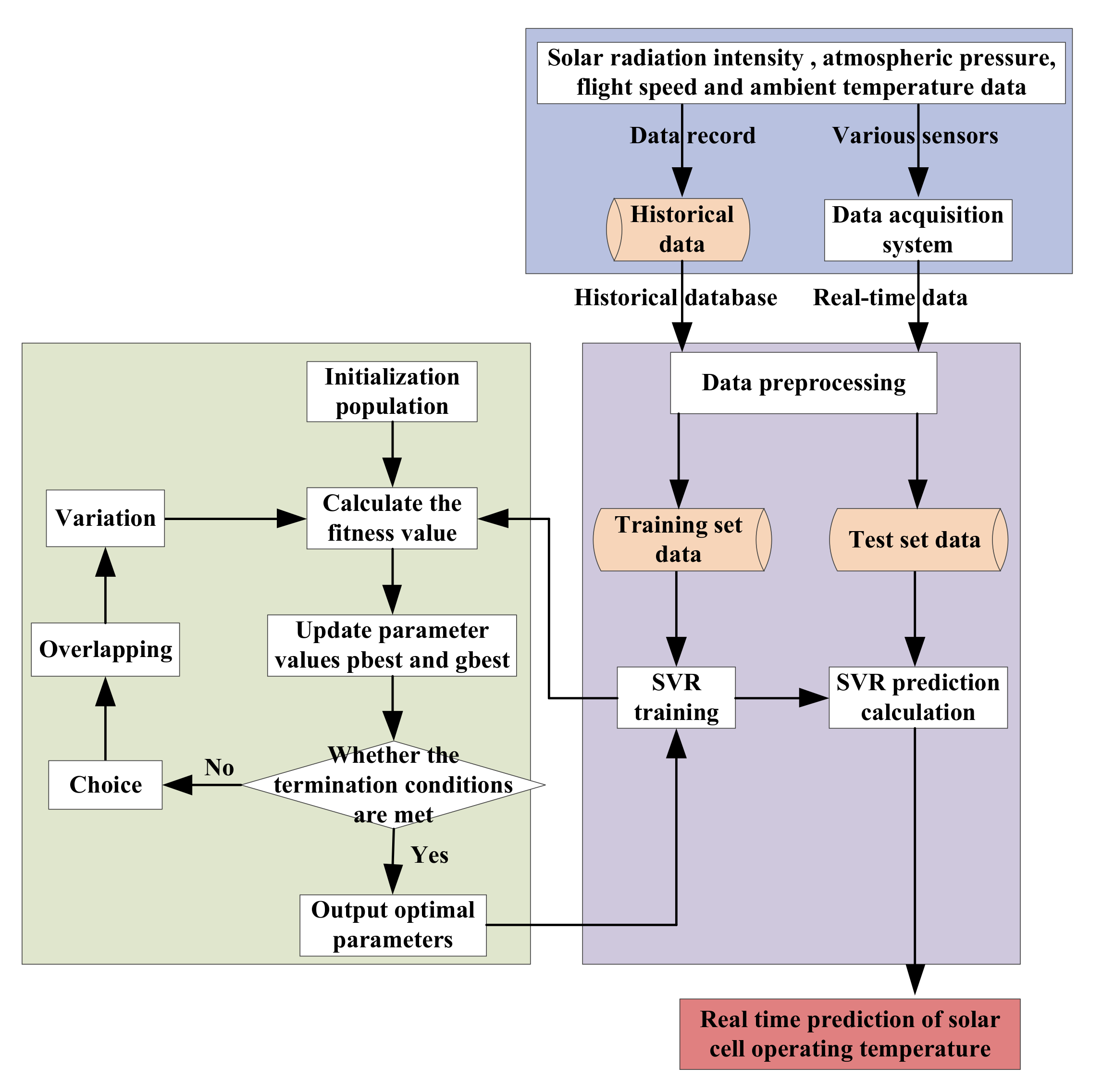
2.3. Solar Cell Temperature Prediction with PSO-SVM

A flowchart showing the use of PSO-SVM for predicting the solar cell temperature during operation is shown in Figure 3. The solar cell operating temperature, solar radiation intensity, atmospheric pressure, flight velocity, and ambient temperature were measured during a flight test were used as sample data and were partitioned into training and testing sets. The training set was used to train the algorithm and determine the optimal model parameters; the testing set was used to assess the accuracy of the established temperature prediction model and determine whether the temperature prediction model should be applied to subsequent calculations depending on assessment results.

We used root-mean-square error (RMSE) between the predicted and measured temperature values to describe the prediction accuracy of the PSO-SVM algorithm.

$$E=\sqrt{\frac{1}{N}{\displaystyle \sum _{j=1}^N{\left(y_{mj}-y_j\right)}^2}},$$

(17)

The process for training the PSO-SVM algorithm can be summarized as follows:

(1)

Sample data is partitioned into training and testing sets, with each set containing solar cell operating temperature as function of solar radiation intensity, atmospheric pressure, flight velocity, and ambient temperature data;

(2)

The algorithm parameters and particle swarm scale M are initialized; the initial ranges of ε, C, and σ for each particle are defined as an array (ε, C, σ). The search space of the algorithm is the 3-D space defined by this array;

(3)

The PSO algorithm is used to optimize and iterate parameter values for each particle, giving the optimal values (ε_k, C_k, σ_k);

(4)

The optimized parameter values are used as inputs in the SVM model, and the SVM model is used to predict the solar cell temperature, and the RMSE between predicted and measured values are calculated;

(5)

If the RMSE value is less than 0.001 or the number of iterations is greater than 1000, the calculation ends, and the predicted values are output;

(6)

If the results fail to meet termination conditions, generate a new array of parameter values (ε_k+1 C_k+1 σ_k+1) in the next iteration (k + 1);

(7)

Steps 4 and 5 are repeated during iteration k + 1;

(8)

Conduct prediction of solar cell operating temperature with the acquired optimal model parameters.

3. Model Test Verification

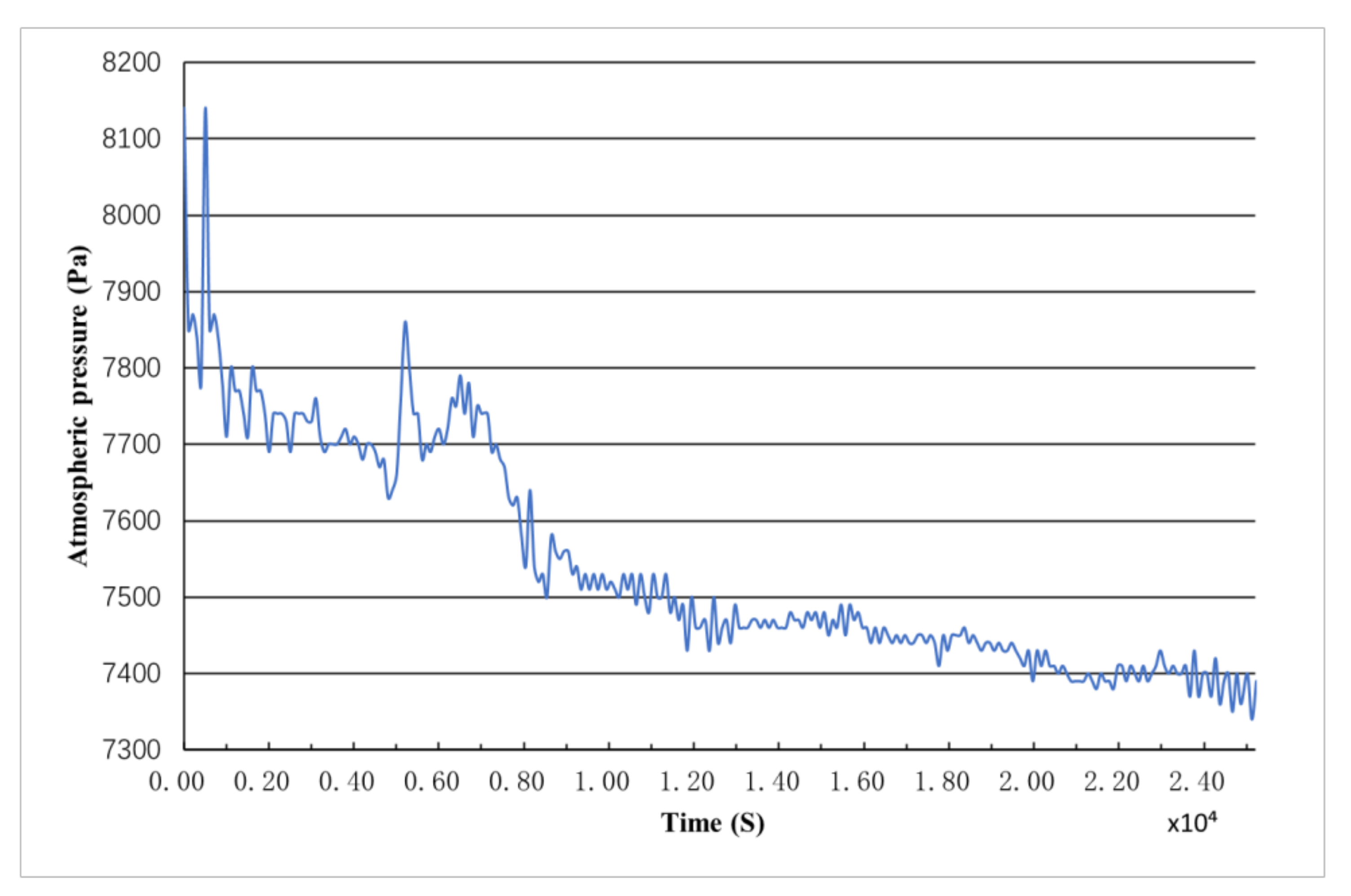
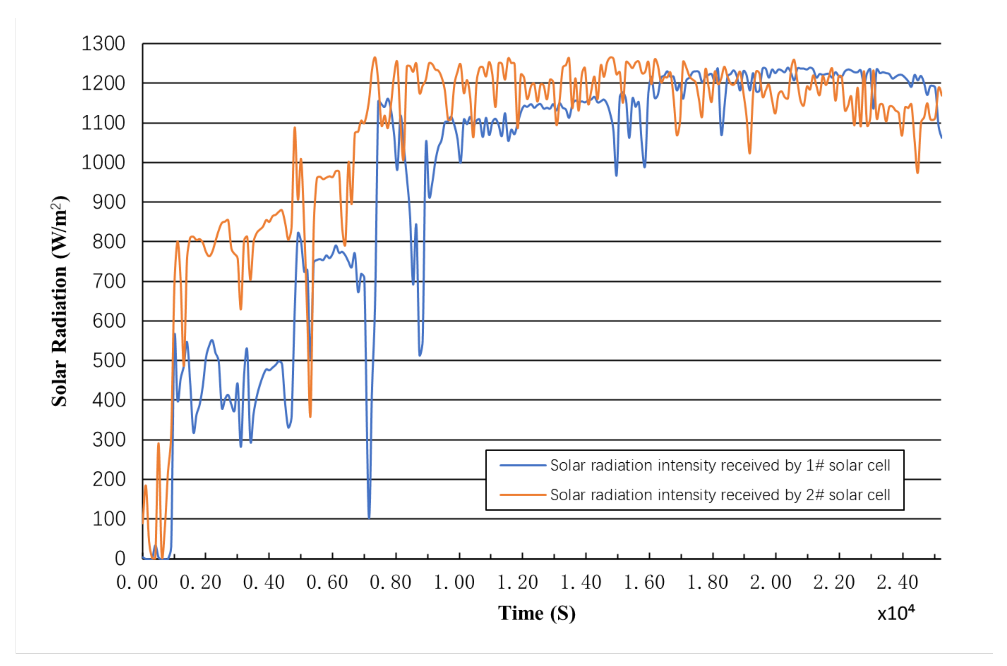
3.1. Overview of the Flight Test

An airship flight test was conducted on 7th Aug. at an altitude of 19 km. The length of the airship is 70 m, and solar cell modules were placed at the top of the airship shown as Figure 4. Two solar cell modules (#1 and #2, about 1 m² each) were tested on board for verification experiments. The solar cell modules are a 10% efficiency flexible thin film CIGS module produced by Ascent Solar company of America.

Table 1. Table of sensors’ parameter and accuracy.

	Type	Measuring Range	Accuracy
Solar radiometer	PMA1144	0–1400 W/m2	0.1 W/m2
Temperature senser	PT100	−100–100 °C	0.35 °C
Barometer	HPA200	0–1213 hPa	0.1 hPa

shows the sensors’ parameter and accuracy.

During the flight test, the airship maintained a cruising altitude. Figure 5, Figure 6, Figure 7 and Figure 8 show the flight velocity of the airship, atmospheric pressure, atmospheric temperature, the solar radiation intensity received by the two modules, and the operating temperature of the modules. Data was gathered in 1 s intervals over a period of approximately 7 h. The 7 h measured data is divided into a training set and a testing set, and the length of the training set is 30 min.

3.2. BPNN Model of Solar Cell Temperature and Simulation Model of Solar Cell Temperature

Based on the same training set samples and testing set samples, the back propagation neural network (BPNN) method is used for prediction [25]. The input layer nodes are atmospheric pressure, solar radiation intensity, flight speed, and ambient temperature. The output layer is the operating temperature of the solar cell modules. The transfer function of the output layer is excited by the logsig function.

The simulation model for operating temperature of solar cell modules on stratospheric airship was established by COMSOL Multiphysics of COMSOL, Inc., Columbus, MA, USA. The solar cell operating temperature data during the entire 7-h flight is obtained through calculation and compared with data predicted by the PSO-SVM model. The simulation parameters are shown as

Table 2. Table of simulation parameters.

Parameter	Value
Length/m	70
Diameter/m	20
Flight date	Aug 21st
Latitude	41°N
Cruising altitude/km	18–19
Types of solar cell modules	CIGS
Temperature coefficient of solar cell modules	−0.4%
Solar cell module area/m2	1
Efficiency of solar cell modules	10%

.

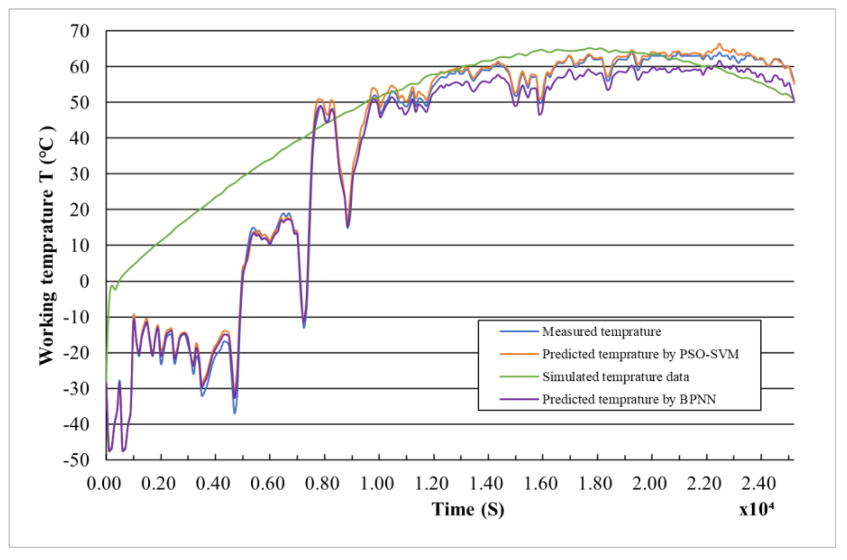
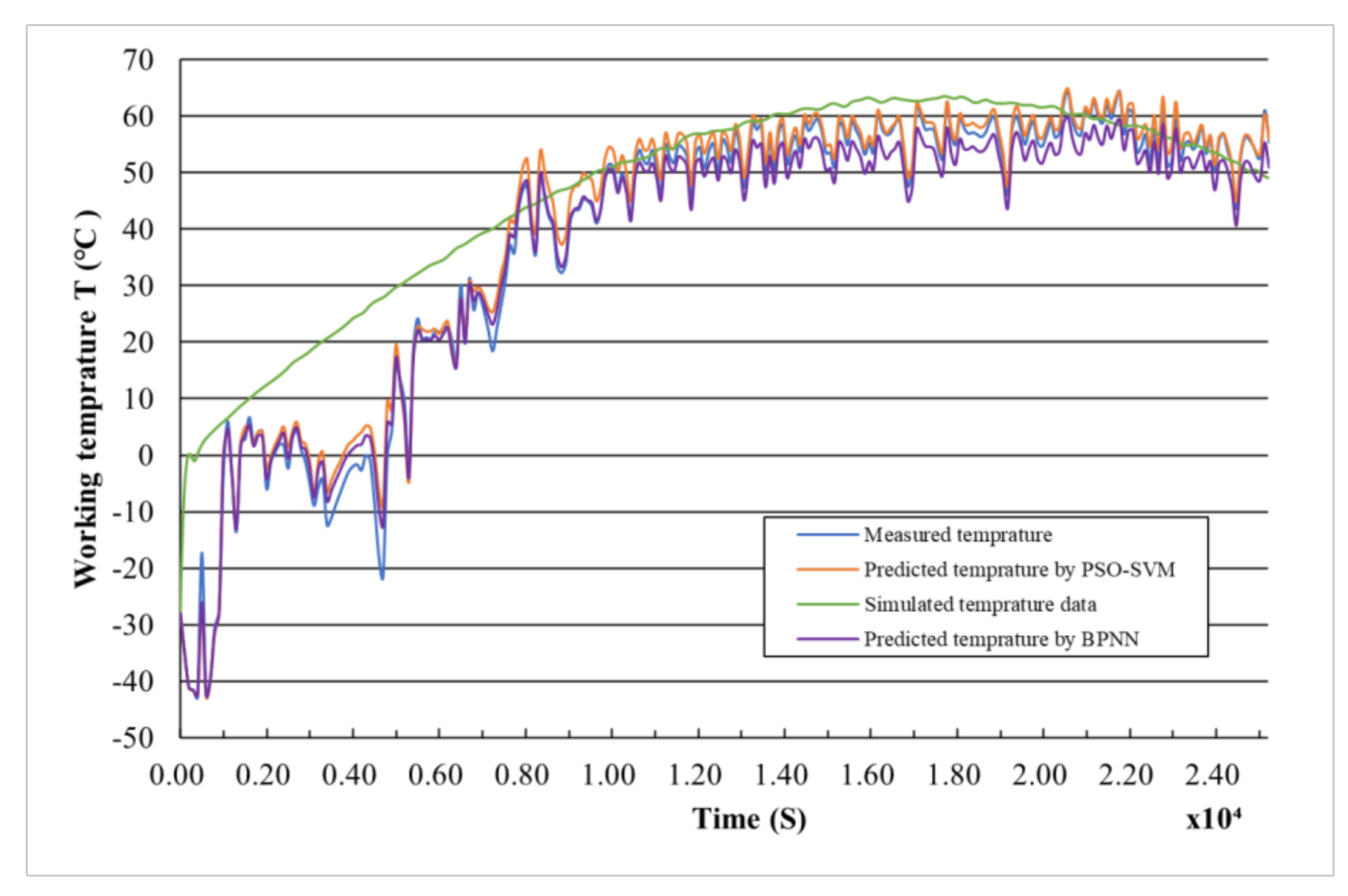
3.3. Comparison between the Measured, Predicted and Simulated Temperature for Solar Cell Module #1

The PSO-SVM calculation model was used to predict the temperature of solar cell module #1. The calculated optimal model parameters are ε = 0.0092, C = 39.4990, and σ = 13.1068. The results were compared with the BPNN model results, the simulated and measured temperature, as shown in Figure 9. The measured temperature (blue curve), predicted temperature by PSO-SVM (orange curve), simulated temperature (green curve) and predicted temperature by BPNN (purple curve) of solar cell module #1 are consistent. The evaluation metrics used were Mean Absolute Error (MAE), Root Mean Square Error (RMSE) and Mean Absolute Percentage Error (MAPE) to comparing the predicted and simulated temperatures’ accuracy shown as

Table 3. Error analysis of the predicted and simulated temperature for solar cell module #1.

	MAE	RMSE	MAPE
The predicted temperature by PSO-SVM	1.4168 °C	0.9869 °C	1.9055%
The predicted temperature by BPNN	2.4679	2.8377	2.7051%
The simulated temperature	12.6907 °C	19.6455 °C	12.8538%

.

According to RMSE of the PSO-SVM model and simulated temperature, the output power of #1 solar cell module errors is 0.3947% and 7.8582%.

3.4. Comparison between the Measured, Predicted and Simulated Temperature for Solar Cell Module #2

The PSO-SVM calculation model was used to predict the temperature of solar cell module #2. The calculated optimal model parameters are ε = 0.0987, C = 39.4319, and σ = 11.1057. The results were compared with the simulated and measured temperature, as shown in Figure 10. The measured (blue curve), predicted by PSO-SVM (orange curve), simulated (green curve) and predicted by BPNN (purple curve) temperature of solar cell module #2 are consistent. The evaluation metrics used were Mean Absolute Error (MAE), Mean Squared Error (MSE), Root Mean Square Error (RMSE) and Mean Absolute Percentage Error (MAPE) to comparing the predicted and simulated temperatures’ accuracy shown as

Table 4. Error analysis of the predicted and simulated temperature for solar cell module #2.

	MAE	RMSE	MAPE
The predicted temperature by PSO-SVM	1.1464 °C	0.5033 °C	1.4133%
The predicted temperature by BPNN	2.4342 °C	2.8297 °C	4.2665%
The simulated temperature	9.2572 °C	13.5102 °C	10.7011%

.

According to RMSE of the PSO-SVM model and simulated temperature, the output power of #2 solar cell module errors is 0.2013% and 5.4041%.

3.5. Summary

The results compared in Section 3.3 and Section 3.4 show that the PSO-SVM temperature prediction model for the solar cell modules of the stratospheric airship established in this article has extremely high prediction accuracy. The prediction model does not depend on the type of airship and the physical characteristics of the solar cell components. It can predict the operating temperature of the cell components through the airship speed, atmospheric pressure, atmospheric temperature and solar radiation intensity. For different types of airships or solar cell modules, using this model to train model parameters through actual measurement data can achieve accurate prediction of the solar cells’ operating temperature. As shown in the calculation example, using the predicting model to predict the temperature of solar cell modules can obtain accurate predicted temperatures.

4. Conclusions

In this study, a particle swarm optimization algorithm-based support vector machine (PSO-SVM) model was used to calculate the operating temperature of solar cell modules on stratospheric airships. The MAPE of predicted data is 1.9055% and 1.4133%, respectively, which is less than the MAPE calculated by BPNN method and much less than the MAPE of simulated data. According to this model, the solar cell modules temperature is related to the atmospheric pressure, solar radiation intensity, airship flight speed, and ambient temperature. Furthermore, the model can be applied to all the types of airship and different physical characteristics of the solar cell components. The accurate prediction of the solar cell modules’ operating temperature can be used to calculate the output power of the solar cell array accurately, and guides the design and energy balance analysis of the PV system of the stratospheric airship.

References

1. Colozza, A.; Dolce, J. Initial Feasibility Assessment of a High Altitude Long Endurance Airship; NASA/CR-2003-212724; NTRS—NASA Technical Reports Server: Brook Park, OH, USA, 2003. [Google Scholar]
2. Revankar, S.; Kota, R. Simulation of solar regenerative fuel cell power system for high altitude airship engineering. Int. J. Adv. Eng. Appl. 2013, 6, 52–64. [Google Scholar]
3. Yu, D.; Lv, X. Configurations analysis for high-altitude/long-endurance airships. Aircr. Eng. Aerosp. Technol. 2010, 82, 48–59. [Google Scholar] [CrossRef]
4. Knaupp, W.; Mundschau, E. Solar electric energy supply at high altitude. Aerosp. Sci. Technol. 2004, 8, 245–254. [Google Scholar] [CrossRef]
5. Liu, J.; Wang, Q.-B.; Zhao, H.-T.; Chen, J.-A.; Qiu, Y.; Duan, D.-P. Optimization design of the stratospheric airship’s power system based on the methodology of orthogonal experiment. J. Zhejiang Univ. Sci. A 2013, 14, 38–46. [Google Scholar] [CrossRef] [Green Version]
6. Soto, W.D.; Klein, S.A.; Beckman, W.A. Improvement and validation of a model for photovoltaic array performance. Sol. Energy 2006, 80, 78–88. [Google Scholar] [CrossRef]
7. Wu, J.; Fang, X.; Wang, Z.; Hou, Z.; Ma, Z.; Zhang, H.; Dai, Q.; Xu, Y. Thermal modeling of stratospheric airships. Prog. Aerosp. Sci. 2015, 75, 26–37. [Google Scholar] [CrossRef]
8. Ju, X.; Vossier, A.; Wang, Z.; Dollet, A.; Flamant, G. An improved temperature estimation method for solar cells operating at high concentrations. Sol. Energy 2013, 93, 80–89. [Google Scholar] [CrossRef]
9. Yao, W.; Lu, X.; Wang, C.; Ma, R. A heat transient model for the thermal behavior prediction of stratospheric airships. Appl. Therm. Eng. 2014, 70, 380–387. [Google Scholar] [CrossRef]
10. Liu, T.T.; Ma, Z.Y.; Yang, X.X.; Zhang, J.S. Influence of Solar Cells on Thermal Characteristics of Stratospheric Airship. J. Astronaut. 2018, 39, 35. [Google Scholar]
11. Colozza, A. Convective Array Cooling for a Solar Powered Aircraft: NASA/CR-2003-212084; NASA: Washington, DC, USA, 2003. [Google Scholar]
12. Li, J.; Lv, M.; Tan, D.; Zhu, W.; Sun, K.; Zhang, Y. Output performance analyses of solar array on stratospheric airship with thermal effect. Appl. Therm. Eng. 2016, 104, 743–750. [Google Scholar] [CrossRef]
13. Li, J.; Lv, M.; Sun, K.; Zhu, W. Thermal insulation performance of lightweight substrate for solar array on stratospheric airships. Appl. Therm. Eng. 2016, 107, 1158–1165. [Google Scholar] [CrossRef]
14. Lv, M.; Li, J.; Du, H.; Zhu, W.; Meng, J. Solar array layout optimization for stratospheric airships using numerical method. Energy Convers. Manag. 2016, 135, 160–169. [Google Scholar] [CrossRef]
15. Kea G, A. Solar panel area estimation and optimization for geostation ary stratospheric airships. Am. Inst. Aeronaut. Astronaut. 2011, 6974, 1–13. [Google Scholar]
16. Li, X.; Fang, X.; Dai, Q. Research on thermal characteristics of photovoltaic array of stratospheric airship. J. Aircr. 2011, 48, 1380–1386. [Google Scholar] [CrossRef]
17. Wang, H.; Song, B.; Zuo, L. Effect of High-altitude airship’s attitude on performance of its energy system. J. Aircr. 2007, 44, 2077–2080. [Google Scholar] [CrossRef]
18. Sun, K.; Yang, Q.; Yang, Y.; Wang, S.; Xu, J.; Liu, Q.; Xie, Y.; Lou, P. Thermal Characteristics of Multilayer Insulation Materials for Flexible Thin-Film Solar Cell Array of Stratospheric Airship. Adv. Mater. Sci. Eng. 2014, 2014, 1–8. [Google Scholar] [CrossRef] [Green Version]
19. Rahim, N.A.; Chaniago, K.; Selvaraj, J. Single-Phase Seven-Level Grid-Connected Inverter for Photovoltaic System. IEEE Trans. Ind. Electron. 2011, 58, 2435–2443. [Google Scholar] [CrossRef]
20. Yona, A.; Senjyu, T.; Funabashi, T. Application of Recurrent Neural Network to Short-Term-Ahead Generating Power Forecasting for Photovoltaic System. In Proceedings of the Power Engineering Society General Meeting, Tampa, FL, USA, 24–28 June 2007; IEEE: Piscataway, NJ, USA, 2007. [Google Scholar]
21. Rai, A.K.; Kaushika, N.D.; Singh, B.; Agarwal, N. Simulation model of ANN based maximum power point tracking controller for solar PV system. Sol. Energy Mater. Sol. Cells 2011, 95, 773–778. [Google Scholar] [CrossRef]
22. Ishaque, K.; Salam, Z.; Amjad, M.; Mekhilef, S. An Improved Particle Swarm Optimization (PSO) based MPPT for PV with Reduced Steady State Oscillation. IEEE Trans. Power Electron. 2012, 27, 3627–33638. [Google Scholar] [CrossRef]
23. Ma, G.; Lv, M.; Li, J. Numerical Model of Thermal Performance for Solar Array on Stratospheric Airship. Sci. Technol. Eng. 2017, 17, 115–154. (In Chinese) [Google Scholar]
24. Wang, W.; Men, C. Support Vector Machine Modeling and Its Application; Science Press: Beijing, China, 2014; p. 211. (In Chinese) [Google Scholar]
25. Ceylan, İ.; Erkaymaz, O.; Gedik, E.; Gürel, A.E. The prediction of photovoltaic module temperature with artificial neural networks. Case Stud. Therm. Eng. 2014, 3, 11–20. [Google Scholar] [CrossRef] [Green Version]
Figure 1. Thermal model for a solar cell array on an airship.
Energies 14 01228 g001
Figure 2. Flowchart of optimization solving scheme.
Energies 14 01228 g002
Figure 3. Flow chart for calculating the operating temperature of a solar cell with the PSO-SVM model.
Energies 14 01228 g003
Figure 4. Diagram of solar cell modules layout.
Energies 14 01228 g004
Figure 5. Measured airship flight velocity during a flight test.
Energies 14 01228 g005
Figure 6. Measured atmospheric pressure during a flight test.
Energies 14 01228 g006
Figure 7. Measured solar radiation intensity on two solar cell modules during a flight test.
Energies 14 01228 g007
Figure 8. Measured data of two solar cell module’s operating temperature during flight test.
Energies 14 01228 g008
Figure 9. Comparison between the measured, predicted and simulated operating temperature of solar cell module #1.
Energies 14 01228 g009
Figure 10. Comparison between the measured, predicted and simulated operating temperature of solar cell module #2.
Energies 14 01228 g010